Overview of Bayesian sequential Monte Carlo methods for group and extended object tracking

Contents lists available atScienceDirect

Digital Signal Processing

www.elsevier.com/locate/dsp

Overview of Bayesian sequential Monte Carlo methods for group and

extended object tracking

Lyudmila Mihaylova

a,

∗

, Avishy Y. Carmi

b

, François Septier

c

, Amadou Gning

d

,

Sze Kim Pang

e

, Simon Godsill

f

a_{University of Sheffield, Department of Automatic Control and Systems Engineering, Mappin Street, Sheffield S1 3JD, United Kingdom} b_{Ben-Gurion University of the Negev, Department of Mechanical Engineering, Beer-Sheba 8410501, Israel}

c_{Institut Mines-Télécom / Télécom Lille 1 / LAGIS UMR CNRS 8219, Cité Scientifique, Rue Guglielmo Marconi, BP 20145, 59653 Villeneuve d’Ascq Cedex, France} d_{University College London, Computer Science Department, United Kingdom}

e_{DSO, Singapore}

f_{University of Cambridge, Department of Engineering, United Kingdom}

a r t i c l e

i n f o

a b s t r a c t

Article history:

Available online 4 December 2013

Keywords:

Sequential Monte Carlo methods Group and extended object tracking Markov chain Monte Carlo methods Nonlinear filtering

Metropolis Hastings Reasoning over time

This work presents the current state-of-the-art in techniques for tracking a number of objects moving in a coordinated and interacting fashion. Groups are structured objects characterized with particular motion patterns. The group can be comprised of a small number of interacting objects (e.g. pedestrians, sport players, convoy of cars) or of hundreds or thousands of components such as crowds of people. The group object tracking is closely linked with extended object tracking but at the same time has particular features which differentiate it from extended objects. Extended objects, such as in maritime surveillance, are characterized by their kinematic states and their size or volume. Both group and extended objects give rise to a varying number of measurements and require trajectory maintenance. An emphasis is given here to sequential Monte Carlo (SMC) methods and their variants. Methods for small groups and for large groups are presented, including Markov Chain Monte Carlo (MCMC) methods, the random matrices approach and Random Finite Set Statistics methods. Efficient real-time implementations are discussed which are able to deal with the high dimensionality and provide high accuracy. Future trends and avenues are traced.

©2013 The Authors. Published by Elsevier Inc.

1. Motivation: Why is group and extended object tracking important? Differences and similarities

In recent years there has been an increasing interest in track-ing a number of objects movtrack-ing in a coordinated and interacttrack-ing fashion. There are many fields in which such situations are fre-quently encountered: video surveillance, sport events, biomedicine, neuroscience, meteorology, situation awareness and search rescue operations, to mention but a few. Although individual objects in the group can exhibit independent movement at a certain level, overall the group moves as one whole, synchronously with respect to the individual entities and avoiding collisions.

Terminology.Groups are structured objects, formations of enti-ties moving in a coordinated manner, whose number varies over time because targets can enter a scene, or disappear at random

*

Corresponding author.

E-mail addresses:l.s.mihaylova@sheffield.ac.uk(L. Mihaylova),

[email protected](A.Y. Carmi),[email protected](F. Septier), [email protected](A. Gning),[email protected](S.K. Pang),[email protected] (S. Godsill).

times. The groups can split, merge, can be relatively near to each other or move independently of each other. What is typical for group formations is that they maintain certain patterns of motion. Some typical examples are: formations of aircrafts and ships, re-spectively, for air traffic control, sea, harbor or land surveillance [45,124], flocks of bird migration trajectories for ecological pur-poses, tracking groups of cells [38,107,149,127] (for in vitro pur-poses, stem cells, cardiovascular treatment and other medical diag-nostics), a group of robots (for industrial tasks), a group of football players [152] in sport videos, convoys of vehicles and groups of pedestrians for traffic management[3]. Within this broad range of problems, one can distinguish two main classes: (1) tracking of multiple groups with only a few components per group, which is calledsmall groups tracking, and (2) groups with a relatively large number of constituents whose individual members cannot be eas-ily distinguished, termedlarge groups. Large groups are also often referred as tocrowdsorclusters.

A related but distinct is the problem of tracking extended ob-jects, such as a cyclist and maritime vessels [5]. Extended objects cannot be considered as points but instead have a spatial extent characterizing their size or volume[74]. They are usually modeled

http://dx.doi.org/10.1016/j.dsp.2013.11.006

1051-2004©2013 The Authors. Published by Elsevier Inc.

Open access under CC BY-NC-ND license.

[image:2.612.77.554.56.279.2]

Fig. 1.Taxonomy of sequential Monte Carlo methods for tracking a small number of groups with only a few objects.

with simple geometrical shapes which are typically circles[111], ellipses[117], rectangles[10,11,51,55,56], closed contours or arbi-trary shapes such as star-convex contours[9]. Other examples are tracking a cloud [69,122] of radio-active materials and a human face or hand in video[21]. Human body limb tracking is also often referred to extended target tracking.

Challenges and differences. The challenges in solving the task for groups with a small number of components differ from those of groups with a large number of components. In small groups it is possible to model the interactions and interrelationships between the components within a group. The difficulties with groups of hundreds or thousands of objects (such as pedestrians and riots in video surveillance and radar based tracking of hundreds of aircraft) are mainly due to two reasons: (1) the individual objects cannot be distinguished/identified within the group, (2) the information and features extracted by the sensors are not sufficient to track those objects. Hence, one considers the aggregated motion of the whole group. In small groups one can estimate the states of each par-ticular object and parameters characterizing the size or volume of the group. In large groups by contrast, one typically considers the group as a geometric shape and its centre coordinates.

Similarities. Both groups of objects and extended objects give rise to a large, varying number of measurements and require a flexible framework able to deal with all these challenges. Although the methods for solving these two kinds of problems vary, there is a common approach in which both extended and large group of targets are seen as the same problem. The large group or extended object is surrounded with a shape (e.g. a circle) and the center and extent of this shape are sequentially computed based on the incoming data. Consequently, in this paper, the choice is made to classify the existing works in the literature into methods dealing with small groups and method dealing with large groups and for extended objects.

This classification of extended/group objects is according to whether: (1) the group/extended object is rigid and unchanging in shape/size, (2) whether individual entities can be tracked dy-namically and interact with one another.

Examples of non-rigid extended objects are radioactive clouds. They can be spawn and also disappear. The group tracking and non-rigid extended object tracking lead to dynamic state and vary-ing parameter estimation. Rigid extended targets such as

sub-marines, ships, have fixed shapes and fixed size. This leads to dynamic state and static parameter estimation.

1.1. Objectives

The aim of this paper is to expose the reader to the various aspects of the problems of group and extended object tracking, un-derlying difficulties, and the key factors facilitating their solution in the context of Bayesian estimation. An overview of the state-of-the-art concepts and methodologies underlying contemporary Monte Carlo-based group and extended object tracking schemes is provided. The taxonomy of methods is given in Section 1.2and background knowledge in Section2. Methodologies for small group tracking are described in Section 3 and for large groups and ex-tended objects in Section 4. The high dimensionality of the prob-lem and the need of real time impprob-lementation calls for efficient algorithmic implementations, in a distributed and parallelized way, which are discussed in Section5. Future avenues are summarized in Section6.

1.2. Taxonomy of methods for multiple groups and extended object tracking

Over the past decade various methods have been developed for group and extended object tracking. These can be divided into two broad classes depending on the underlying complexities:

1. Methods for a relatively small number of groups, with a small number of group components[51,109,76,6].

2. Methods for groups comprised of hundreds or thousands of objects (normally referred to as cluster/extended object/crowd tracking): track before detect methods for extended ob-jects [18,17], Poisson likelihood approaches [48,49,120,22], groups’ extent parameter estimation and random matrix techniques [5,8,75,74,46], parametric level curves [69,122], and random finite sets [94,143,136,137,86,91], including the Bernouli random finite set filters[116,113].

Figs. 1 and 2 present the taxonomy of methods for tracking small groups and respectively large groups/extended objects. De-tails are given in the next sections.

[image:3.612.51.564.55.260.2]

Fig. 2.Taxonomy of sequential Monte Carlo methods for tracking large groups and extended objects.

process formulations for properly assigning measurements to their originating targets. As part of this, smart procedures are used to eliminate non-probable association hypotheses. Other SMC schemes adopt various approaches for dealing with the high di-mensionality problem[121,77].

An extension of the SMC technique to a varying number of tar-gets is introduced in[141]and[73]. In[73,109]sequential Markov Chain Monte Carlo (MCMC) techniques are developed for track-ing varytrack-ing numbers of interacttrack-ing objects. The MCMC approach has advantages over the conventional particle filter (PF) due to its efficient sampling mechanism [24,22,109]. Interacting popula-tion MCMC algorithms are presented in[16,15,14]. The approach proposed in [36] represents an extension of the MCMC method proposed in[73]. However, in[36]measurement clustering is com-bined with nonparametric prior information and the variational Bayes approach.

1.2.1. Methods for small groups

The methods for tracking small groups can be further divided into: (1) methods that take into account the interactions between group components and (2) methods that ignore such interactions. The latter class of methods are the standard Bayesian techniques that track each object separately (e.g., generic particle filters, Ex-tended Kalman filters, Unscented Kalman Filters, Multiple Hypoth-esis Tracking (MHT) filters [6] and others). These methods have been extensively studied in the literature[114,89].

The former class of methods which consider object’ interactions is much more compelling (see e.g.[71,72,7,73]). Although it has received attention in recent years, there is still a wealth of chal-lenges most of which concern the group structure evolution and transitions[89,55].

[image:3.612.317.557.286.496.2]

The predominant strategy consists in incorporating local inter-action rules into the object state dynamics. Normally, individual objects are labeled[109] and tracked along with the group struc-ture[51]. For a small number of objects, one obtains only a few likely group structures. The object states are updated at every time step using models for appearance(birth) of an object, or dis-appearance (death) of an object and spawning objects [89,29,108, 94,93]. Analogously, the group structure is updated taking into account only a few admissible transitions which are determined from physical constraints such as groups’ spatial extent and prox-imity. Interactions at the group level are subject to transitions in addition to the aforementioned ones. Thus, apart from birth and

Fig. 3.Dynamics of a small group structure over time. Splitting takes place from timet1 tot2, resulting with a new group (white). From timet2, the white group

splits again and merges with the red and blue groups, giving rise to entirely new (green and grey) configurations. The arrows represent the entities movement direc-tion. (For interpretation of the references to color in this figure legend, the reader is referred to the web version of this article.)

disappearance, two additional moves that are commonly attributed to groups aresplittingandmerging.

Alternatively, group structure dynamics can be modeled by means of graph-theoretic approaches and evolving networks[51]. In this approach, group components take the role of vertices in a graph where edges embody interrelations among objects. As the group evolves over time, the graph is adapted to reflect the in-stantaneous structure. This essentially involves removing or adding nodes and updating edges accordingly. Markov random fields can be used in a similar fashion for modeling group interactions [71, 72,7,73]. Other works use the multi-goal social force model[100, 110]for pedestrian tracking which extends the social force model proposed in[62]or macroscopic models[28].

time step t1 there are two groups: group 1 with three

compo-nents (the upper group, indicated in red) and group 2, with three components (the lower group, indicated in blue). The empty cir-cles correspond to noisy measurements (e.g. clutter1_{). Splitting and} merging is demonstrated in the 2nd and 3rd time-steps, respec-tively. For clarity, objects’ interrelations are mostly omitted in this depiction. They are, nevertheless, suggested for the last time-step in the right-hand-side ellipses.

1.2.2. Methods for large groups and extended objects

When the number of entities becomes excessively large it is impractical to track them all individually. Thus, instead of track-ing separate components, large group techniques identify and track concentrations, e.g. the center of the group and its extent parame-ter. In this respect groups and extended object tracking are similar problems. The entities forming the concentrations may be objects, measurements or features. This strategy is applied in practice by utilizing extent variables which represent the spatial shape and dynamics of a group. In typical scenarios, groups are characterized by the location and velocity of the group center, their shape and shape deformation[9].

Another promising approach for modeling large groups is based on the social force model[101,2].

For large groups (and extended objects), the group density and shape are closely related. The posterior pdf of the joint state and extent parameter vector can, for example, be considered as a mix-ture of Gaussians [22]. This is primarily due to the convenient parametric representation which involves the first two statistical moments of the Gaussians, but other representations are possible. Here, the mean and covariance of the Gaussian mixture are, re-spectively, the center and shape of the group or extended object. Normally, the extent parameters are considered as both random and dynamic, and as such are governed by appropriate transition kernels. These approaches are capable of simulating complex dy-namically evolving shape boundaries, and even compete with so-phisticated contour tracking methodologies (see for example[69, 122]).

The measurement origin uncertainty in group and extended ob-jects can be dealt with in an efficient way [48,49,120,22] if the numbers of received target and clutter measurements are consid-ered Poisson distributed (implying that several measurements may originate from each target).

A different, albeit related, modeling approach is considered in [5,8,75,74,46]where the group extent represents a parameter, es-timated as part of an augmented state vector, jointly with the position coordinates of the group center. Except for [5], all other works in this group employ either Kalman filtering techniques[6] or random finite set approaches[89]. In general, the extent is con-sidered as a random process and hence is normally assigned a respective prior (e.g., Wishart distribution[75,74,46]) and a transi-tion kernel.

The random finite set approach is a powerful tool that has been widely used in recent years[89]. Random finite sets are mathemat-ical objects that can elegantly capture the subtleties involved in multiple object tracking and data fusion. It was not until recently that these methods have been employed for group and extended object tracking. The works [94,143,136,137] demonstrate the vi-ability of the well-known Probvi-ability Hypothesis Density (PHD) filter in solving group tracking problems. These approaches are dis-cussed extensively in the methodological part of this paper.

Fluid dynamic models have also been shown to capture well aggregated vehicular traffic phenomena, in combination with SMC

1 _{In radar applications clutter signifies signal reflected from the environment,}

in-stead of from the objects of interest.

methods[103], for the purposes of freeway traffic tracking. A large body of work is devoted for modeling pedestrians flows in open and enclosed regions, e.g.[67,81,153]and weather forecasts[138]. In what follows, we present the generic SMC framework fol-lowed by more sophisticated approaches.

2. Background knowledge

Consider the discrete-time nonlinear non-Gaussian motion model

xk

=

f

(

xk−1

,

vk−1

),

(1)

zk

=

h(xk

,

nk

),

(2)

where xk is the system state vector which has to be estimated in time k

=

1

,

2

, . . .

; zk represents the measurement obtained at timek; f

(.)

andh

(.)

are nonlinear system and measurement func-tions, respectively;vkandnkare mutually independent noise vec-tors, respectively, the system noise and the measurement noise. The state vectorxk characterizes the objects of interest and jointly with f

(.)

describe the motion interactions of the objects.

2.1. Generic particle filters

The aim of SMC methods, known also as particle filters [54, 41,43,61,119,39,27] is to represent with “particles” the posterior state probability density function given the sensor measurements, p

(

xk

|

Z0:k

)

, where Z0:k

= {

z0

, . . . ,

zk

}

is the observation history up to time k. Two major stages can be distinguished: prediction and update. During prediction, each particle (point mass representa-tion of the probability density) is modified according to the state model, including the addition of random noise in order to simulate the effect of the noise on the state. In the measurement update stage, each particle’s weight is re-evaluated based on the new data. Hence, during the prediction step the “cloud of particles” is usu-ally spread/expanded due to the system noise, whereas the mea-surement update step contributes particles to concentrate around the system states. Hence, the weighted particles

{

xi_k

,

wi_k

}

_iN₌₁ are propagated through the motion model(1)and updated next upon the measurement arrival, based on the measurement equation(2). An inherent problem with particle filters (PFs) is degeneracy, the case when only one particle has a significant weight and the oth-ers are close to zero. The sampling importance resampling (SIR) SMC avoids the degeneracy by adding an extra resampling step. An estimate of the measure of degeneracy at time k is given as Neff

=

1

/

N

=1

(

wik

)

2 _{[41]. If the number N}

eff of efficient particles is below a user defined threshold Nthreshold, the resampling pro-cedure introduces variety in the particles, and can help to avoid degeneracy by eliminating particles with small weights and repli-cating particles with larger weights.

The algorithm of the generic PF is summarized inTable 1. The estimate of the variable of interest is obtained by a weighted sum of particles.

Table 1

Generic particle filter algorithm.

[{xi

k,wki}Ni=1] =PF[{xik−1,wik−1}Ni=1,zk]

fori=1:N(for each particle)do

– Drawxiksamples based on the motion model(1)

– Determine the weight update factors based on the likelihood function calculated from the measurement model(2).

– Normalize weights,wi k=w

i k/

N i=1wik

ifNeff_<Nthreshold_then – Resample particles. end

– Calculate the expected state:E[xk|zk] =Ni=1wikxki.

Different proposal distributions have been used in the SMC framework – the most common transition prior or more advanced priors using the latest measurements, MCMC steps and others such as conjugate priors (e.g. inverse Wishart distribution[75,74,46]).

Section2.2considers Markov Chain Monte Carlo (MCMC) meth-ods.

2.2. Sequential Bayesian inference using Markov Chain Monte Carlo methods

The Bayesian framework provides efficient ways of computing the desired posterior distribution. Unfortunately, in many appli-cations, this distribution is analytically intractable. SMC methods such as particle filtering can be used to carry out the infer-ence by sequentially approximating this posterior distribution as in[51]. MCMC methods are generally more effective than PFs in high-dimensional spaces. Their traditional formulation, however, allows sampling from probability distributions in a non-sequential fashion. Recently, advanced sequential MCMC schemes were pro-posed in [12,73,109,123]. These approaches are distinct from the Resample-Move scheme[50] where the MCMC algorithm is used to rejuvenate degenerate samples following importance sampling resampling. These methods[109,73,12]use neither resampling nor importance sampling.

In attempting to circumvent the degeneracy problems that can possibly arise in PFs in high dimensions (e.g. with more than 20 states), the Markov Chain Monte Carlo (MCMC) framework[22,71, 72,7,73] is investigated and is shown to be effective. The MCMC technique arise first in statistical physics[83,118]. The underlying principle consists in constructing a Markov chain whose long-term equilibrium is close to a desired probability distribution. The addi-tion of the MCMC steps affords moving the “cloud of particles” into more likely regions which improves significantly the performance of the obtained sequential filters. The MCMC step also allows sim-ulation of complicated systems that are difficult to deal with di-rectly, including interactions between group components. Another advantage is that the MCMC step leads to flexibility and one can sample only a part of the state conditional upon the rest, thus fa-cilitating efficient samples.

There are many different ways to perform the MCMC steps. One of the most common MCMC algorithms is the Metropolis–Hastings (MH) move step, where first a likelihood ratio test is calculated (based on particles from two subsequent iterations) and the par-ticle is selected if the likelihood exceeds a certain threshold. For small groups tracking the MH step was proposed in [109] and in[51] and shows efficient results. The method from [109] aims at sequentially approximating the following joint posterior distri-bution

p(Xk

,

Xk−1

|

Z0:k

)

∝

p(Zk

|

Xk

)p(

Xk

|

Xk−1

)p(

Xk−1

|

Z0:k−1

),

(3)

where the state vector Xk2 comprises the objects’ instantaneous position, velocity and extent parameters at timek.

Since the closed form expression of the distribution p

(

Xk−1|

Z0:k−1

)

is generally unknown, the proposed scheme approximates

it by usingNpunweighted particles

p(Xk−1

|

Z0:k−1

)

≈

1 N

N

j=1

δ

Xk−1

−

X_k(₋j)₁

,

(4)

where

δ(.)

is the Dirac delta function and

(

j

)

is the particle index. Then, by applying this particle approximation to(3), an appropri-ate MCMC scheme can draw samples from the joint posterior pdf p

(

Xk

,

Xk−1

|

Z0:k

)

. The converged MCMC outputs are then extracted

2 _{Note that we will denote the state vector in the reminder of the paper with a}

[image:5.612.311.562.77.263.2]

capital letter to emphasize that it contains both states and extent parameters.

Table 2

Sequential MCMC algorithm.

Initialize particle set{X(₋j1)}jN=1fork=1, . . . ,Tdo

form=1, . . . ,NMCMCdo

Joint Draw

– Propose{X∗_k,X∗_k−1} ∼q1(Xk,Xk−1|Xmk−1,X m−1

k−1)

– Compute the MH acceptance probability

ρ1=min

1, p(X

∗ k,X∗k−1|Z0:k)

q1(X∗k,Xk−∗1|Xm−k 1,Xm−k−11)

q1(Xm−k 1,Xm−

1

k−1|X∗k,X∗k−1)

p(Xm−1

k ,Xm−k−11|Z0:k)

– Accept{Xm

k,Xmk−1} = {Xk∗,X∗k−1}with probabilityρ1 Block Refinement

– Randomly divideXkintoPblocks{Ωp}pP=1

forp=1, . . . ,Pdo

– Propose{Xk∗,Ωp} ∼q(Xk,Ωp|X

m k,\Ωp,X

m k−1)

– Compute the MH acceptance probability

ρp=min

1,p(X

∗ k,Ωp|X

m k,\Ωp,X

m k−1,Z0:k)

q(X∗ k,Ωp|X

m k,\Ωp,X

m k−1)

q(Xm k,Ωp|X

m k,\Ωp,X

m k−1)

p(Xm k,Ωp|X

m k,\Ωp,X

m k−1,Z0:k)

– Accept{Xm k,Ωp} = {X

∗

k,Ωp}with probabilityρp

end end end

to give an empirical approximation of the posterior distribution of interest at timek, thus seeding the next filtering step at time k

+

1.

As shown in [109] and in [22], in high dimensional spaces the combination of Metropolis–Hastings with Gibbs sampling gives efficient results and can overcome possible degeneracy problems of PFs. The derived sequential MCMC algorithm has two steps, for drawing samples fromp

(

Xk

,

Xk−1|Z0:k

)

:

1. Make a joint draw for the pair

{

Xk

,

Xk−1}using a Metropolis– Hastings step,

2. Divide Xk into P sub-blocks, Xk

= [

Xk,Ω1

, . . . ,

Xk,ΩP

]

. Then

each sub-block can be updated either via a random scan or a deterministic scan using a series of MH-within-Gibbs steps.

The script for the MCMC algorithm is given inTable 2. Other methods such as the particle MCMC methods proposed in[4]have potential but still have not been studied in the light of the group and extended object tracking problems mainly because these algorithms are used to solve off-line problems.

The next section presents methods for tracking small groups.

3. Methods for tracking small groups

Methods for small group tracking are part of surveillance and monitoring systems and are often meant to provide both state esti-mates and knowledge about their interactions and group behavior. We firstly describe the Bayesian formulation of the problem with a discussion on the group structure. Then, biologically inspired in-teraction models capturing interdependencies among objects are presented.

3.1. Bayesian problem formulation

The problem of tracking groups with a small number of com-ponents consists in estimating an augmented state vectorXk con-taining the states of all groups, at discrete timek, with their com-ponents, given a parameter vector Gk characterizing the structure of all groups. At timekwhen a measurement vectorzkis received, the measurement likelihood function p

(

zk

|

Xk

)

can be calculated, and hence the state pdf for each group of objects.

[image:6.612.82.509.56.165.2]

Fig. 4.Boids system and virtual leader local interaction rules. The blue and red arrows represent object velocities and restoring forces, respectively. The position of the virtual leader is illustrated by a yellow circle in each group. (For interpretation of the references to color in this figure legend, the reader is referred to the web version of this article.)

p(Xk

,

Gk

|

Z0:k−1

)

=

p(Gk

|

Xk

,

Z0:k−1

)p(

Xk

|

Z0:k−1

)

=

p(Gk

|

Xk

,

Gk−1

)p(

Xk

|

Xk−1

,

Gk−1

)

×

p(Xk−1

,

Gk−1

|

Z0:k−1

)

dXk−1dGk−1

,

(5)

p(Xk

,

Gk

|

Z0:k

)

=

p(zk

|

Xk

,

Gk

)p(

Xk

,

Gk

|

Z0:k−1

)

p(zk

|

Z0:k−1

)

,

(6)

wherezkandZ0:kdenote the measurement at timekand the mea-surement history up to timek, respectively.

The transition pdf p

(

Gk

|

Xk

,

Gk−1

)

of the group structure can

be calculated in two ways. In [109] a prior transition matrix be-tween the discrete possible group structures while in [51] the group structure model based on graphical network models is used. In this second approach the nodes of the graph correspond to the components of the group. The presence of an edge between two nodes reflects a link between these two objects. Merging, split-ting, spawning and birth of groups are all modeled within the framework of evolving graphs and by taking into account geo-metrical distances between groups and within group components. Prediction is performed by an evolution model for the group/graph structure[51].

Next, the transition pdf p

(

Xk

|

Xk−1

,

Gk−1

)

of the state of all

targets is calculated knowing the previous time target states and group structure. With the assumption of independence between group motions, the pdfp

(

Xk

|

Xk−1

,

Gk−1

)

can be decomposed as

p(Xk

|

Xk−1

,

Gk−1

)

=

g∈Gk−1

p

Xg_k

X

g_k−1

,

(7)

where p

(

X_kg

|

X_kg₋₁

)

is the transition density of the set of targets from theg-th group.

The group structure can be represented in different ways. In [108],Gkrepresents a set of group’s labels for each target. For ex-ample, with five targets,Gk

= [

1 1 2 2 2

]

means that targets 1 and 2 are in group 1 and targets 3, 4 and 5 are in group 2.

The group structure can be represented also as a random graph as shown in [51]. Consider N targets constituting the set of ver-tices

{

v1

, . . . ,

vN

}

. Each vertexviis associated with the target state and with the target state’s corresponding variance. The set of edges linking the set of vertices is denoted byE. The graph structure can then be denoted byG

=

(

{

v1

, . . . ,

vN

}

,

E

)

. One edge, in E, between two nodesviandvjis denoted by

(

vi

,

vj

)

. In order to characterize the presence or absence of a link (edge) between two nodes, the distance between these two considered nodes is calculated, e.g., by the Mahalanobis distance criterion. In the previous example dis-cussed, with the graphical representation, one group structure is:

Gk

=

(

{

v1

,

v2

,

v3

,

v4

,

v5}

,

{

(

v1

,

v2

), (

v3

,

v4

), (

v3

,

v5

)

}

)

and the groups

correspond to the connected components of the graphGk. The Ma-halanobis distance is computed from the estimated positions and from the velocities of the separate objects. This estimated distance is thresholded and a decision is made about the connections. In

this representation a group corresponds to aconnected component of the graph structure. Note that, two nodes are in the same con-nected component if and only if a path between them exists. The Matlab code for the algorithm presented in this section is available on Matlab Central[98].

Algorithms for group birth, death, splitting and merging are proposed in [51] by taking into account geometric distances and velocity distances between the groups and between the separate group components.

The next subsection presents interaction models and results in-spired by biological systems.

3.2. Biologically inspired and social interaction models

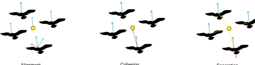
Many of the group object tracking approaches are developed by seeking similarities with emerging behaviors in complex bio-logical systems, such as flocking, swarming, herding and schooling. In such models [63,148,26], local interaction rules maintain coor-dination among individuals. This in turn gives rise to a collective behavior which may be qualitatively different from the superposi-tion of the separate components. A common modeling concepsuperposi-tion, known as Boids, embodies the following set of local interaction rules[112]:separation, alignmentandcohesion. For instance, a flock of birds tends to move in a way to avoid crowding local flockmates and keeps a certain distance between each other, which is an ex-ample ofseparation. The group constituents tend to steer towards the average heading of local flockmates and hence achieves align-ment. Lastly,cohesionsustains a certain amount of coherence of the flock motion as individuals tend to move towards the average po-sition of local flockmates. The flocks of birds usually have a leader. This has inspired the development of the so calledleader–follower models. The leader–follower model describes a behavior in which each member of a group interacts with an aggregative, yet virtual object. In [109], this concept has been conveniently formulated in continuous time through a multivariate stochastic differential equation and then derived in discrete time without approxima-tion errors, owing to the assumed linear and Gaussian form of the model. In particular, two different models are proposed. In the first, the basic group model and the group parameter are repre-sented as a deterministic function of the objects. The second is a group model with a virtual leader. An additional state variable is introduced to characterize the group or bulk parameter. This sec-ond approach is closer in spirit to the bulk velocity model and virtual leader–follower model [89]. Such model provides a more flexible behavior since the virtual leader is no longer a determinis-tic function of the individual object states.Fig. 4gives a graphical illustration of the restoring forces towards the virtual leader for a flock of four birds.

by experiments in sea navigation. A broad range of models for pedestrians and crowds tracking are proposed in[2].

The spatio-temporal structure for theith object in a group, as defined in[109], is given by:

d

˙

xt,i

/dt

=

−

α

[

xt,i

−

vt

] −

γ

1x

˙

t,i

−

β

[˙

xt,i

− ˙

vt

] +

ri

+

dWt,i

/dt

,

(8)

dv

˙

t

/dt

= −

γ

2v

˙

t

+

dLt

/dt.

(9)

Herext,i is the Cartesian position in the xdirection of theith object of the group at continuous time t, with

˙

xt,i is the corre-sponding velocity; vt and v

˙

t represent respectively the Cartesian position and the velocity both in the X direction of the unob-served virtual leader of the group;W_tx_,i andL_tx are two indepen-dent Brownian motion processes, with Wt,i being assumed to be independently generated for each objectiin the group, whereasLt is a noise component common to all members of a group. The pa-rameters

α

and

β

are positive, and reflect the strength of the pull towards the group center. The terms

γ

1

˙

xt,i and

γ

2v

˙

t simply pre-vent the velocities of the object and the virtual leader drifting up to very large values with time. Finally, to avoid colocation or spa-tial collision of group components, an additional repulsive forceri is introduced in(8) when objects become too close. The positive constants

γ

1 and

γ

2 give different weights of the two terms in(8)

and(9), respectively. The spatio-temporal model(8)and(9)can be used to define the prior transition of the objects in(6).

The likelihood model for small groups is constructed in a way to deal with the measurement origin uncertainty. Since the like-lihood calculation methods are similar to those for large groups and extended objects, efficient likelihood functions are presented in Section4.1.

Section 4 presents the key methodologies for large groups tracking and how the state pdf can capture group configurations. The Poisson likelihood model [48] is reviewed. The approach in which the extent of the group is considered as a random matrix is summarized next. The last part of Section4 is devoted to the random finite set approach.

4. Methodologies for tracking large groups and extended objects

4.1. Tracking via Poisson likelihoods

Groups and extended objects give rise to multiple measure-ments. These can be useful for determining the shape, size, ori-entation and other characteristics of the groups/extended targets. However, multiple measurements require associating them, with the objects on the scene, a problem known asdata association. In general, data association is an intractable combinatorial problem. The presence of environmental interferences, including unwanted returned echoes, called clutter (e.g. from ground, sea, rain) adds an extra level of difficulty. This, in turn, implies that the amount of observations per time step may be very large, and hence care must be taken for regulating these potentially massive data sets. Addi-tionally, in a typical scenario, measurements often originate from closely spaced3 objects, and in such cases standard data associa-tion techniques fail to disambiguate individual groups and group constituents.

One of the most appealing solutions [48,49,120] allowing to avoid the data association problem are based on the assumptions: (i) the numbers of received target and clutter measurements in a time step are Poisson distributed (so several measurements may

3 _{In general this should be perceived as any well-defined mathematical metric}

rather than the mere physical meaning.

originate from the target), (ii) target extent is modeled by a spa-tial probability distribution and each target-related measurement is an independent ‘random draw’ from this spatial distribution (con-volved with a sensor model).

At each time step a set of sensor measurements is recorded. These measurements could come from either targets or clutter. The basic idea is to figure out how to assigns each measurements to the right target or identify it as a false alarm. The likelihood can then be calculated as derived in[48,49,120]:

p(Zk

|

Xk

)

∝

mk

i=1

ρ

+

λ

Tp

zk

(i)

X

k

,

(10)

where

ρ

is the clutter density and

λ

T is the mean value of the number of measurements originated from the targets, mk is the overall number of measurements received at time k and Xk is the state of interest. The clutter distribution is typically assumed to be uniform, although non-uniform clutter can be incorporated (see[140]).

This Poisson likelihood model(10)was further extended in[22] and below we describe this approach.

Assume that at timekthere arelk groups, or extended objects at unknown locations. Each group may produce more than one observation yielding the measurement set Zk

= {

zk

(

i

)

}

mi=k1, where

typically mk

lk. At this point we assume that the observation concentrations can be adequately represented by a parametric sta-tistical model.

Letting Z0:k

= {

Z0

, . . . ,

Zk

}

be the measurement history up to timek, the group tracking problem can be defined as follows. We are concerned with estimating the posterior distribution of the random set of unknown

θ

k, i.e. p

(θ

k

|

Z0:k

)

, from which point esti-mates for

θ

kand posterior confidence intervals can be extracted. If we restrict ourselves to groups in which the shape can be modeled via a Gaussian pdf, then only the first two moments (the mean and covariance) need to be specified for each group. Under these assumptions, the group tracking problem is equivalent to that of estimating an evolving Gaussian mixture model with a variable number of components. Thus the unknown vector

θ

k

= {

θ

kj

}

nj=1 to

be estimated is in the form

θ

_kj

=

μ

_kj

,

μ

˙

_kj

,

Σ

_kj

,

w_kj

,

B_kj

,

(11)

where

μ

_kj,

μ

˙

_kj,

Σ

_kj and w_kj denote the jth group’s mean position vector (in x and y coordinates) and velocity of the group center, covariance and associated unnormalized mixture weight at timek, respectively. The additional set B_kj consists of any other motion parameters affecting the groups’ behavior.

The random set vector

θ

kcan be replaced by a fixed dimension vector coupled to a set of indicator variables ek

= {

e_kj

}

n_j=1 show-ing the activity status of elements (i.e.,e_kj

=

1, j

∈ [

1

,

n

]

indicates the existence of the jth element where n stands for the maxi-mum number of elements). The indicator variables reflect different group moves which generally account for birth, death, splitting and merging, i.e.,

(Birth) ei

k−1

=

0

−→

eik

=

1

,

(Death) e_ki₋₁

=

1

−→

ei_k

=

0

,

(Split) e_ki₋₁

=

1

,

e_kj₋₁

=

0

−→

ei_k

=

1

,

e_kj

=

1

,

(Merge) e_ki₋₁

=

1

,

e_kj₋₁

=

1

−→

ei_k

=

1

,

e_kj

=

0

.

(12)

Under the assumption that a single observationzk

(

i

)

is condi-tionally independent on the extent vector parameters

(θ

k

,

ek

)

, the likelihood can be represented in the form

p(Zk

|

θ

k

,

ek

,m

k

)

∝

mk

i=0

p

zk

(i)

θ

k

,

ek

[image:8.612.33.284.53.208.2]

Fig. 5.DBN representation of the jth group evolution in time (assuming no inter-actions between groups). Showing the state transition and emission probabilities (arrows), and the latent and observed variables (circles and rectangles, respectively). Indicator transitions obey a Markov chain with probabilityγs of staying at state

s∈ {0,1}.

where the pdf p

(

zk

(

i

)

|

θ

k

,

ek

)

describes the statistical relation be-tween a single observation and the cluster parameters. An explicit expression of (13) is derived in [48] assuming a spatial Poisson distribution for the expected number of observations.

Following [48], the number of observations within the jth group can be assumed with Poisson distribution while the likeli-hoods for each of the measurementzk

(

i

)

are modeled via Gaussian pdfs

N

(

zk

(

i

)

|

μ

j k

,

Σ

j

k

)

, the likelihood (13) acquires the following form

p(Zk

|

θ

k

,

ek

,

mk

)

∝

mk

i=0

n

j=0

e_kjw

˜

_kj

N

zk

(i)

μ

_kj

,

Σ

_kj

,

(14)

where w

˜

_kj

=

w_kj

/(

n

_l=0el_kwl_k

)

is the jth normalized weight. The formulation (14) explicitly accounts for the clutter noise (known also as the bulk or null group[48]) for which the shape parameters are w_k0

,

μ

0

k

,

Σ

0

k ande

0

k

=

1.

4.2. Group’s evolution modeled by a dynamic Bayesian network

The underlying models governing the time evolution of the un-known

(θ

k

,

ek

)

and observed variablesZk, respectively, can be rep-resented using a dynamic Bayesian network (DBN). Thus, the state transitions are specified by the pdf

p(

θ

k

,

ek

|

θ

k−1

,

ek−1

)

(15)

while the observations are related to the unknown states via the likelihood(14). The DBN corresponding to this process is depicted in Fig. 5 where it is assumed that the DBN lacks the splitting and merging moves. The indicator transitions e_kj₋₁

→

e_kj

→

e_kj₊₁ and state transitions

θ

_kj₋₁

→

θ

_kj

→

θ

_kj₊₁ are shown in the top and bottom rows of Fig. 5, respectively and these are linked to the observation sequence Zk−1

,

Zk

,

Zk+1 shown in the middle of this

figure.

In [22], the filtering pdf p

(θ

k

|

Z1:k

)

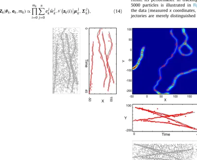
is approximated by a vari-ant of the sequential MCMC scheme described in Section2.2. The respective Matlab code for[22]is available on Matlab Central por-tal[99].

This algorithm presented in Section 2.2and with a likelihood (14)as described above is called a Gaussian mixture MCMC algo-rithm. Its performance in tracking 4 groups using no more than 5000 particles is illustrated in Fig. 6. The top left panel shows the data (measuredxcoordinates, as a function of time). Four tra-jectories are merely distinguished on the background of the noise

[image:8.612.44.445.380.706.2]

(depicted with dots). The upper middle figure shows the estimated xcoordinates (of centers of the groups), obtained with the MCMC-PF. The actual trajectories are depicted via red squares whereas the corresponding estimates are shown as black crosses. The up-per right panel provides contour map plots of the trajectories of the four groups, from the point of view of the sensor. The last two right rows ofFig. 6present, respectively, the estimates of y coordinates for the centers of the four groups and the respective measurements containing a high level of clutter noise.

4.3. Illustrative example on contaminant cloud tracking

The presented Gaussian mixture sequential MCMC technique has been also successfully applied to pollutant cloud tracking in[122]. The tracking of contaminant clouds can also be seen as an extended object tracking problem. The capability to monitor and track contaminant clouds is indeed a problem of great importance. Nowadays, the threat of pollution due to the release, either ac-cidentally or deliberately, of Chemical, Biological, Radiological or Nuclear (CBRN) agents is high. Indeed, many rogue nations and terror groups seek to employ asymmetric warfare and some groups will be attracted by the use of chemical weapons to achieve ma-jor impact. As a consequence, rapid detection and early response to a release of a CBRN agent could dramatically reduce the extent of human exposure.

In[122], the authors propose an inference algorithm within a Bayesian framework to track directly the contaminant concentra-tion, instead of some contaminant boundary as in[69], thus pro-viding more information about the actual situation. More precisely, the concentration of pollutant is expressed in this work using the following parametric function:

C

(x,

y,tk

)

=

N_tk

i=1

wtk,i 2

π

|

Σ

tk,i

|

1/2

e−

1 2([

x

y]−μtk,i)TΣ−_tk1,i([ x

y]−μtk,i)

_.

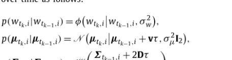
₍₁₆₎

This formulation of the concentration field of interest is moti-vated by two widely used dispersion models: the Gaussian Puff Model and the Gaussian Puff Particle Model. The parameters of each Gaussian shape, involved in Eq. (16) evolve independently over time as follows:

p(wtk,i

|

wtk−1,i

)

=

φ

wtk,i

wtk−1,i

,

σ

2

w

,

(17)

p(

μ

_tk,i

|

μ

_tk−1,i

)

=

N

μ

_tk,i

μ

_tk−1,i

+

v

τ

,

σ

_μ2I2

,

(18)

p(

Σ

tk,i

|

Σ

tk−1,i

)

=

W

_Σ

tk−1,i

+

2D

τ

n

,n

,

(19)

where

φ (.

|

ν

,

σ

2

₎

_{is the truncated normal distribution with mean}

ν

and variance

σ

2 _{defined on}

_[

₀

_,

_+∞

₎

_{to ensure the positivity}

of the weight variable. The mean vector transition probability is a random walk with a linear drift depending on the wind velocityv

and the covariance matrix is assumed to be a Wishart random ma-trix with a scaling mama-trixD

τ

(Dis the pollutant diffusion matrix) and a number of degrees of freedomn.

τ

=

tk

−

tk−1 corresponds

to the sampling interval betweentk andtk−1. As in the previous

example of large group tracking, the problem consists in estimat-ing sequentially the evolution of a sum of dynamic multivariate Gaussian components. The only difference is in the likelihood func-tion.

For chemical, biological or radiological source term estimation, several sensors allow to measure the concentration in the atmo-sphere like the LCAD (Lightweight Chemical Agent Detector) and the MCAD (Mobile Chemical Agent Detector) but one of the most data rich sensors currently available is the LIght Distance And Ranging (LIDAR) sensor. The observations from sensors can be generally

written as a nonlinear function of the concentration field and noises that take into account both the dispersion model uncer-tainty and the measurement error:

Zk

=

f

C

(x,

y,tk

),

vtk

.

(20)

In a Bayesian framework, the aim is thus to compute the poste-rior distribution p

(

{

wk,i

,

μ

k,i

,

Σ

k,i

}

N_tk

i=1

,

Ntk

|

Z1:k

)

wherez1:k is the

observation set from time 1 to tk in order to give estimate of the parameters involved in the concentration field. The main chal-lenging difficulty in this problem is the fact that we have to deal with unknown and time-varying number of Gaussian shapes for the concentration as well as nonlinearity and non-Gaussianity in the model. In[122], the authors propose algorithm to identify and track these multiple contaminant clouds based on a sequential Monte Carlo Markov Chain (MCMC) mechanization which approxi-mates the filtering distribution of interest.

To illustrate the results obtained by this sequential MCMC in this context, the scenario studied in this section consists of one cloud modeled by 3 Gaussian shapes then at time t

=

150 s, an other cloud modeled by one Gaussian puff appears in the obser-vation scene. The synthetic data are generated using the stochastic Gaussian puff model described by Eqs.(17)–(19).

In the sequential MCMC algorithm used to track the contami-nant clouds, all Gaussian shapes are initialized as inactive in order to allow the algorithm to identify all the Gaussian shapes neces-sary to model the actual contaminant clouds. The maximum num-ber of Gaussian shapes in the algorithm is set to Nmax

=

5. For each complete LIDAR scan, 4000 MCMC iterations are performed with burn-in of 1000 iterations. All 4000 MCMC output are kept as particle approximation to posterior distribution.

Fig. 7 illustrates true concentration of the cloud (on the left column), the results from the Gaussian mixture sequential MCMC technique (in the middle column) in time steps respectively 108, 307 and 557 and the measurements obtained with an LIDAR (in the rightmost column).

From this figure it can be recognized that the filtering algorithm is able to adequately identify and track the contaminant clouds in a difficult scenario with heavy clutter.

4.4. The approach with random matrices

A common approach consists in decomposing the joint filtering pdf of groups’ state and extent. Group extent has been modeled by means of symmetric positive definite (SPD) random matrices in [8,75,74,46,45,150]. Attributed to [74,75] it is called the random matrix approach as it considers an augmented state containing the kinematic states and the extent parameters, where the extent is modeled as a random matrix.

In [22] the extent parameters are merely the covariance ma-trices in a Gaussian mixture representation of the groups’ forma-tion. In [8,75,74,46,45] the positive definiteness of the extent is preserved between consecutive time steps by sampling from the inverse Wishart distribution for which the mean is prescribed by the preceding covariance matrix.

In particular, the propagated pdf of the jth group center,

μ

_kj, and extent (SPD matrix),

Σ

_kj, is expressed as

p

μ

_kj

,

Σ

_kj

Z

0:k−1

=

p

μ

_kj

Σ

_kj

,

Z0:k−1

p

Σ

_kj

Z

0:k−1

=

N

μ

_kj

μ

ˆ

_kj

,

Pk

⊗

Σ

_kj

I W

Σ

_kj

ν

k

,

Σ

ˆ

j k

,

(21)

where

I W

denotes the inverse Wishart density with parame-ters

ν

k and

Σ

ˆ

j

k. Here,

μ

ˆ

j k,

Σ

ˆ

j

[image:9.612.43.271.495.554.2]

[image:10.612.137.448.52.294.2]

Fig. 7.The true average concentration of the cloud is shown in log scale (left panel). The estimated average concentration is given in log scale (middle panel). Fluorescences above the threshold in red obtained from a complete LIDAR scan are presented in the right panel. (For interpretation of the references to color in this figure legend, the reader is referred to the web version of this article.)

conjugate prior for the likelihood p

(

Zk

|

μ

_kj

,

Σ

_kj

)

which thereby al-lows deriving a rather elegant filtering recursion for both cluster mean and extent[74,75]. Hence,(21)is known as Gaussian inverse Wishart (GIW) distribution[74,75].

A combination of the random matrices approach [74,46,45] for the group extent and the PHD filter is reported in[58,59,55, 60]. Considering also the Poisson clutter rate unknown, the likeli-hood of the filter proposed in[59,55] is gamma Gaussian inverse Wishart (GGIW) distributed. The gamma distribution is for the clutter term,4 _{and similarly to [74,75], the Gaussian term is for} the kinematic state and the inverse Wishart for the extent. In[85] Cardinality PHD filter for extended targets is proposed which re-laxes the Poisson assumptions of the extended target PHD filter in target and measurement numbers. A GGIW mixture filter is im-plemented and its efficiency in estimating the target extent and measurement rates together with the kinematic state of the target, is demonstrated.

Apart from conjugate priors, other distributions have been recently used in few Bayesian nonparametric tracking methods. A promising trend is to avoid the often restrictive assumptions of parametric models by designing nonparametric models on infinite-dimensional spaces of functions (e.g. with Gaussian pro-cesses [105]) and/or probability distributions (e.g. Dirichlet pro-cesses[47]). In[78,79,134]irregular extended and group targets is considered by the random matrices approach.

A different approach called Histogram Probabilistic Multi-Hypothesis Tracker with Random Matrices (H-PMHT-RM) is sur-veyed in[35,151]. A Wishart prior is applied to the inverse of the appearance covariance matrix. The initially proposed H-PMHT ap-proach deals with Gaussian shaped targets and fixed or known extent.

In the next subsection, we present the Random Finite Set Statis-tics approach which has been shown to be very powerful for the considered problems.

4 _{Remind that in Bayesian inference, the conjugate prior for the rate parameter of}

the Poisson distribution is the gamma distribution.

4.5. Group tracking using random finite sets

In the Bayesian estimation framework the states and mea-surements are treated as realizations of random variables. In the random sets statistics (RSS), known also as Finite Set Statistics (FISST) [86] the targets states and the measurements are con-sidered as random sets with unknown numbers. The number of elements in a random finite set is called the set cardinality. The FISST provides an elegant framework for statistical solutions to the group tracking problems. The FISST affords to detect, identify, track and classify groups of targets. It is a natural framework to deal with interval, stochastic and data association uncertainties. The FISST avoids the direct data association and hence the combina-torial problems due to data association which is one of its major advantages.

For group tracking a hierarchical layer of objects is envisaged, with the lowest layer being the individual target. Such a random-set filtering approach for tracking groups of targets was proposed in [86]. In conventional tracking, the target state space is treated as a hidden layer, where the observation space is visible. For group tracking, the group targets are further treated as a doubly or twice-hidden layer, and each group target is a random collection of some of the targets in the first hidden layer.

In FISST the PHD has the same meaning as the intensity func-tion of a Poisson point process. It is the first moment in point process theory [89,87,146,142,113,116]. The PHD is also regarded as the first-order statistical moment, or expectation, of the multi-target posterior density. Similarly to the Kalman filter where the mean and variance of the posterior state are recursively propa-gated, the PHD filter propagates the PHD function by using similar steps prediction and update, however by means of a different and more complicated procedure. The integral over the PHD in a region gives the expected number of targets in that region. Hence, the es-timated states of the targets can be inferred from the peaks of the PHD.

[image:11.612.163.447.59.224.2]

Fig. 8.Large groups, their extents and intensity functions. The top left and middle figures show the intensity functions of two and three groups, respectively. The figures on the second row show groups represented by ellipses. The groups’ extent is characterized by the centers and axes of the ellipses. The last row illustrates the peaks of the intensity functions. Typical splitting and merging moves are illustrated in the rightmost panels.

measurements as random finite sets. A random finite set[146]is simply a random variable which values are unordered random sets. The multi-target evolution and observation models are considered under the following assumptions: (i) Each target evolves and gen-erates observations independently of one another; (ii) The birth random finite set and the surviving random finite sets are indepen-dent of each other; (iii) The clutter random finite set is of Poisson type and independent of target originated measurements; (iv) The prior and predicted multi-target sets are with a Poisson distribu-tion.

Instead of working with pdfs, the PHD filter updates recursively the intensities for the prediction and measurement update, respec-tivelyvk|k−1 andvk|k:

vk|k−1

(

X

)

=

pS,k

(ζ )

fk|k−1

(

X

|

ζ )v

k−1

(ζ )

dζ

+

γ

k

(

X

),

(22)

where fk|k−1

(

X

|

ζ )

is the group transition density at timek,pS,k

(ζ )

is the group survival probability and

γ

k

(

X

)

is the intensity of spon-taneous birth. The update equation is given by

vk|k

(

X

)

=

1

−

pD,k

(

X

)

vk|k−1

(

X

)

Non-detected targets

+

zk∈Zk

pD,k

(

X

)

gk

(

zk

|

Xk

)v

k|k−1

(

X

)

κ

k

(

zk

)

+

pD,k

(ξ )g

k

(

zk

|

ξ )v

k|k−1

(ξ )

dξ

Detected targets

,

(23)

wheregk

(

zk

|

Xk

)

is the group measurement likelihood, pD,k is the probability of group detection, and

κ

k

(

zk

)

is the intensity of clutter measurements. The first part of(23)corresponds to non-detected targets and the second term of(23)to the detected targets. Practi-cal implementations of the PHD filter include two main implemen-tations: the SMC solutions [142] and Gaussian mixtures [144,86, 57,30,29]. The SMC implementation of the PHD filter approximates the set integrals by propagating a large set of weighted particles over time. The sum of the weights of the particles represents the expected number of targets since the integral over the PHD is the expected number of targets. An improved SMC PHD approach is proposed in[115] which adapts the target birth intensity at each processing step using the received measurements.

The alternative GM PHD implementation approximates the PHD with a mixture of Gaussian distributions and uses Kalman filters or their nonlinear variants such as Unscented Kalman filters[70].

Various approaches are proposed to deal with the unknown number of targets within each group, such as using the birth–

death model[109] and estimate the unknown number of targets within each group or the Cardinality PHD (CPHD) filter which es-timates the number of targets jointly with the kinematic states. In [93] a step further is done where the cardinality number is estimated with the states, together with the clutter noise param-eters and probability of detection. This is a general formulation affording to resolve state and parameter estimation problems si-multaneously.

The relation between the underlying group shape and entity concentrations is represented via intensity functions [89]. The in-tensity function indicates how entities are situated in the state space (i.e., the peaks correspond to the most dense regions in the state space). This is illustrated in Fig. 8. The top left and middle figures show the intensity functions of two and three groups, re-spectively, depending on xand y coordinates of the group center. The middle row figures show the groups, represented by ellipses. The last row shows the intensity function in which each peak cor-responds to a group. Group splitting and merging are illustrated in the right panels. These are reflected in the changes of the number of peaks of the intensity functions.

In [132,133,124,126] a different approach is proposed based on the Poisson Point Processes (PPPs). However, the algorithm in essence is similar to the PHD filter.

FISST[89,143]and cluster point processes [33,131]are natural mathematical frameworks for analyzing group target motions and extended targets. In general, a cluster process is described as a su-perposition of point processes. The cluster centers can form parent point processes and their associated component points can form daughter point processes. This layering process can continue up-wards, forming groups of groups. In principle such a formulation is general enough to deal with multiple layers of interactions. The multi-group multi-target multi-sensor density can then incorporate group dynamics and group likelihoods. While this is general, it will be a challenge to model the actual interactions between groups of groups.