Numerical Implementation and Test of the Modified Variational Multiconfigurational Gaussian Method for High-Dimensional Quantum Dynamics

This is a repository copy of

Numerical Implementation and Test of the Modified Variational

Multiconfigurational Gaussian Method for High-Dimensional Quantum Dynamics

.

White Rose Research Online URL for this paper:

http://eprints.whiterose.ac.uk/88797/

Version: Accepted Version

Article:

Ronto, M and Shalashilin, DV (2013) Numerical Implementation and Test of the Modified

Variational Multiconfigurational Gaussian Method for High-Dimensional Quantum

Dynamics. Journal of Physical Chemistry A, 117 (32). pp. 6948-6959. ISSN 1089-5639

https://doi.org/10.1021/jp310976d

© 2013 American Chemical Society. This document is the Accepted Manuscript version of

a Published Work that appeared in final form in Journal of Physical Chemistry A, copyright

© American Chemical Society after peer review and technical editing by the publisher. To

access the final edited and published work see http://dx.doi.org/10.1021/jp310976d.

Uploaded in accordance with the publisher's self-archiving policy.

[email protected] https://eprints.whiterose.ac.uk/

Reuse

Unless indicated otherwise, fulltext items are protected by copyright with all rights reserved. The copyright exception in section 29 of the Copyright, Designs and Patents Act 1988 allows the making of a single copy solely for the purpose of non-commercial research or private study within the limits of fair dealing. The publisher or other rights-holder may allow further reproduction and re-use of this version - refer to the White Rose Research Online record for this item. Where records identify the publisher as the copyright holder, users can verify any specific terms of use on the publisher’s website.

Takedown

If you consider content in White Rose Research Online to be in breach of UK law, please notify us by

1

Numerical Implementation and Test of the Modified Variational

Multiconfigurational Gaussian Method for High-dimensional

Quantum Dynamics

Miklos Ronto and Dmitrii V. Shalashilin1

School of Chemistry, University of Leeds, Leeds LS2 9JT, UK

Abstract

In this paper a new numerical implementation and a test of the modified variational Multiconfigurational Gaussian (vMCG) equations are presented. In vMCG the wave function is represented as a superposition of trajectory guided Gaussian Coherent States and the time derivatives of the wave function parameters are found from a system of linear equations, which in turn follows from the variational principle applied simultaneously to all wave function parameters. In the original formulation of vMCG the corresponding matrix was not well behaved and needed regularisation, which required matrix inversion. The new implementation of the modified vMCG equations seems to have improved the method, which now enables straightforward solution of the linear system without matrix inversion, thus achieving greater efficiency, stability and robustness. Here the new version of the vMCG approach is tested against a number of benchmarks, which previously have been studied by split-operator, Multiconfigurational Time Dependent Hartree (MCTDH) and Multilayer MCTDH (ML-MCTDH) techniques. The accuracy and efficiency of the new implementation of vMCG is directly compared with the method of Coupled Coherent States (CCS), another technique which uses trajectory guided grids. More generally we demonstrate that trajectory guided Gaussian based methods are capable of simulating quantum systems with tens or even hundreds of degrees of freedom previously accessible only for MCTDH and ML-MCTDH.

I INTRODUCTION

Exact analytical solvability of the time-dependent Schrödinger-equation for systems with large

number of degrees of freedom (DOF) is limited to a few simple models. There are two problems

which make multidimensional quantum mechanics difficult to deal with. First, determining the

potential energy surface is a complicated problem, which is also present in classical molecular

dynamics. Recently substantial progress has been made1, 2 _{with various forms of PES parametrisations}

and fits. The second problem is the scaling of quantum mechanics with the number of degrees of

freedom (DOF): the number of quantum states increases exponentially with the size of quantum

system. Impressive progress has been made in calculations of quantum states for the systems

comprised of large numbers of coupled vibrational modes3some of which can be very “floppy”3, 4_{. In}

dynamical calculations – when evolution of the wave packet is not restricted to a certain area – the

“exponential curse” of quantum mechanics is perhaps the most severe. If a static grid of states is used for a single-mode, a problem of DOF requires

2

(1.1)

grid points making the challenge of exponential scaling almost insurmountable.

In the last few decades a family of concepts based on trajectory guided Gaussians, which rely on

locally defined adaptable basis sets, gained considerable importance. A number of methods both

semiclassical and formally exact have been developed. The list of most important techniques can be

divided into two categories. Semiclassical methods include but not limited to the early application of

Frozen Gaussians5 _{and semiclassical Herman-Kluk propagator}6, 7_{. For more details and new}

developments of the semiclassical Gaussian based methods see review8_{. Fully quantum techniques}

which at least in principle can be converted to fully quantum result include Multiple Spawning9_,

Gaussian Multiconfigurational Time Dependent Hartree (G-MCTDH10_{), Coupled Coherent States}

CCS11-13_{, variational Gaussian approach}14 _{and variational Multiconfigurational Gaussians (vMCG)}15_.

All these techniques use grids (or basis sets) of trajectory guided Frozen Gaussian Coherent States,

which follow the wave function thus economising the basis set size. Another advantage of such

techniques is that a randomly sampled basis can be used, which is advantageous in high dimensional

problems because Monte Carlo techniques scale with dimensionality much better than (1.1).

Importance sampling, which is the crucial part of all above methods, allows the basis to be built only

around the dynamically important phase-space region. With such random sampling the Gaussian based

methods can potentially scale as , although in reality the scaling is often worse than that. However,

even with the ever increasing computational power, the methods based on trajectory guided Gaussians

sometimes suffer from two difficulties: scaling and robustness.

Variational Multiconfigurational Gaussians10, 15 _{(vMCG) is potentially one of the most efficient}

methods of high dimensional quantum dynamics. In vMCG the wave function is represented as a

superposition of N trajectory guided Gaussian wave packets

(1.2)

The time evolution of the wave function can be determined from the variational principle. It yields time

derivatives of its parameters which can be obtained from a system of linear equations

(1.3)

where is the vector of wave function parameters, which includes both the amplitudes and all

positions of N coherent states (each one of them M-dimensional ) and is the

matrix which can be derived for example using the elegant formalism developed by Kramer and

Saraceno16 _{(See Ref}17 _{for more details). Matrix D in (1.3), as well as similar matrices in other}

variational approaches18-21_{, is often numerically nearly singular and has to be regularised. This may be}

done by matrix inversion, during which the lowest eigenvalues of D are increased by a small and

somewhat arbitrary regularisation parameter so that the inverse matrix does not have extremely large

elements. As a result the equation is eventually written as

(1.4)

which is of course equivalent to (1.3) from the formal point of view. Numerically however matrix

3

equations of the Couple Coherent States (CCS) technique12_{, another method based on trajectory guided}

Gaussians. In CCS special efforts were made to minimise coupling between the amplitudes by making

the coupling matrix small, smooth and sparse. CCS introduces a preexponential factor to smooth out

the rapid oscillations of quantum amplitudes. It appears that this simple trick works also for vMCG and

makes matrix D sufficiently well behaved. In the tests of the vMCG equations17 _{presented here we}

were able to solve the equations (1.3) without inverting the matrix. Since our version of vMCG is

closely connected to the CCS theory we also compare accuracy and efficiency of the two techniques.

With the same basis size vMCG is more accurate simply because it employs more variational

parameters, as the time dependence of all the parameters in (1.2) are determined variationally. For the

same number of variational parameters however the accuracy of the two techniques is close and both

methods show similar levels of robustness and stability.

In the Chapter II we briefly sketch our version of the vMCG theory, which in the original paper17

was presented for 1D case only. Here we present the theory in multidimensional form, which is

conceptually simple but involves long algebra, given in the Appendix A1. Chapter III provides details

of the numerical tests. First, our implementation of vMCG was tested on simple Morse oscillator

because a 1D problem allows to visualise complicated variational trajectories. Then Henon-Heiles

(HH) model was investigated and the accuracy and efficiency of vMCG was compared with those of

CCS, using MCTDH benchmark obtained previously for 2D, 6D, 10D and 18D Henon-Heiles

systems22_{. To demonstrate the limitations of vMCG and its scaling with the number of degrees of}

freedom we also performed CCS calculation for 1458D model previously studied in the ref23 _by

ML-MCTDH, and show that vMCG calculation for a system of such size is not feasible but CCS yeilds a

good result. We also use this example to make some general remarks about the accuracy and

convergence of vMCG, CCS and MCTDH, ML-MCTDH methods24 _{of high-dimensional quantum}

mechanics.

Throughout this paper natural units were used with , and the Coherent States were set to have

a�d

II THEORY 2.1 Coherent states

Coherent state (CS) based approaches gained considerable importance in molecular dynamics. As they

are minimum uncertainty states and Gaussian-functions they are compatible with both semiclassical

and quantum mechanical descriptions. A single-mode coherent state z is an element of the phase-space

where qi and pi are canonically conjugated variables. Using phase-space coordinates a 1D

coherent state can be written as

(2.1)

4

(2.2)

with , where z and z* _{are eigenstates of the annihilation and creation operators:}

(2.3)

(2.4)

A multidimensional CS is a product of m single-mode CSs

(2.5)

and represents a point in M-dimensional phase space The overlap of

two M-dimensional CS’s

exp

exp

(2.6)

is a product of M 1D overlaps. Although continuum basis of coherent states is overcomplete in

numerical calculations we always deal with a finite set of CSs which simply represent a non-orthogonal

basis with the overlap matrix (2.6). In this finite basis of Coherent States the identity becomes

(2.7)

where are the elements of the inverse overlap matrix of CSs. The identity (2.7) is a discretisation

of that of the continuous manifold covering all z-space where is the product of M 1D integral

identities

(2.8)

with the single-mode integral measure . For more details about CS notations refer to Ref.12_.

With the coherent state representation any time-dependent wave function and its conjugate can be

written up in coherent state basis in the general form (1.2). In coordinate representation a CS is simply

a multidimensional Gaussian wave packet with the following ansatz

exp (2.9)

Matrix elements of an arbitrary operator can be found via its normal ordered form in

which the powers of the creation operator precede those of the annihilation operator if are

5

This is also applicable to the single mode Hamilton operators:

(2.11)

The index “ord” simply reminds about the terms which originated from commuting . The Hamilton operator of the system is the sum over the dimensions of the individual single-mode

Hamiltonians and their coupling terms:

(2.12)

2.2 Dynamics

Time dependent variational principle (TDVP) provides a generic way to derive various forms of the

time-dependent Schrödinger-equation. Several formulations of TDVP exist16, 18-21_{; our description here}

is based on the approach16 _{where TDVP is presented in a form similar to the principle of least action in}

classical mechanics and defining equations of motion through Euler-Lagrange equations. According to

the principle of least action, the equations of motion can be obtained from the extremum of the

functional

(2.13)

where the Lagrangian is

(2.14)

with the differential-operator acting separately on bras and kets. Any state vector can be

rewritten in coherent state form (1.2) t t t , and therefore the Lagrangian can be

reparametrised with amplitudes and coherent states phase space positions as17_:

(2.15)

Where is the vector of the wave function parameters which includes all N× M components of

the M-dimensional complex vectors describing the phase space positions of all basis coherent

states and N their amplitudes . Quantum equations of motion can now be written as standard

Lagrange equations for the wave function parameters

d

dt (2.16)

which after introduction of a conjugated momentum can be presented in the form of

6

(2.17)

where D is the matrix with the elements and is the effective Hamiltonian obtained from

the Lagrangian (2.14) in the usual way as . The operator should not be confused

with the actual physical Hamiltonian of the system. The Lagrangian and the effective Hamiltonian

are simply a tool to formally work out the quantum equations of motion. We have used Greek

letters to denote general momentum, action and Lagrangian associated with it to distinguish

them from p, S and L the momentum, action and Lagrangian of the actual trajectory of a physical

coordinate q. More details about the equations and their derivation can be found in17 _{and in Appendix}

A1. Here we only point out that equations17 _{have been written not for the oscillating amplitude}

exp (2.18)

but for smooth preexponential factor , where is the action along the trajectory. As a result matrix

D in (2.17) has many small elements and therefore sparse and smooth.

In vMCG at each time step one has to find the derivatives of the parameters from the system of

coupled N× (M+ 1) linear equations (2.17), where N is the basis set size and M is the number of degrees

of freedom. Coupled Coherent States (CCS) is another method, which utilises exactly the same

parametrisation of the wave function (1.2) as vMCG. The difference is that in CCS the trajectories

are predetermined and calculated from essentially classical equations of motion. Only N

amplitudes are found from a quantum variational principle. As a result the system of linear

equations for the derivatives of is much smaller and much simpler than in vMCG. Matrix D

used in vMCG has the size of [N× (M+ 1)] × [ N× (M+ 1)] and includes that of CCS as a small N× N

block. The elements of this small N× N matrix are simply those of the overlap matrix multiplied by the

exponentials of the classical actions. CCS trajectories are driven by a classical Hamiltonian with

quantum corrections Eq.(2.12), which is simply the expectation value of the classical

Hamiltonian with the Gaussian CS. The mathematical structure of the two methods has been compared

in17_{. In this paper we compare their computational cost and accuracy. At the first glance vMCG appears}

more expensive than CCS. However, as it will be shown below that as vMCG works with a smaller

basis than CSs, the computational cost of the two related methods is comparable.

III NUMERICAL IMPLEMENTATION AND RESULTS 3.1 Basis set sampling

First we have tested vMCG in the form given in17 _{on the examples of 1D harmonic and 1D Morse}

oscillators. Then we employed multidimensional Henon-Heiles model in 2D, 6D, 10D, 18D and

1458D. The results were compared with CCS and with the benchmarks provided earlier by MCTDH22

and ML-MCTDH23_{. Since both CCS and vMCG utilise the grids of trajectory guided coherent states}

we also compare their accuracy and efficiency. In both CCS and vMCG methods the initial propagating

7

In both approaches the sampling of the Gaussian Coherent State basis is very important and we have

used the same techniques suggested previously in11 _{to select initial conditions for the basis set .}

The simplest way to bias the basis to the dynamically important region would be to use the

“compressed swarm”. The initial phase space positions of CSs have been chosen randomly from a Gaussian distribution centred around

exp (3.2)

Then the initial amplitudes of are calculated by applying the identity (2.7) as follows

(3.3)

In (3.2) the “compression” parameter determines the degree of bias of the basis set to its centre . The smaller is the basis set, the more compressed the distribution should be. Parameter is chosen

such that the norm of the wave function

_(3.4)

is close to 1, which is not the case for a small basis which is not “compressed” well enough. The norm

was always kept in the range between 0.990 and 0.995. With the sampling discussed above, the

two methods (CCS and vMCG) can be compared on equal footing. The sampling described above is

called Sampling 1 (S1) and used for the majority of the tests.

We also tried another sampling called S2, where the propagating CS was

included into the basis, such that the first basis function is

(3.5)

The rest of the basis was chosen randomly as in the sampling S1. In sampling S2 the initial conditions

for the amplitudes are if and if . These conditions are further described in

Appendix A2.

Another type of sampling strategy (S3) was used for the 1458D Henon-Heiles model where

only two modes are excited initially and the rest of the modes are act like a “bath”. For a multidimensional initial wave function for every mode k a different compression parameter

can be chosen, therefore different compression can be applied for the excited “system” modes and

for the “bath” modes. This allows to treat more important modes with less compression and therefore

with less bias. This sampling strategy is called “pancake” distribution and has successfully been used

for CCS previously11, 25 _{In the 1458D Henon-Heiles system investigated, two adjacent modes (}

and ) are excited in the middle of the chain for these modes no compression was applied in the

sampling (i.e. ). For the “bath” modes the compression was applied according to

8

exp

(3.6)

where parameter gives the width of the discrete Gaussian distribution. Geometrically this means that

the compression rapidly increases for the sampling of less important “bath” modes which are far from

the excited modes and .

3.2 Harmonic oscillator and 1D Morse oscillator

For the Harmonic oscillator both CCS and vMCG give exact solution and their amplitudes and

trajectories are identical. This is due to the fact that with the Hamiltonian of the harmonic oscillator

vMCG equations are equivalent to CCS equations. The simple 1D Hamiltonian of a Morse oscillator

exp exp (3.7)

with the energy parameter , the parameter and initial condition at

, has also been investigated. This system has been previously used to

test CCS26, 27 _{and other related techniques. Methods like vMCG and CCS are suited for high}

dimensional problems and for a 1D problem coherent state based methods do not have advantages

before standard techniques. Moreover if the CS basis becomes too large (which is often just few tens of

CSs) the overlap matrix in CCS and matrix D of vMCG become singular making propagation

numerically unstable. This challenge justifies using simple 1D Harmonic and Morse oscillator models

as a test problem. Also a 1D problem allows to visualise complicates vMCG trajectories. Fig 1 shows

the autocorrelation function obtained by the vMCG method and compares it with that of numerically

exact Split-Operator propagation. Fig 2 shows the guiding trajectories from vMCG methods, which are

very different from those of classical mechanics and almost classical CCS trajectories. The quantum

vMCG trajectories are “pushed” by each other and by their amplitudes.

We found that for the sampling S1 the equations of vMCG17 _{produce an accurate}

autocorrelation function without matrix inversion and regularisation. For sampling S2 when

propagation of the CS is included into the basis and all initial amplitudes except one are zero the

vMCG system of linear equations is not well defined and the propagation is numerically unstable.

Inspection of the matrix D reveals the presence of rows and columns with all elements equal to zero

(Appendix A2), which makes its determinant zero. This has also been noted for the standard

implementation of vMCG15_{. Propagation with the CCS method is stable for both sampling S1 and S2.}

For the S1 sampling vMCG propagation for 1D Harmonic and Morse oscillators worked with the same

time step as CCS and therefore the new version of vMCG was as robust and as stable as CCS. In the

case of sampling S2 vMCG can be made free of numerical instabilities by either regularising the matrix

at the first step as it has been done in the Ref15 _{or by propagating the system with CCS for a few steps}

9

Multidimensional Henon-Heiles (HH) potential with strong coupling between the modes provides a

more challenging benchmark for vMCG and other methods of high dimensional quantum mechanics.

The potential

(3.8)

is multidimensional, anharmonic, unbound and includes coupling terms between the modes with the

coupling constant . The vMCG calculations were compared with CCS for 2D, 6D and

10D and 18D HH systems. In the 2D case comparison can be made with the split-operator method,

while 6D and 10D results can be compared with the benchmark MCTDH22 _{and CCS calculations. In}

the case of 18D model ML-MCTDH benchmark is available23 _{for the standard HH model and the}

“strong coupling” model with coupling constant twice that of the standard parameter

. In addition the ref23 _{reported a calculation for 1458D Henon-Heiles model. HH model}

previously was also used to test semiclassical Gaussian based techniques28, 29_.

For 2D, 6D and 10D models the initial conditions were the same for both CCS and vMCG: the

initial state is placed at (i.e. initially all modes are

stretched and have zero momentum). Those basis Coherent States which become so energetic that they

escape to the distance q> 10 were automatically removed from the calculations. The Figures 3-8 show

the real part of the autocorrelation function (ACF) for 2D, 6D and 10D Henon-Heiles potential.

For the 2D model the time step of vMCG propagation was reduced to to be able to

run it stably, while CCS was still robust with in all the cases. Therefore vMCG can be less

stable for lower dimensional systems (1D or 2D) but reducing time step solves the problem and it still

works well. For the basis set size used (i.e. 100) the result of vMCG is visibly better than that of CCS.

However CCS improves if the basis is increased to 300 CSs such that the number of variational

parameters for both methods is the same.

For both vMCG and CCS we observed similar behaviour in 6D and 10D cases shown at the

figures 4-8. Running time was with timestep of for both cases of CCS and

vMCG. The initial norm was kept close to by setting the compression parameter. For

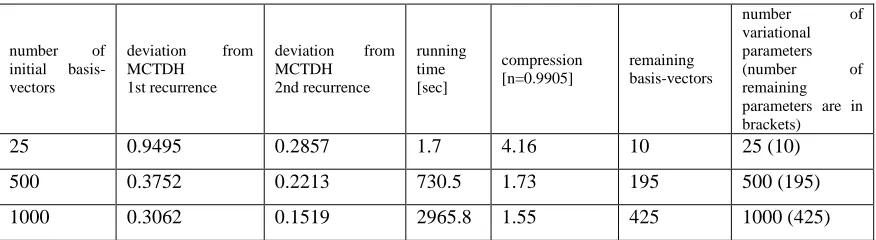
the 10D case we compared the deviation of vMCG and CCS from the MCTDH result. To quantify the

quality of propagation for the 10D case the deviation from benchmark MCTHD was calculated for the

first (Fig. 6-7) and the second recurrence (Fig. 8) for both CCS and vMCG. The comparison of the

results can be seen in Table 1 and Table 2 respectively. Deviation is defined as the square root of the

integral of the square modulus of the difference between the real parts of the two autocorrelation

functions. The conclusion is that for the same number of variational parameters both CCS and vMCG

perform on the same level of accuracy. In high dimensional 6D and 10D cases the time step was the

same for both vMCG and CCS and vMCG performance was sufficiently robust and stable.

Two different 18D HH systems were investigated and the results are shown on Figures 9-11,

which present the absolute value of the autocorrelation function. The first system had the coupling

10

stronger coupling increased by the factor of 2. Only the modes 4, 8,12 and 16 were

excited in both the standard and

stronger coupling cases. For 18D HH simulations running time was and the time step had

to be reduced to for CCS and for vMCG. The initial norm was set with the

compression parameter to be close to . The results of the standard and strong coupling

can be seen in the Figures 9-11. These results were compared with ML-MCTDH simulations23 _(Fig.

9a) and (Fig. 10a). For CCS 3000 basis vectors were used, while in the case of vMCG the basis set size

was 150 Coherent States, however essentially the same result can be obtained with 1000 CSs for CCS

and 50 CSs for vMCG (frame (b) on Figures 9-10) so that both vMCG and CCS calculations were well

converged. The strongly coupled Henon-Heiles model is a more demanding problem: after a few

oscillations the autocorrelation function decays so rapidly that it almost vanishes. On Fig. 11 the CCS

and vMCG results are shown, compared with ML-MCTDH results. Although a relatively large basis

set was used – 4000 CSs for CCS and 200 for vMCG – the running time of the simulation was shorter

compared to the previous case of standard HH model. This is due to the trajectories of the basis

Coherent States escaping from the well of the Henon-Heiles potential and being removed from the

propagation. By the end of the propagation only 300 CSs were left in the case of CCS and only 8 for

vMCG, making the basis very small. The quality of basis can be easily improved by generating new

basis functions instead of escaping ones, but we have not done it in this work. As can be seen from the

figure 11 even a very small basis provides quite accurate result where the autocorrelation function is

not very small.

Since the HH 1458D benchmark result was available for the 1458D Henon-Heiles model23 _we

endeavoured to attempt similar calculation with vMCG and CCS methods. In ref23 _{two cases of 1458D}

HH model were investigated. In the first case, called System 1, only the modes 486 and 487 were

initially excited to . In the second case called System 2

only the modes 729 and 730 were stretched as . In both

systems the excited modes are in the midle of the chain of coupled oscillators and far from its ends.

Thus, our expectation is, that the results from the two exact propagations should lie very close to one

another. The difference between the two cases is that for the System 1 the mode combination in not

good. Quoting the ref23_{, System 1} “represents an example of the wrong _choice of tree structure” in

ML-MCTDH. On the contrary the mode combination and ML-MCTDH tree structure for the System 2

is correct. Simulations of the 1458D Henon-Heiles model would be very time consuming for vMCG

albeit not impossible. Even a basis set as small as 5 Gaussian Coherent Sets would include

1458×5+5=7295 variational parameters which would require the solution of a system of 7295 linear

equations (1.3) for derivatives of the parameters. On the other hand CCS was able to tackle this very

high dimensional problem, yielding the results shown on Figures 12-14 for the basis of 500CSs

sampled with Sampling S3. Sampling S1 gives similar result. Fig.12 shows that CCS autocorrelation

function deviates from that of ML-MCTDH for the System 1 very quickly, but agreement for the

System 2 is much better. Figure 13 indicates that for the System 2 the first two recurrences are in good

agreement with ML-MCTDH. Unlike ML-MCTDH results from CCS for System 1 and System 2 are

11

CCS basis always deteriorates because a) the Coherent States run away from each other and eventually

stop exchanging amplitudes, and b) CCS trajectories may guide basis in the wrong place. As a result,

at longer times CCS works as a semiclassical technique. Good sampling of the basis set is crucial for

the efficiency and convergence of CCS and the same can be said about vMCG or any other trajectory

based method. MCTDH is also a short time method and it provides accurate results only if appropriate

mode combination is found.

V CONCLUSIONS

In this paper the numerical implementation of the modified vMCG equations was discussed. The

results are directly compared with the results obtained by CCS on equal formal footing. The tests and

comparisons have been made for 1D harmonic, 1D Morse oscillator and for 2D, 6D, 10D and 18D

Henon-Heiles models. For the same basis set size vMCG is more accurate but for the same number of

variational parameters the quality of vMCG and CCS propagations is similar. Convergence and

efficiency of CCS has been investigated previously and the modified vMCG method shows very

similar numerical behaviour in terms of convergence of results and norm-conservation. The main result

of this paper is that for the test systems considered here our implementation of the modified version of

vMCG equations works without regularising and inverting the matrix D in Eq.(1.3), which significantly

reduces computational costs.

It is interesting to discuss the future of various trajectory based methods for quantum molecular

dynamics simulations where “on the fly” ab-initio dynamics is the current trend. Many ab-initio techniques such as Multiple Spawning (AIMS)9, 30_{, Multiconfigurational Ehrenfest dynamics (MCE)}31_,

which is a generalisation of CCS, and “on the fly” implementation of vMCG exist32, 33_{. In such} methods the potential energy surfaces are calculated by applying an electronic structure package along

the trajectory, which is the most expensive part of calculations. Having fewer vMCG trajectories may

therefore have an advantage over the methods which use predetermined trajectories. On the other hand

methods like CCS/MCE allow the running of trajectories one by one independently from each other

which is not possible in vMCG, where trajectories are coupled with each other. Independent

trajectories allow a detailed exploration of the dynamically relevant part of the PES prior to actual

quantum dynamics calculation. Many electronic structure points can be accumulated and fit with the

modern algorithms1, 2_{. Perhaps a combination of vMCG and techniques which use predetermined}

trajectories will provide an optimum solution in the future.

Acknowledgement

This work has been supported by EPSRC grants EP/I014500/1 and EP/J001481/1. We thank Irene

Burghardt and Graham Worth for useful discussions, Mathias Nest for providing the MCTDH

benchmark data, Hans-Dieter Meyer for providing the ML-MCTDH results and Christopher Symonds

12

REFERENCES

1

J. M. Bowman, B. J. Braams, S. Carter, C. Chen, G. Czako

, B. Fu, X.

Huang, E. Kamarchik, A. R. Sharma, B. C. Shepler, Y. Wang and Z. Xie, The Journal

of Physical Chemistry Letters, 1, 1866-1874.

2

J. M. Bowman, G. Czako and B. Fu, Physical Chemistry Chemical Physics, 13,

8094-8111.

3

J. M. Bowman, S. Carter and X. Huang, International Reviews in Physical

Chemistry, 2003, 22, 533-549.

4

J. M. Bowman, T. Carrington and H.-D. Meyer, Molecular Physics, 2008, 106,

2145-2182.

5

E. J. Heller, J. Chem. Phys., 1981, 75, 2923-2931.

6

M. F. Herman and E. Kluk, Chemical Physics, 1984, 91, 27-34.

7

M. S. Child and D. V. Shalashilin, J. Chem. Phys., 2003, 118, 2061-2071.

8

K. G. Kay, in Annual Review of Physical Chemistry, Annual Reviews, Palo

Alto, 2005, vol. 56, pp. 255-+.

9

M. Ben-Nun and T. J. Martinez, Advances in Chemical Physics, Volume 121,

2002, 121, 439-512.

10

I. Burghardt, H. D. Meyer and L. S. Cederbaum, J. Chem. Phys., 1999, 111,

2927-2939.

11

D. V. Shalashilin and M. S. Child, J. Chem. Phys., 2008, 128, 054102-054102.

12

D. V. Shalashilin and M. S. Child, Chemical Physics, 2004, 304, 103-120.

13

D. V. Shalashilin and M. S. Child, J. Chem. Phys., 2001, 115, 5367-5375.

14

S. I. Sawada, R. Heather, B. Jackson and H. Metiu, J. Chem. Phys., 1985, 83,

3009-3027.

15

G. A. Worth and I. Burghardt, Chemical Physics Letters, 2003, 368, 502-508.

16

P. Kramer and M. Saraceno, Geometry of the Time-Dependent Variational

Principle in Quantum Mechanics NewYork, 1981.

17

D. V. Shalashilin and I. Burghardt, J. Chem. Phys., 2008, 129.

18

J. Frenkel, Wave Mechanics, Advanced General Theory, Clarendon Press,

Oxford, 1934.

19

J. Broeckhove, L. Lathouwers, E. Kesteloot and P. Vanleuven, Chemical

Physics Letters, 1988, 149, 547-550.

20

K. G. Kay, Chemical Physics, 1989, 137, 165-175.

21

A. D. McLachlan, Molecular Physics, 1964, 8, 39.

22

M. Nest and H. D. Meyer, J. Chem. Phys., 2002, 117, 10499-10505.

23

O. Vendrell and H. D. Meyer, J. Chem. Phys., 2011, 134, 044135.

24

G. F. Meyer H.-D., Worth G.A. ed., Multidimensional Quantum Dynamics.

MCTDH Theory and Applications, Wiley-VCH, 2007.

25

P. A. J. Sherratt, D. V. Shalashillin and M. S. Child, Chemical Physics, 2006,

322, 127-134.

26

D. V. Shalashilin and M. S. Child, J. Chem. Phys., 2000, 113, 10028-10036.

27

D. V. Shalashilin and B. Jackson, Chemical Physics Letters, 2000, 318,

305-313.

28

T. Sklarz and K. G. Kay, The Journal of chemical physics, 2004, 120,

2606-2617.

29

M. L. Brewer, J. Chem. Phys., 1999, 111, 6168-6170.

13

31

K. Saita and D. V. Shalashilin, The Journal of chemical physics, 2012, 137,

22A506-508.

32

G. A. Worth, M. A. Robb and B. Lasorne, Molecular Physics, 2008, 106,

2077-2091.

14

A

A1 Working equations of modified vMCG

Derivation of the equations of motion for from the time-dependent variational principle

enables us to investigate CCS and vMCG on the same formal footing. The Euler-Lagrange equations

(2.16) for dynamic parameters and can be obtained separately from the Lagrangian (2.15)

as

d

dt and

d

dt (A1.1)

Performing the variation for amplitudes gives

(A1.2)

and the variation of is

.

(A1.3)

For the sake of greater stability and better robustness it is convenient to introduce a smoothing

preexponential factor to describe the rapidly oscillating amplitudes :

exp (A1.4)

where can be calculated from the classical action:

(A1.5)

With this preexponential factor equation (A1.2) can be rewritten as

exp exp

exp (A1.6)

15

exp

exp

exp

(A1.7)

The time evolution of can be described by solving the equations for , and . In

the case of CCS the equations of motion for are given by Hamilton’s equations:

(A1.8)

This can be obtained from (A1.6) if all terms containing small overlaps between different coherent

states are neglected. In CCS the equations for the amplitudes (preexponential factors) are still the same

as (A1.6). Although the trajectories (A1.8) are not fully variational the CCS technique is still fully

quantum because it relies on the exact coupled equations for the amplitudes. It has been shown in CCS

that better stability is achieved by smoothing the amplitude by (A1.4). In vMCG both fully variational

equations (A1.5) and (A1.6) are used, these are in principle equivalent to those of original vMCG

theory15_{. The equations are forming a system of linear equations for the dynamical variables and}

:

(A1.9)

where

(A1.10)

This set of linear equation can be written in matrix form as

(A1.11)

where in this block matrix every letter represents an matrix with the following elements:

exp

exp

exp

exp

exp

16

exp

(A1.12)

The only improvement is that they are written for the smooth preexponential factor d rather than for the

amplitude itself. Although an attempt has been made in the original vMCG15 _{to take oscillating part}

away from the amplitude the exact way of how this should be done can be important. In the current

formulation the smoothening is done in a fashion similar to the CCS technique and the matrix D

appears to be small, smooth and sparse and reasonably well behaved.

Numerically CCS can be implemented easier than vMCG. The two differences in the program code are

the way and are calculated and the derivative matrix of the Hamiltonian. The structure of the

working matrix of CCS is simpler as it contains coefficients for only, thus it is independent of the

dimension of the system. The other significant difference is that CCS uses only the diagonal elements

of the derivative of the Hamiltonian, whereas for vMCG all the elements for all dimensions have to be

calculated.

A2 Numerical instabilities of Sampling S2

Let us set one of the initial CS to such as in (3.5)

(A2.1)

Then the initial amplitude is

(A2.2)

and the overlap-matrix will be:

. (A2.3)

Amplitude d is calculated from the set of linear equations

(A2.4)

17

a�d (A2.5)

The initial action and therefore exp With these conditions the components of matrix

D and vector b in equations (A1.11) will be as follows:

if a�d elsewhere

if a�d elsewhere

if a�d elsewhere

if a�d elsewhere

if a�d elsewhere

(A2.6)

It can be seen, that in matrix D every th column and every th row

contains zeros only. This makes D singular, although the matrix is not inverted; therefore the problem with det is still solvable. The under-determined system of linear equations in the case of vMCG will lead to numerical difficulties which requires regularisation. In the case of CCS only D1 and b1 are calculated; this system has unambiguous solutions.

18

Figures

Fig.1 Real part of the autocorrelation function of a 1D Morse-potential given by vMCG with the basis set size of 10 Gaussians (solid line), compared results from Split-Operator method (crosses)

Fig.2 Typical complicated quantum variational trajectories of a 1D Morse-potential with vMCG (dashed line) and simple CCS (solid line)

-1 -0.5 0 0.5 1

0 5 10 15 20

R

e

(A

C

F

)

time [au] Split-operator

vMCG

-3 -2 -1 0 1 2 3

-2 -1 0 1 2 3 4 5 6 7 8 9

p

[

a

u

]

q [au]

19

Fig. 3 Real part of the autocorrelation function for 2D Henon-Heiles problem. CCS and vMCG with

the basis of 100 CSs (frames a and b). CCS with the basis of 300 CSs and therefore with the same

amount of variational parameters (frame c). The results are compared with those of split operator

method (crosses).

-0.8 -0.6 -0.4 -0.2 0 0.2 0.4 0.6 0.8 1

0 5 10 15 20 25 30 35 40

R

e

(A

C

F

)

time [au]

(b) Split-operator vMCG (100 CSs)

-0.8 -0.6 -0.4 -0.2 0 0.2 0.4 0.6 0.8 1

0 5 10 15 20 25 30 35 40

R

e

(A

C

F

)

time [au]

20

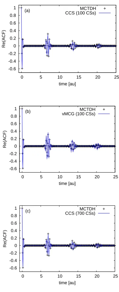
Fig. 4 Real part of the autocorrelation function for 6D Henon-Heiles problem. CCS and vMCG with

the basis of 100 CSs (frames a and b). CCS with the basis of 700 CSs and therefore with the same

amount of variational parameters (lower frame c). The results are compared with those of MCTDH

method (crosses).

-0.6 -0.4 -0.2 0 0.2 0.4 0.6 0.8 1

0 5 10 15 20 25

R

e

(A

C

F

)

time [au]

(a) MCTDH

CCS (100 CSs)

-0.6 -0.4 -0.2 0 0.2 0.4 0.6 0.8 1

0 5 10 15 20 25

R

e

(A

C

F

)

time [au]

(b) MCTDH

vMCG (100 CSs)

-0.6 -0.4 -0.2 0 0.2 0.4 0.6 0.8 1

0 5 10 15 20 25

R

e

(A

C

F

)

time [au]

(c) MCTDH

21

Fig. 5 Real part of the autocorrelation function for 10D Henon-Heiles problem with CCS with the

basis of 100 CSs (solid line) compared with results from MCTDH (crosses) (frame a) and the first

recurrence (frame b)

Fig. 6 Real part of the autocorrelation function for 10D Henon-Heiles problem with CCS with the

basis of 1000 CSs (solid line) compared with results from MCTDH (crosses) (frame a) and the first

recurrence (frame b)

-1 -0.5 0 0.5

0 2 4 6 8 10 12 14

R e (A C F ) time [au] (a)

CCS (100 CSs)

-0.15 -0.1 -0.05 0 0.05 0.1 0.15

5.5 6 6.5 7 7.5 8 8.5 9

R e (A C F ) time [au] (b) CCS (100) -1 -0.5 0 0.5 1

0 2 4 6 8 10 12 14

R e (A C F ) time [au] (a) MCTDH

CCS (1000 CSs)

-0.15 -0.1 -0.05 0 0.05 0.1 0.15

5.5 6 6.5 7 7.5 8 8.5 9

22

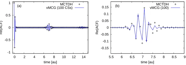
Fig. 7 Real part of the autocorrelation function for 10D Henon-Heiles problem with vMCG with the

basis of 100 CSs (solid line) compared with results from MCTDH (crosses) (frame a) and the first

recurrence (frame b)

Fig. 8 Comparison of the second recurrence of the autocorrelation function for 10D Henon-Heiles

problem obtained with CCS (1000 CSs) and vMCG (100 CSs) (frame a and b). Results from MCTDH

are shown by crosses.

-1 -0.5 0 0.5 1

0 2 4 6 8 10 12 14

R e (A C F ) time [au] (a) MCTDH

vMCG (100 CSs)

-0.15 -0.1 -0.05 0 0.05 0.1 0.15

5.5 6 6.5 7 7.5 8 8.5 9

R e (A C F ) time [au] (b) MCTDH vMCG (100) -0.04 -0.02 0 0.02 0.04

12 12.5 13 13.5 14 14.5 15 15.5 16

R e (A C F ) time [au] (a) MCTDH CCS (1000) -0.04 -0.02 0 0.02 0.04

12 12.5 13 13.5 14 14.5 15 15.5 16

23

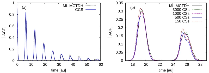
Fig. 9 Absolute value of the autocorrelation function for 18D Henon-Heiles problem with CCS

(3000CSs) and its convergence (frame a and b). Results from ML-MCTDH are shown by dashed line

on frame (a).

Fig. 10 Absolute value of the autocorrelation function for 18D Henon-Heiles problem with vMCG

(150CSs) and its convergence (frame a and b). Results from ML-MCTDH are shown by dashed line on

frame (a). 0 0.2 0.4 0.6 0.8 1

0 10 20 30 40 50 60

½ A C F ½ time [au] (a) ML-MCTDH CCS 0 0.05 0.1 0.15 0.2 0.25 0.3 0.35

18 20 22 24 26 28

½ A C F ½ time [au] (b) ML-MCTDH 3000 CSs 1000 CSs 500 CSs 150 CSs 0 0.2 0.4 0.6 0.8 1

0 10 20 30 40 50 60

½ A C F ½ time [au] (a) ML-MCTDH vMCG 0 0.05 0.1 0.15 0.2 0.25 0.3 0.35

18 20 22 24 26 28

24

Fig. 11 Absolute value of the autocorrelation function for 18D Henon-Heiles problem of strong

coupling, with CCS (4000 CSs) (frame a) and with vMCG (200 CSs) (frame b). Results from

ML-MCTDH are shown by dashed line on both frames.

Fig. 12 Absolute value of the autocorrelation function for 1458D Henon-Heiles problem (System 1)

with CCS (500CSs) (frame a and b). Results from ML-MCTDH are shown by dashed lines on both

frames. 0 0.05 0.1 0.15 0.2 0.25 0.3 0.35 0.4

0 10 20 30 40 50 60

½ A C F ½ time [au] (a) ML-MCTDH CCS 0 0.05 0.1 0.15 0.2 0.25 0.3 0.35 0.4

0 10 20 30 40 50 60

½ A C F ½ time [au] (b) ML-MCTDH vMCG 0 0.2 0.4 0.6 0.8 1

0 5 10 15 20

½ A C F ½ time [au] (a) ML-MCTDH CCS 0 0.1 0.2 0.3 0.4 0.5

25 30 35 40 45 50 55 60

25

Fig. 13 Absolute value of the autocorrelation function for 1458D Henon-Heiles problem (System 2)

with CCS (500CSs) (frame a and b). Results from ML-MCTDH are shown by dashed lines on both

frames. The difference between CCS and ML-MCTDH autocorrelation function for the System 2 is

less then the difference between ML-MCTDH results for System 1 and System 2

Fig. 14 Comparison of absolute value of the autocorrelation function for 1458D Henon-Heiles

problem. The CCS autocorrelation functions for System 1 and System 2 shown at the frame (a)

coinside. The ML-MCTDH results for the two systems are shown at the frame (b).

0 0.2 0.4 0.6 0.8 1

0 5 10 15 20

½ A C F ½ time [au] (a) ML-MCTDH CCS 0 0.1 0.2 0.3 0.4 0.5

25 30 35 40 45 50 55 60

½ A C F ½ time [au] (b) ML-MCTDH CCS 0 0.2 0.4 0.6 0.8 1

0 10 20 30 40 50 60

½ A C F ½ time [au]

(a) System 1

System 2 0 0.2 0.4 0.6 0.8 1

0 10 20 30 40 50 60

½ A C F ½ time [au]

(b) System 1

26

Tables

number of initial basis-vectors

deviation from MCTDH

1st recurrence

deviation from MCTDH 2nd recurrence

running time [sec]

compression [n=0.9905]

remaining basis-vectors

number of

variational parameters (number of remaining parameters are in brackets)

25 0.9495 0.2857 1.7 4.16 10 25 (10)

500 0.3752 0.2213 730.5 1.73 195 500 (195)

1000 0.3062 0.1519 2965.8 1.55 425 1000 (425)

Table 1. Deviation of the CCS result from that of MCTDH for a different number of initial

basis-vectors

number of initial basis-vectors

deviation from MCTDH

1st recurrence

deviation from MCTDH 2nd recurrence

running time [sec]

Compression [n=0.9905]

remaining basis-vectors

number of

variational parameters (number of remaining parameters are in brackets)

10 1.0586 0.2419 0.4 7.055 1 111 (11)

50 0.5252 0.2650 24.7 3.24 20 550 (220)

100 0.2536 0.1639 138.7 2.65 35 1100 (385)

Table 2. Comparison of the vMCG result with that of MCTDH for a different number of initial