Eddy Current Detection Methods for Surface Breaking Tight Cracks

INTRODUCTION

Norio Nakagawa

Center for NDE and Ames Laboratory Iowa State University

Ames, IA 50011

The eddy-current (EC) NDE method has been in use for quite some time, and efforts have been made to make it a fully quantitative method. To evaluate impedance signals for a given EC inspection system, one has to characterize the system as a whole, including both probes and

specimens. In particular, until probes are characterized, the

electromagnetic fields cannot be calculated . Naturally, the amount of numerical computation becomes a serious issue during the course of development. It is necessary to choose probes carefully so as to maximize the flaw-characterization capability, while keeping numerical

tasks within a reasonable size. Probes that are suitable for

quantitative assessment are presumably different in nature from those with maximum detection capability. Among all kinds of existing probes , the simplest characterizable probe is the uniform-field-eddy -current (UFEC) probe. In fact, a series of studies, both theoretical and experimental, were devoted to demonstrating potential capabilities of UFEC probes [1-9]. The present theoretical work is another entry in this series. The numerical procedure developed in this work is limited to the case where cracks are tightly closed. The procedure is

nevertheless capable, in principle, of dealing with an arbitrar y range of frequencies. In particular, it gives new theoretical pr edictions for impedance signals in the important frequency range where the skin depth becomes comparable with the size of cracks.

DESCRIPTION OF THE MODEL

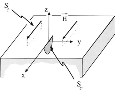
The system to be studied is illustrated schematically in Fig . 1. A metal specimen with a flat surface occupies the lower half-space. We consider a situation where there is a surface-breaking crack (denoted by S,) on the flat metal surface S1 • The crack is then scanned by a UFEC probe, which gives a uniform magnetic field distribution

H

paralle l to the flaw. For the reasons to be described below, the f law in this study is restricted to be a flat, tightly closed crack containing no asperity contacts. Otherwise, the crack faceS , can have an arbitrary shape. THEORETICAL FORMULATION

We will next briefly describe the mathematical methods. For the model given above, we shall first obtain electromagnetic field configurations by solving Maxwell's equations . One of t he s tandard approaches is to use the boundary-integral-equation (BIE) method [1,6 ]. As has been discussed, the advantage of this met hod over the

three-dimensional (3D) finite element method is that the BIE me thod requires many fewer unknown variables (in this case, the fields on the boundary surfaces) to be dealt with. This reduction in the number of

s

_c

Fig. 1. The eddy-current inspection system studied : A UFEC probe scans over a flat surface Sf of a metal specimen occupying the half space, giving a uniform magnetic field over the surface. The smaller surface denoted by Sc represents the face of a

surface-breaking tight crack.

unknown variables helps to minimize the amount of numerical computation. We also use the quasi-static approximation as usual, which further simplifies the matter.

Restricting the flaw to be a tightly closed crack reduces

computational tasks even further. It should be recalled that, when the crack is tight, one can use the potential method introduced by Bowler

[10]. Let us regard a tight crack as a limit of an open crack where the two .sides approach each other, but remain separated by an infinitesimal distance. Let Sc be the single limiting surface of the two approaching surfaces. Generally speaking, when applying the BIE method to this type of situation, one must be very careful in dealing with any possible singularity of the fields caused by the infinitesimal distance between the two surfaces,_ Here, we will exploit the situation, following Bowler. Let discH denote the discontinuity (or the jump) of the magnetic field

H

across Sc. It turns out that not all the field variables on the crack surface remain independent. Instead, only a single scalar function (denoted by <!>) defined on Sc remains an

independent surface variable. In terms of 4>, the discontinuitie s of the electromagnetic fields across Sc can be written as

discH-0, discE,--'f:J,~. (I)

Here, the first relation is deduced from a consideration over

microscopic physics, while the second equation is derived from the first and from Maxwell's equations. It should be emphasized that these

relations are valid only on the crack face Sc. This last reduction in the number of independent degrees of freedom makes the tight-crack problem especially tractable.

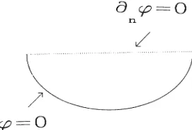
When adapting Bowler ' s method, we make a change in the boundary conditions imposed on the potential 4>. In his work, Bowler studied a subsurface crack, and showed that the potential takes a constant value along the edge of the crack, which can be set to vanish by definition . The same holds on the bottom edge of our surface -breaking crack. At the mouth of the crack , however, the boundary condition must be modified . For finding the correct condition, t he fluid-flow analogy is usef ul [1] . When eddy-current flow is regarded as fluid flow, the mouth region of the crack becomes the "stagnation point" at which the flow velocity vanishes. From this consideration, we conclude that the normal

[image:2.505.165.349.41.185.2]

a so=o

_n

\.

Fig. 2. The boundary conditions satisfied by the Bowler potential. It vanishes on the bottom edge of the crack, while, at the mouth of the crack, its normal derivative should vanish instead.

From a detailed study of the BIEs, a set of integral equations is derived to evaluate ~. _{More explicitly, it turns out that} ~satisfies a two-dimensional Poisson equation on S"

with a source term~. Starting from a Green's formula written forE> inside the metal, we first derive an integral equation for ~.

E~

0

_>(x,O,z)

-

J

dx'dz'G(x,z;x',z')~(x',z ' ),

Sc

(2)

(3)

where o£~0_{> is the eddy current density in the absence of the flaw, and}

where

G(x,z;x',z') (4)

Then, from (2) and the boundary conditions, we derive another BIE for a normal derivative of ~.

~co>(x,

z) = -

h

dsg(x, z;x(s),

z(s))o.~(s),

(S)

where C is a contour representing the bottom edge, and where

~<

0

_>=

J

_g~.

_{g(x, z;x'. z')= -(114n)Jn{(x-x')}2_{+ (z-z ' / } + (z' -1 - z ') . (6)}

These equations (3) and (5) can be solved numerically to find ~. Once it is obtained, then the impedance signal can be evaluated via

NUMERICAL RESULTS

[image:3.505.187.325.43.137.2]

1000 100

Q)

"'0 10

:J

....

c

Ol

0

~ 0.1

c

A

0.01

0.0014---~---r----~~----~

30 50 70 90 110

Phase [degrees]

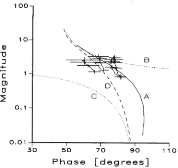
Fig. 3. The impedance signals due to a semi-elliptical tight crack of an aspect ratio 3 to 1. The curve A is the new result . The curves B and C are the results of the approximate theories, valid at either high or low frequencies . The curve A

interpolates Band C correctly. Moreover, it agrees with the several experimental data in the intermediate region. (See the text for references.)

there exists a set of experimental data in this particular region, which are also plotted in Fig. 3 [7]. Evidently, the present result agrees with the data better than the others do.

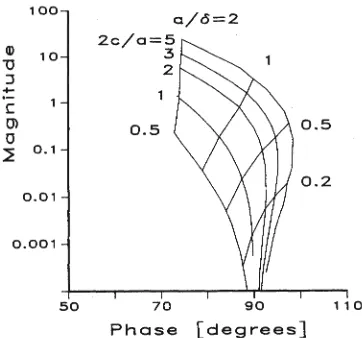
Second, we will present our approach toward solving inverse problems. Here, we use a model-based approach. Namely, we repeat similar calculations for cracks of various aspect ratios at various frequencies, and plot the results together to form a so -called

McFetridge chart (Fig. 4) [11]. When a measurement is made, one can get

c

Ol

0

100 10

~ 0 . 1 0 . 01 0.001

50

a/o = 2

2c/a=5

3

2

0.5

70 90

0 . 5

0.2

Phase [degrees]

110

[image:4.505.166.345.45.213.2] [image:4.505.164.345.435.604.2]

comparing the data with the chart. The particular chart provided in Fig. 4 is for semi-elliptical cracks with no internal contacts. Charts for other types of cracks could be obtained similarly.

Third, we will compare the current three-dimensional (3D) result with earlier 2D-model calculations. The motivation for this comparison is to examine the origin of surprisingly good agreement between 2D theory and 3D measurements observed earlier [8,9]. In Fig. 5, all the curves in Fig. 3 are reproduced except that the magnitudes are

normalized to unit crack length. We then overlay the 2D result (the curve D) in this plot, which is an impedance signal due to an infinitely long crack. Its depth is chosen to be equal to the average depth of the 3-to-1 semi-elliptical crack. The comparison shows how accurately the 2D theory can simulate the true 3D results. It is clear that the experimental data are in excellent agreement with the 3D predictions, although 2D theory works reasonably well within the currently achieved experimental accuracy.

TOWARD FURTHER APPLICATIONS

One may think that the NDE system described here is too restricted to be useful for realistic inspection problems. There are, however, many situations where one can regard field distributions as being locally uniform. Moreover, some of the restrictions are imposed merely for simplicity, and can be removed easily. In fact, the method can be generalized so that it is applicable to a wide variety of other EC inspection problems. It is impossible to mention all the possibilities here, except for a few immediate generalizations: (1) A mathematical formulation has been established for systems including more generally characterizable probes such as air-core coils. The software

implementation of this formulation is in order. (2) A study of tightly closed cracks cannot be complete unless one is able to deal with

contacting asperities. In fact, this problem was examined earlier in the framework of 2D models [8,9). It can be seen that the method reported here provides us with a means suitable for solving the problem in the 3D case. The contact problem, therefore, will be pursued in the near future as another immediate generalization of the present work.

(3) The limitation on specimen shapes should be relaxed for practical applications. There seems no fundamental obstacle in doing so except that the computational task will become more demanding. This is more of an engineering problem, challenging but straightforward. (4) These

100

I.

10 \ ·. \_.

Q)

"0

J B

...

c

Ol 0

~ A

0.1

0.011---~---r---T---~

30 50 70 90 110

Phase [degrees]

Fig. 5. Comparison between the 2D and 3D results. The curve D is an impedance curve due to an infinitely long crack . The other curves are reproductions of those in Fig. 3 except for the normalization. (See the text for details.)

[image:5.505.74.431.245.625.2] [image:5.505.163.343.436.606.2]

developments in forward calculations should open up new possibilities in other related studies such as inverse problems and probability-of-detectio~ modeling. Several initial studies in these directions have been started already, and more extensive progress can be expected in the near future.

ACKNOWLEDGMENTS

The author wishes to thank J. C. Moulder and J. Rose for

discussions. This work was supported in part by the Center for NDE at Iowa State University and in part by the Air Force Wright Aeronautical Laboratories/Material Laboratory, and performed at the Ames Laboratory, USDOE. Ames Laboratory is operated for the U.S. Department of Energy by Iowa State University under Contract No. W-7405-ENG-82.

REFERENCES

1. A. H. Kahn, R. Spal, and A. Feldman, J. Appl. Phys. 48, 4454 (1977); A. H. Kahn, in Review of Progress in Quantitative NDE, edited by D. 0. Thompson and D. E. Chimenti (Plenum Press, New York, 1982), Vol. 1, pp. 369-373.

2. B. A. Auld, "Theoretical Characterization and Comparison of Resonant-Probe Microwave Eddy-Current Testing with Conventional Low-Frequency Eddy-Current Methods," in Eddy Current

Characterization of Materials and Structures, ASTM STP 722, G. Birnbaum and G. Free, eds., American Society for Testing and Materials, Philadelphia (1981).

3. T. G. Kincaid, in Review of Progress in Quantitative NDE, edited by D. 0. Thompson and D. E. Chimenti (Plenum Press, New York, 1982), Vol. 1, pp. 355-356 .

4. W. D. Dover, F. D. W. Charlesworth, K. A. Taylor, R. Collins, and D. H. Michael, in The Measurement of Crack Length and Shape during Fatigue and Fracture, C. J. Beevers, ed., EMAS, Warley (1980); W. D. Dover, F. D. W. Charlesworth, K. A. Taylor, R. Collins, and D. H. Michael, in Eddy Current Characterization of Materials and Structures, ASTM STP 722, G. Birnbaum and G. Free, eds., American Society for Testing and Materials, Philadelphia (1981).

5. B. A. Auld, F. G. Muennemann, and D. K. Winslow, J . Nondestr. Eval .

z,

1 (1982); B. A. Auld, F. G. Muennemann, and M. Riaziat,

"Quantitative Modeling of Flaw Responses in Eddy Current Testing," in Research Techniques in Nondestructive testing, Vol. 7, R.S. Sharpe, ed., Academic Press, London (1984) .

6. V. G. Kogan, G. Bozzolo, and N. Nakagawa, in Review of Progress in Quantitative NDE, edited by D. 0 . Thompson and D. E. Chimenti

(Plenum Press, New York, 1987), Vol. 6A, pp. 153-160.

7.' J. C. Moulder, P. J. Shull, and T. E. Capobianco, in Review of Progress in Quantitative NDE, edited by D. 0. Thompson and D. E. Chimenti (Plenum Press, NewYork, 1987), Vol. 6A, pp. 601-610. 8. J. C. Moulder, N. Nakagawa, and

P.

J. Shull , in Review of Progress

in Quantitative NDE, edited by D. 0. Thompson and D. E. Chimenti (Plenum Press , New York, 1988), Vol . 7A, pp. 147-155.

9. N. Nakagawa, V. G. Kogan, and G. Bozzolo, in Review of Progress in Quantitative NDE, edited by D. 0. Thompson and D. E. Chimenti

(Plenum Press, New York, 1988), Vol . 7A, pp . 173-179.

10. J. R. Bowler, in Review of Progress in Quantitative NDE , edited by D. 0. Thompson and D. E. Chimenti (Plenum Press, New York, 1986), Vol. SA, pp. 149-155.