This is a repository copy of
Finite impulse response filter design using a forward
orthogonal least squares algorithm
.
White Rose Research Online URL for this paper:
http://eprints.whiterose.ac.uk/74505/
Monograph:
Wu, X., Lang, Z.Q. and Billings, S.A. (2005) Finite impulse response filter design using a
forward orthogonal least squares algorithm. Research Report. ACSE Research Report
no.904 . Automatic Control and Systems Engineering, University of Sheffield
[email protected] https://eprints.whiterose.ac.uk/ Reuse
Unless indicated otherwise, fulltext items are protected by copyright with all rights reserved. The copyright exception in section 29 of the Copyright, Designs and Patents Act 1988 allows the making of a single copy solely for the purpose of non-commercial research or private study within the limits of fair dealing. The publisher or other rights-holder may allow further reproduction and re-use of this version - refer to the White Rose Research Online record for this item. Where records identify the publisher as the copyright holder, users can verify any specific terms of use on the publisher’s website.
Takedown
If you consider content in White Rose Research Online to be in breach of UK law, please notify us by
Finite Impulse Response Filter Design Using A
Forward Orthogonal Least Squares Algorithm
Xiaofeng Wu, Z Q Lang and S.A.Billings
Department of Automatic Control and Systems EngineeringThe University of Sheffield Sheffield, S1 3JD, UK Email: [email protected]
Abstract— This paper is concerned with the application of
forward Orthogonal Least Squares (OLS) algorithm to the design of Finite Impulse Response (FIR) filters. The focus of this study is a new FIR filter design procedure and to compare this with traditional methods known as the fir2() routine, provided by MATLAB.
Keywords–Orthogonal Least Squares; Finite Impulse Response Filter; Parameter Estimation; Structure Selection
I. INTRODUCTION
Linear Finite Impulse Response (FIR) filter coefficients design has been extensively studied. Classical methods involve designing a FIR filter based on Fourier Series theory and Inverse-DFT transform. This is also the primary principle of the FIR design in MATLAB. However, researchers still continue to study improved methods for FIR filter design. Lertniphonphun developed an algorithm which designs a FIR filter using a weighted Chebyshev norm based optimization approach [1]. FIR designs subject to upper and lower bounds on the frequency response magnitude were studied by Wu [2]. Yong [3] investigated the design of FIR filters using a cluster of workstations as computing platform. Given the benefits of FIR filter applications to the digital signal processing field, it is reasonable to believe the feasibility of further innovation in this specific area.
There are many well developed FIR filter design methods. The fir2() routine is one method embedded in the MAT-LAB signal processing toolbox, which can be used to design frequency sampling-based FIR filters with arbitrarily shaped frequency responses. In the present study, fir2() is used as a representative of traditional FIR filter design and is compared with a new design method based on the forward orthogonal least squares algorithm.
The Orthogonal Least Squares (OLS) algorithm was derived as an effective solution for structure selection and parameter estimation in nonlinear system identification [4]. In this paper, a new OLS based procedure is introduced to provide an alter-native method for FIR filter design. The new method employs the OLS algorithm to determine the terms and parameters of a FIR filter in order to meet a specified frequency response requirement. Compared with the traditional fir2() procedure, the new method not only provides a different way of designing FIR filters but also offers several advantages. More impor-tantly, the OLS based design can easily be extended to deal
with nonlinear filter designs which are issues currently under study and will be discussed in a future publication.
The paper is organized as follows. First, the fir2() routine and associated theory are introduced. Then, the new OLS based FIR design is proposed, and a comparison of the new method with the fir2() routine is conducted to show the advantages and potential of the new approach. Finally, results of case studies are presented and discussed in detail.
II. THE FIR2() ROUTINE FORFIR FILTERDESIGN
Let H(ejω) denote the frequency response of the digital
transfer function H(z) to be designed to approximate the desired (ideal) response Hd(ejω). The basic idea behind
the fir2() routine in MATLAB is to determine the transfer function coefficients so that the difference between H(ejω)
and Hd(ejω) for all values of ω in the range 0 ≤ ω ≤ π
is minimized. The MATLAB routine fir2() satisfies the least-square criterion [6].
BecauseHd(ejω)is a periodic function, it can be expressed
as a Fourier series:
Hd(ejω) =
∞ X
n=−∞ hd[n]e
−jnω (1)
with Fourier coefficients given by
hd[n] = 1
2π Z π
−π
Hd(ejω)ejnωdω − ∞< n <∞ (2)
The fir2() routine is a frequency sampling approach. The desired frequency responseHd(ejω)is first uniformly sampled
atN equally spaced pointsωk = 2πk/N, k= 0,1, ..., N−1,
providing N frequency samples. These samples compose of anN-point DFTH[k]whoseN-point inverse-DFT yields the impulse response coefficients h[n]of the FIR filter of length N. From equation (1),
H[k] =Hd(ejωk) =Hd(ej(2πk/N)) =
∞ X
l=−∞
hd[l]WNkl (3)
whereWN =e−j(2π/N). An inverse-DFT ofH[k] yields
h[n] = 1
N
N−1 X
k=0
H[k]W−kn
The coefficientsh[n]often produce an oscillatory magnitude response which is called Gibbs phenomenon. In order to reduce the ripples, a window function is finally used to yield the filter coefficients.
The MATLAB syntax formulation
b=f ir2(N, f, m) (5)
designs a N-th order FIR filter and returns the filter coeffi-cients in vector b of length N+ 1. Vectorsf andm specify the frequency and corresponding magnitude sample points respectively. In practice, f is the normalized frequency point vector ranging from 0 to 1, where 1 represents the Nyquist frequency (corresponding to half the sample rate). m is a vector containing the desired magnitude response at the points specified in f. By default, fir2() uses a Hamming window. Usually, b is real, symmetric. Without loss of generality, It is assumed that even symmetric coefficients obey b[k] =
b[N+ 2−k], k= 1,2, ..., N+ 1 [7].
III. THEORTHOGONALLEASTSQUARESALGORITHM
Model identification can generally be formulated as a standard least squares problem. Compared with simple least squares algorithms, the orthogonal least squares method has been demonstrated to be a powerful means to achieve this objective. Basically, the orthogonal algorithm was developed as an approach to combine parameter estimation and model structure detection. The principal idea of the algorithm is to decouple the candidate terms by introducing an orthogonal transform so that selected terms will not be affected when a new term is selected. For most system representations, the orthogonal decomposition approach of the regressor matrix avoids possible ill-conditioning and presents more accurate results. The forward OLS algorithm is based on the classical Gram-Schmidt method [4] [5].
A. Parameter Estimation
Consider a linear regression model
y(k) =
n
X
i=1
φi(k)θi+e(k) k= 1, ..., N (6)
where y(k) represents the k-th measurement, N is the data length, n is the number of column vectors, φi(k) and θi
denote the regressors and parameters respectively, and e(k)
is the modelling error, assumed to be a zero mean white noise sequence. Using the orthogonal algorithm, the parameters θi
are estimated by transforming model (6) into an equivalent auxiliary model
y(k) =
n
X
i=1
giwi(k) +e(k) (7)
where wi(k) are constructed to be orthogonal and gi are
constant coefficients.
First, orthogonal vectors can be constructed over the given data record as
w1(k) =φ1(k) (8)
wj(k) =φj(k)− j−1 X
i=1
αijwi(k) (9)
where
αij =
PN
k=1wi(k)φj(k) PN
k=1wi2(k)
½
j= 1, ..., n
i= 1, ..., j−1, j (10)
and from the orthogonal property, there is
wi(k)wj(k) = 0 i6=j (11)
where the overline denotes the time average over the data length.
The second step consists of estimating the coefficients gi,
which is given by
ˆ
gi=
PN
k=1wi(k)y(k)
PN
k=1w2i(k)
(12)
Finally, the unknown system parameters can be calculated fromgˆi according to
ˆ
θn= ˆgn (13)
ˆ
θi= ˆgi− n
X
j=i+1
αijθˆj i=n−1, n−2, ...,1 (14)
The auxiliary regressor wi(k) are orthogonal so that
ad-ditional terms can be added to the model without the need to recompute all the previous ˆgj, j < i. The orthogonal
least squares parameter estimation algorithm is therefore very simple and easy to implement.
B. Structure Selection
The determination of a parsimonious representation of a sys-tem is one of the most important tasks in syssys-tem identification. A great advantage of the orthogonal estimator is the possibility of selecting the relevant terms using the Error Reduction Ratio (ERR). The basic principle is given below.
Multiplying equation (7) by itself gives
y2(k) =
n
X
i=1 g2
iw2i(k) +e2(k) (15)
The above equation shows that the contribution of each term g2
iw2i(k)to the output energyy2(k). Expressing this quantity
as a fraction of i-th term as
ERRi=
ˆ
g2
iw2i(k)
y2(k) =
ˆ
g2
i
PN
k=1wi2(k)
PN
k=1y2(k)
×100% 1≤i≤n
(16) The forward regression procedure is implemented as: 1) Consider all regressorsφi(k) i= 1,2, ..., nas possible
2) Consider all the φi(k) i= 1,2, ..., n, i6=j as possible
candidates forω2(k)calculating through equation (9), (12) and (16), find the maximum of ERR2 for example ERR(2l) = max{ERR(2i),1 ≤ i ≤ n, i 6= j}. Then the second term selected should be thelth term. i.e.ω2(k) =φl(k)−α12ωl(k).
3) Continue the process and in each loop, the term with the maximum error reduction ratio is then selected to produce the term ωi(k).
The ERR value could be computed together with the pa-rameter estimate to indicate the significance of each candidate term. Insignificant terms will be discarded from the model by defining threshold value of ERR summation. The forward Orthogonal Least Squares algorithm is terminated when the summation of ERR values is close to 100%.
IV. OLS-BASEDFIR FILTERDESIGN
In the following, the FIR filter design is formulated as a difference equation with2N+ 1coefficients [8],
y(n) =
N
X
i=−N
bix(n−i) (17)
Applying theztransform to both sides of equation (17) yields
H(z) = Y(z)
X(z) =
N
X
i=−N
biz
−i (18)
Replacing z in equation (18) with ejω yields the filter fre-quency response
H(ejω) =
N
X
n=−N
bne−jnω (19)
Since the filter coefficients can only be real valued, the fre-quency response must be conjugate symmetric. This premise is the same as for the fir2() routine in MATLAB. From equation (19), a noncausal filter is designed. Then by shifting the filter coefficients, the filter can be made to be causal and practical. A causal FIR filter with impulse response bc[n] can be
derived from b[n] by shifting the sequence by N samples. i.e.
bc[n] =b[n−N] (20)
Accordingly the corresponding transfer function is
H(z) =
2N
X
i=0
bc[i]z−i (21)
The key step in using the OLS algorithm to design the FIR filter coefficients θi involves the choice of arguments,
φi and y(k) in equation (6). Comparing equation (6) and
(19), it can be concluded that the regressor φi corresponds
to each frequency component e−jnω, y(k) corresponds to
H(ejω), and the index k in equation (6) should be replaced
by frequency sampling points ω in equation (19). Using all these relationships, the filter coefficients {bn} can be easily
determined using the forward OLS algorithm.
The matrix expression of system parameter estimation on equation (6) is
Y = ΦΘ + Ξ (22)
Consequently, the related FIR filter design is of the form
H =U β+ Ξ (23)
where H, a (2m+ 1)×1 vector, represents the frequency response at the equally divided frequency sampling points as
H =
H(ejω−m) .. . H(ejωm)
(24)
andU, a(2m+ 1)×(2N+ 1)complex matrix, is given by
U =
e−j(−N)ω−m . . . e−j(N)ω−m ..
. . .. ...
e−j(−N)ωm . . . e−j(N)ωm
(25)
In order to apply the OLS algorithm to perform FIR filter design, equation (23) is partitioned into real and imaginary parts to yield
[HR
HI
] = [UR
UI
]β+ [ΞR ΞI
] (26)
where the subscriptRdenotes the real part andIthe imaginary part [9].
The OLS algorithm is employed to compute the parameters in the column vectorβ, a(2N+ 1)×1coefficients vector,
β=
b−N
.. . bN
(27)
which are the FIR filter coefficients.
V. CASESTUDY ANDDISCUSSIONS
In order to verify the OLS approach to FIR filter design and compare the OLS-based approach with the fir2() routine in MATLAB, a lowpass FIR filter design is considered in this section.
A. Lowpass FIR Filter Designs
Consider an order-N (N=10) lowpass FIR filter that has frequency response defined as normalized frequency f =
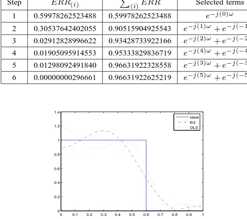
{0,0.6,0.6,1} and magnitude responsem={1,1,0,0}, The duplicated frequency points at f = 0.6 indicates a step in frequency response. The desired frequency response is depicted in Figure 1.
The ideal frequency response can be analytically described as
Hd(ω) =
½
1 |ω| ≤0.6π
0 0.6π≤ |ω| ≤π (28)
The impulse response corresponding to the frequency response is given by
hd(n) =
0.6π π
sin 0.6πn
0 0.1 0.2 0.3 0.4 0.5 0.6 0.7 0.8 0.9 1 0
0.2 0.4 0.6 0.8 1 1.2
[image:5.612.313.563.100.248.2]Ideal (Desired) Lowpass Filter Frequency Response
Fig. 1. Desired Normalized Frequency Response
which are the components of the Fourier Series. Based on these coefficients, the following discussion focuses on a comparison between the filter design methods.
First, the fir2() routine, which involves applying equation (5) in MATLAB, is used to design the FIR filter coefficients with orderN = 10, andf andmas given above. The design results without applying windowing are shown in the column under bf ir2(n)in Table I.
Then the OLS based approach is applied for the design with the following considerations:
1) Hd(ejω) are equally sampled over [−π, π] with a
sam-pling interval of 1000π to produce the sampled frequency vector ω = [ω−m, . . . , ωm] and the desired frequency response over
the sampled frequenciesH = [H(e−jω−m), . . . , H(e−jωm)]τ.
2) Assume that the filter coefficients are symmetric, i.e. b−i = bi, 0 ≤ i ≤ N. Therefore, only half the coefficients
β1, the(N+ 1)×1 column vector
β1=
b−N
.. .
0
(30)
need to be determined and matrix U in equation (25) can consequently be reduced to
U1=
(e−j(−N)ω−m+e−j(N)ω−m) . . . e−j(0)ω−m ..
. . .. ...
(e−j(−N)ωm+e−j(N)ωm) . . . e−j(0)ωm
(31) The design results (again without applying windowing) are shown in the column under bOLS(n)in Table I.
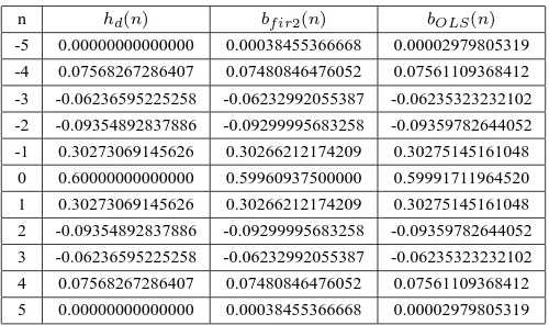
3) Using the forward OLS algorithm based on equa-tion (26), the term selecequa-tion stopped when PERR10 =
0.96631922625219and altogether 10 terms were included in FIR filter.
B. Algorithm Analysis
From Table I, it can be observed that the difference between the two design methods is not significant at all, but the OLS based design is slightly better than the design using the fir2() routine. Two aspects of analysis are conducted in the following for the two different design methods.
TABLE I
COEFFICIENTSCOMPARISON OF THETWOALGORITHMS AND THEIDEAL FILTER.(ORDER-10)
n hd(n) bf ir2(n) bOLS(n) -5 0.00000000000000 0.00038455366668 0.00002979805319 -4 0.07568267286407 0.07480846476052 0.07561109368412 -3 -0.06236595225258 -0.06232992055387 -0.06235323232102 -2 -0.09354892837886 -0.09299995683258 -0.09359782644052 -1 0.30273069145626 0.30266212174209 0.30275145161048 0 0.60000000000000 0.59960937500000 0.59991711964520 1 0.30273069145626 0.30266212174209 0.30275145161048 2 -0.09354892837886 -0.09299995683258 -0.09359782644052 3 -0.06236595225258 -0.06232992055387 -0.06235323232102 4 0.07568267286407 0.07480846476052 0.07561109368412 5 0.00000000000000 0.00038455366668 0.00002979805319
1) Analysis of the Filter Coefficients: According to equa-tion (3) and (4),
h[n] = 1
N
N−1 X
k=0 ∞ X
l=−∞
hd[l]WNklW
−kn
N (32)
and the relation between the ideal filter Fourier series and the frequency sampling impulse response coefficients can be simplified by swapping the order of summation [6],
h[n] =
∞ X
m=−∞
hd(n+mN) 0≤n≤N−1 (33)
Equation (33) implies that h[n] from the fir2() routine is obtained from hd[n] by adding an infinite number of shifted
replicas of hd[n], with each replica shifted by an integer
multiple of N sampling instants. Since hd[n] is an infinite
length sequence according to equation (2), which shows that the coefficientsh[n]computed from the inverse-DFT can not be the same as the ideal result. This is the intrinsic shortcoming of the fir2() routine.
However, the OLS based method doesn’t possess this prob-lem. This explains the slightly better performance of the OLS algorithm compared to the fir2() routine.
Another point is that fir2() may miscalculate coefficients when a higher frequency resolution is used in the computation. Consider the case f = [0,0.6,0.6,1] and frequency interval as 1000π cases for the fir2() routine, the coefficients estimation through this approach is listed in Table II.
Considering next the frequency interval as 1000π and 10000π , the results for the OLS algorithm are given in Table III.
It is obvious that for the OLS method the higher the frequency resolution, the closer the results converge to the ideal result, and the better the effect of the design. While for the fir2() routine, the limitation is that for higher frequency resolution situations, it may perform worse.
TABLE II
COEFFICIENTSCOMPARISON OF FIR2()ANDIDEALONES.(ORDER-10)
n hd(n) f= [0,0.6,0.6,1] interval=1000π -5 0.00000000000000 0.00038455366668 0.00474422289254 -4 0.07568267286407 0.07480846476052 0.07381197433722 -3 -0.06236595225258 -0.06232992055387 -0.06603956659887 -2 -0.09354892837886 -0.09299995683258 -0.08955904050756 -1 0.30273069145626 0.30266212174209 0.30410856041926 0 0.60000000000000 0.59960937500000 0.59521484375000 1 0.30273069145626 0.30266212174209 0.30410856041926 2 -0.09354892837886 -0.09299995683258 -0.08955904050756 3 -0.06236595225258 -0.06232992055387 -0.06603956659887 4 0.07568267286407 0.07480846476052 0.07381197433722
5 0.00000000000000 0.00038455366668 0.00474422289254
TABLE III
COEFFICIENTSCOMPARISON OFOLSANDIDEALONES.(ORDER-10)
n hd(n) interval=1000π interval=10000π -5 0.00000000000000 0.00002979805319 0.00000353824178 -4 0.07568267286407 0.07561109368412 0.07567239400313
-3 -0.06236595225258 -0.06235323232102 -0.06236359287874 -2 -0.09354892837886 -0.09359782644052 -0.09354792546414 -1 0.30273069145626 0.30275145161048 0.30273168582088 0 0.60000000000000 0.59991711964520 0.59998368155733 1 0.30273069145626 0.30275145161048 0.30273168582088 2 -0.09354892837886 -0.09359782644052 -0.09354792546414 3 -0.06236595225258 -0.06235323232102 -0.06236359287874 4 0.07568267286407 0.07561109368412 0.07567239400313 5 0.00000000000000 0.00002979805319 0.00000353824178
ERR value, the number of terms in the desired FIR filter can be actively controlled to achieve a compromise between the filter complexity and the filter performance. This is another advantage of the OLS based method over the fir2() routine, which can do nothing on this point.
To demonstrate the merits, the term selection process of the OLS based design is illustrated in Table IV. Clearly, if the target value of PERR is only 95%, then the FIR filter of seven terms
HOLS(ejω) =b−4e
−j(−4)ω+b
−2e
−j(−2)ω+b
−1e −j(−1)ω
+b0e−j(0)ω+b1e−j(1)ω+b2e−j(−2)ω+b4e−j(4)(34)ω
is sufficient to satisfy the design requirements. After the fourth step, the summation of ERR reaches P
ERR =
0.95333829836719.
However, the seven terms FIR filter design using fir2() is
Hf ir2(ejω) =b−3e
−j(−3)ω+b
−2e
−j(−2)ω+b
−1e −j(−1)ω
+b0e−j(0)ω+b1e−j(1)ω+b2e−j(−2)ω+b3e−j(3)(35)ω
The difference is that the fir2() routine selects frequency component n= 3but notn= 4. Through further calculation,
TABLE IV
ERRVALUEANALYSIS FOREACHSTEP.(ORDER-10,FREQUENCY INTERVAL=1000π )
Step ERR(i) P(i)ERR Selected terms
1 0.59978262523488 0.59978262523488 e−j(0)ω
2 0.30537642402055 0.90515904925543 e−j(1)ω+e−j(−1)ω
3 0.02912828996622 0.93428733922166 e−j(2)ω+e−j(−2)ω
4 0.01905095914553 0.95333829836719 e−j(4)ω+e−j(−4)ω
5 0.01298092491840 0.96631922328558 e−j(3)ω+e−j(−3)ω
6 0.00000000296661 0.96631922625219 e−j(5)ω+e−j(−5)ω
0 0.1 0.2 0.3 0.4 0.5 0.6 0.7 0.8 0.9 1 0
0.2 0.4 0.6 0.8 1 1.2 1.4
[image:6.612.311.554.114.329.2]Ideal fir2 OLS
Fig. 2. Frequency Response Magnitudes with Term Selection (PERR= 0.95333829836719)
the value of ERR for term (e−j(3)ω + e−j(−3)ω) on the
fourth step is 0.01296523967681, which makes P ERR′
= 0.94725257889847, unqualified for the design requirement.
The comparison of design results and corresponding co-efficients are depicted respectively in Figure 2 and 3. The significance of frequency component n = 4 is greater than that ofn = 3, therefore, the OLS algorithm takes advantage and picks up the most significant term to improve the overall system design.
VI. CONCLUSIONS
In this paper, a new OLS based FIR filter design procedure has been proposed and compared with the traditional FIR filter design routine fir2() in MATLAB. Several advantages of the new method over traditional method have been demonstrated
1 2 3 4 5 6 7 8 9 10 11 −0.1
0 0.1 0.2 0.3 0.4 0.5 0.6
[image:6.612.361.512.590.696.2]Ideal fir2 OLS
using simple design examples. The simulation studies verify the effectiveness and value of this new approach. We are currently extending the OLS based method to deal with the issue of nonlinear filter designs. These results will be presented in a future publication.
ACKNOWLEDGMENT
XFW expresses his thanks to the department of ACSE, the University of Sheffield for support from a research scholarship. ZQL and SAB greatly acknowledge that part of this work was supported by Engineering and Physical Science Research Council, UK.
REFERENCES
[1] Lertniphonphun, W. & McClellan, J.H. [1998] Complex frequency response FIR filter design, Proceedings of the 1998 IEEE International Conference Vol. 3, pp. 1301-1304
[2] Wu, S.P. & Boyd, S. & Vandenberghe, L. [1997] FIR Filter Design via Spectral Factorization and Convex Optimization, Applied Computational Control, Signal and Communications pp. 1-33
[3] Yong C.L. & Sun, Y. & Ya J.Y. [2002] Design of discrete-coefficient FIR filters on loosely connected parallel machines, Signal Processing, IEEE Transactions Vol. 50, pp. 1409-1416
[4] Chen, S. & Billings, S.A. & Luo, W. [1989] Orthogonal Least Squares Methods and Their Application to Nonlinear System Identification, International Journal of Control 50(5):1873–1896, 1989.
[5] Lay, D.C. [1998] Linear Algebra and Its Applications, Second Edition, Addison-Wesley, pp. 378-402.
[6] Mitra, S.K. [1998] Digital Signal Processing A Computer Based Ap-proach, First Edition, McGraw-Hill, New York, pp. 462-468.
[7] Jackson, L.B. [1996] Digital Filters and Signal Processing, Third Edi-tion, Kluwer Academic Publishers, Boston, pp. 301-307.
[8] Mulgrew, B. & Grant, P. & Thompson, J. [1999] Digital Signal Process-ing Concepts & Applications, Palgrave, New York, pp. 150-154. [9] Swain, A.K. & Billings S.A. [1998] Weighted Complex Orthogonal