Experimental Observation of Flow Fields Around Active Janus Spheres

Andrew I. Campbell,1 _{Stephen J. Ebbens,}1,∗ _{Pierre Illien,}2, 3, 4 _{and Ramin Golestanian}2,† 1

Department of Chemical and Biological Engineering, University of Sheffield Mappin Street, Sheffield S1 3JD, UK

2

Rudolf Peierls Centre for Theoretical Physics, University of Oxford, Oxford OX1 3NP, UK 3

Max Planck Institute for the Physics of Complex Systems, Nothnitzer Str. 8, 01187 Dresden, Germany 4_{ESPCI Paris, UMR Gulliver, 10 Rue Vauquelin, 75005 Paris, France}

(Dated: February 14, 2018)

The hydrodynamic flow field around a catalytically active colloid is probed using particle tracking velocimetry both in the freely swimming state and when kept stationary with an external force. Our measurements provide information about the fluid velocity in the vicinity of the surface of the colloid, and confirm a mechanism for propulsion that was proposed recently. In addition to offering a unified understanding of the nonequilibrium interfacial transport processes at stake, our results open the way to a thorough description of the hydrodynamic interactions between such active particles and understanding their collective dynamics.

Introduction.— The ability to design active colloids and to accurately control their motion in a fluid envi-ronment is one of the cornerstones of modern physical sciences, and has motivated a significant amount of work over the past years [1–3]. In particular, it has enabled experimental efforts to mimic functions inspired by cel-lular biology, such as cargo transport or chemical sensing, which might lead to radically new medical applications. From a theoretical point of view, such objects do not obey the laws of equilibrium statistical physics, and the description of their non-equilibrium dynamics remains a major challenge. Understanding these non-equilibrium phenomena could help us develop a new paradigm in en-gineering by designing emergent behavior.

Phoretic transport has emerged as a prominent mech-anism for non-equilibrium activity. It has been known for many decades that the interactions between a par-ticle immersed in a fluid and an inhomogeneous field— which can be a chemical concentration, a temperature, and electrostatic potential—can lead to force-free and torque-free propulsion [4–6]. Although the field gradi-ents can be externally imposed on the phoretic particles, a most interesting situation arises when the particle gen-erates them itself. For instance, the particle can bear an “active site”, which degrades solute particles present in the bulk. The resulting asymmetric distribution of reaction products creates a nonzero slip velocity at the surface of the particle and yields self-propulsion [7, 8].

A number of different particles that break fore-aft sym-metry have been designed, including bimetallic rods [9] and insulator spheres with only one metal-coated hemi-sphere [10] that are able to decompose hydrogen perox-ide with Pt as a catalyst. It was shown that bimetal-lic swimmers are able to decompose fuel simultaneously at both ends. Such an electrochemical process results in an electron transfer across the object, and the

as-∗_{[email protected]}

†_{[email protected]}

sociated proton movement in the solution permits self-electrophoretic propulsion. However, despite extensive studies, the phoretic mechanisms at stake in Janus sphere propulsion are not yet well established, and have been the subject of recent debates. Although their constitu-tive material (typically polystyrene) is an insulator, re-cent experimental investigations have revealed that elec-trokinetic effects need to be taken into account together with diffusiophoretic effects to fully describe the propul-sion mechanism [11–14]. The emergence of such effects is permitted by the inhomogeneity of Pt coating, which is thicker at the pole of the colloid than at its equator. We recently proposed a mechanism where the motility of the Pt-PS sphere is linked to closed current loops, which start at the equator of the particle and end at its pole [Fig. 1(a)]. These conjectured closed proton loops are ex-pected to yield a strongly asymmetric slip velocity across the surface of the colloid [11, 14]. This proposal allowed us to explain the ionic strength sensitivity of the swim-ming velocity and the non-equilibrium surface alignment phenomenon observed in our experiments [15]. However, direct experimental evidence that proves this conjecture has been lacking so far.

Here, we measure the flow fields around moving Pt-PS Janus particles using Particle Tracking Velocimetry (PTV). This is particularly challenging due to the ran-dom stochastic Brownian re-orientation of the moving Pt-PS Janus particles. In a related study reporting the flow field around swimming microorganisms [16] photo-tactic guidance was used to prevent rotation. However, in absence of an equivalent mechanism for Pt-PS Janus par-ticles, here we developed pattern matching image analy-sis algorithms to allow tracer particle motion to be quan-tified relative to the frame of reference of a freely moving and rotating Pt-PS Janus particle. This method also allowed us to arrive at average flow fields derived from observations of many different Pt-PS Janus particles.

Experimental methods.— Our experimental system consisted of a 4 cm_×1 cm _× 0.1 cm glass cuvette filled with a very dilute suspension ofa= 3.5µm polystyrene Janus spheres in 10 wt% H2O2 solution [10]. The Janus

t P SP

ê êr ê

(a)

(b)

(c)

θ

θ

a

0 0.05 0.1 0.15 0.2 0.25

0 π/4 π/2 3π/4 π

v(

θ)

θ

(e)

(d) (f)

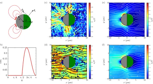
FIG. 1. (a) Sketch of the Pt-PS Janus particle and notations. ˆeis the direction of swimming. The red arrows represent the current loops that start at the equator of the particle and end at its pole [11, 14, 15]. (b) Plot of the slip velocityv(θ) that is used to compute analytically the flow field around the Janus particle, which is compared with the experimental observations. (c)-(f) Streamlines around the Janus particles obtained experimentally (left) and analytically (right), in the two situations where the particle is stuck (top) and freely moving (bottom). The background colors represent the magnitude of the velocity u=|u|rescaled by the swimming velocity of the Janus particle when it is freely moving.

spheres are coated on one hemisphere with a thin evap-orated layer of Pt metal with a maximum thickness of 10 nm. To the suspension we added 3µL of a 1.0 wt% dis-persion of green fluorescent polystyrene spheres (radius = 0.25µm) to act as tracer particles. After vigorous shak-ing to fully disperse the tracer particles the cuvette was placed on the stage of a Nikon Eclipse LV100 microscope fitted with a Nikon 20_×0.45 N.A. objective. Operating in fluorescence mode using the blue excitation band of a Nikon B2A filter cube the tracer particles at the top of the cuvette were brought into focus. After a few minutes equilibration time some of the gravitactic Janus sphere swimmer particles [17] had traveled to the top of the cu-vette and could be seen translating parallel to the glass surface. After a period some of the Janus spheres became stuck to the surface, probably due to impurities on the surface.

We recorded images (512 _× 512 pixels) of the Janus spheres moving through the field of tracer particles using an Andor Neo camera at a frequency of 100 Hz. We note that focussed at the top of the cuvette the bulk of the tracer particles are not in focus. This provided a background level of illumination that enabled us to image the non-fluorescent Janus spheres, where they appeared as a transparent disc with a shadow covering one half of the disc indicating the position and rotation of the Pt cap. Tracking of the tracer particles has been

described before [10, 18] but the Janus spheres required a different approach. We used the pattern matching functions of the LabView graphical programming lan-guage to obtain the center position of a Janus sphere and the angle of rotation of its Pt cap. Tracer particle and Janus sphere trajectories were smoothed to suppress Brownian noise. We then calculated the frame-by-frame vectors along the tracer particle trajectories relative to the position and angle of the Janus sphere. The vectors were then placed on a 0.5µm grid with the Janus sphere at the origin and an angle of rotation of 0o_{. Where multiple vectors occupied the same grid} position an average vector was calculated. About 120 s of video data of seven Janus spheres and 115 s of video data of four Janus spheres were used to generate the average flow field around the translating and stuck Janus spheres respectively. Figure 1 shows the experimentally determined flow fields around both stuck and trans-lating Janus spheres, with streamlines generated using the streamplot function of the Python Matplotlib library.

Theoretical description.— In the low Reynolds num-ber limit, the flow fielduaround the Janus colloid is the solution of the Stokes problem:

−η_∇2_u= −∇p,

[image:2.612.65.551.48.317.2]

with boundary conditions imposed by the phoretic mech-anisms taking place at the surface of the colloid.

In the situation where the Janus swimmer is stuck to the glass slide, the total flow field may be written as

u=uph+umono, whereuphis the phoretic contribution to the flow field andumono _{is the contribution from the} force monopole that maintains the colloid steady in the laboratory reference of frame. The phoretic contribution originates from a non-zero slip velocity at the surface of the colloid that arises from the current loops, and can be chosen to have the simplified form [15]

uph_|r=a =

(

v0(1 + cosθ)(₋cosθ)ˆeθ forπ/2< θ < π,

0 otherwise.

(2) [See Fig. 1(a) for a definition of the notations, and Fig. 1(b) for a representation of the slip velocity as a function of the polar angle θ]. The Stokes problem [Eq. (1)] is solved using the axisymmetry of the solution and an ex-pansion of the flow field and of the boundary condition in Legendre polynomials [19–21]. The contribution from the force monopole f = −feˆ that holds the colloid to the glass slide takes the simple form

umono=1

2 f 6πηa a r 3

−3a

r

eˆ·r

r r r +1 4 f 6πηa a r 3

+ 3a

r

eˆ·r

r r r −eˆ

. (3)

ˆ

eis the direction of swimming. The value of the force f

is computed by enforcing the steadiness of the colloid in the laboratory frame of reference. The flow field around the colloid when it is freely moving is obtained in a similar fashion, but ignoring the contribution from the force monopole and imposing the boundary condition limr→∞u=−Ueˆ, whereU is the swimming velocity of the colloid. Taking the expression of the slip velocity given in Eq. (2), we find that the swimming velocity

U is related to the parameter v0 through the relation

U =v0/K where K = 1/ 1₆−₃₂π

'14.6. Finally, the expressions of the velocity field in the two situations where the particle is stuck and freely moving can be written explicitly as Legendre polynomials expansions [21].

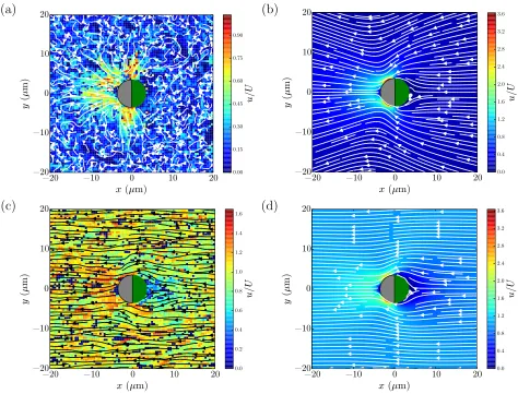
We show the experimentally measured flow fields in Figs. 1(c) and 1(d) (see [21] for zoom-out versions). It is apparent that the stuck particle [Fig. 1(c)] acts as a catalytic pump. Streamlines and velocity magnitudes indicate that the fluid is drawn in towards the equatorial region of the static Pt-PS particle and then pushed away from the Pt catalyst coated hemisphere. The pumping direction (away from Pt cap) is consistent with the direction of travel observed here, and reported previously [22]. In regions of low velocity, such as in the fluid surrounding the inactive side of the Pt-PS particle, Brownian translations of the tracer particles influence the streamlines producing stochastic detail,

−40 −20 0 20 40

−1

−0.5 0 0.5

x(µm)

ux ( x ) /U (a)

−40 −20 0 20 40

−2

−1.5

−1

−0.5 0 0.5

x(µm)

ux ( x ) /U (b)

−40 −20 0 20 40

−1

−0.5 0 0.5 1

y(µm)

uy ( y ) /U (c)

−40 −20 0 20 40

−1

−0.5 0 0.5

y(µm)

[image:3.612.72.299.331.385.2]

uy ( y ) /U (d)

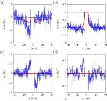
FIG. 2. Top: x-component of the velocity measured aty= 0 and as a function of the coordinatexfor the two situations where the swimmer is stuck (a) and freely moving (b). Bot-tom: y-component of the velocity measured atx= 0 and as a function of the coordinatey for the two situations where the swimmer is stuck (c) and freely moving (d). For all plots, the blue symbols and error bars are obtained experimentally after averaging the fields measured in a stripe of width 2µm aroundy= 0 (top) andx= 0 (bottom). The red line is a fit of the experimental data using the expressions of the velocity given in the Supplemental Information [21], withK =v0/U

as a free parameter. The expansions in Legendre polynomials are truncated at orderN= 25. The values of the fit param-eters are respectivelyK= 6.21 (a), 14.28 (b), 16.18 (c) and 8.92 (d).

Comparison with the theoretical predictions finds a good qualitative agreement between the structures of the flow field around the swimmer. In order to check quantitative agreement, and to observe more thoroughly the decay of the flow field far away from the surface of the colloid, we study different projections of the velocity field, namelyux as a function ofxaroundy= 0 anduy

as a function of y around x = 0 for the two situations (Fig. 2). To improve the statistics of the measurements, we average the velocity fields over stripes of width 2µm around y = 0 and x= 0. These results are fitted with the components of the flow fields computed analytically with K = v0/U [Eq. (2)] as a free parameter. All resulting fits yieldKvalues of order 10, as expected.

Discussion.— The very good quantitative agreement between the components of the velocity measured ana-lytically and experimentally shows that the simple shape of the slip velocity [Eq. (2) and Fig. 1(a)] correctly cap-tures the decay of the velocity field from the surface all the way to regions far from the Pt-PS particle, which is strongly in favor of the mechanism proposed in [11, 15]. The flow fields around a stuck or a moving swimmer for other candidate slip velocity profiles do not show a simi-larly good agreement in comparison [21]. A slip velocity that is fore-aft symmetric with a peak at the equator and that vanishes at the poles, which corresponds to a source dipole, does not yield the right structure for the flow field (in particular because the projection ofualong

y vanishes at x=z = 0). A profile of slip velocity that would be uniform on the Pt hemisphere and zero on the PS hemisphere will yield velocity profiles that are closer to the ones observed experimentally (even though there is no underlying theoretical mechanism to support this profile). However, the scenario corresponding to the ex-istence of current loops near the Pt hemisphere [Eq. (2)] offers even better fits of the experimental data.

In the context of comparison with theoretical veloc-ity profiles, experimental difficulties in determining fluid velocity in close proximity to the Pt-PS particle are rel-evant. In particular, the body of the Pt-PS colloid ham-pers tracking of the tracer colloids. For example some tracers pass below the equator of the Pt-PS particle and become obscured. This limits the number of tracer par-ticle trajectories that can be used to determine fluid ve-locity vectors in the very near field region. It should also be noted that in making a direct comparison with

the theoretical hydrodynamic predictions, we are neglect-ing any phoretic movement of the tracer particles due to the chemical gradients produced by the catalytically ac-tive particle. Additionally, determining the flow field us-ing tracer particles necessitated observation of the Pt-PS particle close to a 2D substrate. While the Pt-PS particle can move freely in 3D in bulk solution, the additional de-grees of rotational freedom, change in height relative to the microscope objective, and background tracer fluores-cence hamper 3D bulk solution flow field measurements. For these reasons, the fitting parameter K has a scat-ter around a number of order 10, which agrees with the expected order of magnitude.

Our observations are consistent with a velocity pro-file that behaves as a pusher in the far-field limit [21], which which can be a starting point for a description of the hydrodynamic interactions between many such self-phoretic active colloids [23–26]. However, our experi-ments have provided a more complete picture with re-gards to the near-field properties of the hydrodynamic interactions than a simplistic squirmer of pusher type, which can be used to build a more faithful representation of the hydrodynamic interactions. Therefore, our results will pave the way for a more comprehensive description of the self-organization of such active colloids through hydrodynamic and phoretic interactions [27, 28].

In conclusion, we have examined the hydrodynamic flow fields around a self-propelled Pt-PS catalytic active colloid and found flow fields that are strongly asymmetric across the surface of the particle, with larger magnitude on the Pt-coated hemisphere. The experimental mea-surements show good agreement with the explicit solu-tion of the Stokes equasolu-tion with a simple slip velocity as a boundary condition, which is consistent with the conjec-tured current loops. Our results can be used to construct a comprehensive theoretical description of a suspension of such active colloids.

ACKNOWLEDGMENTS

Both AIC and SJE thank the EPSRC for support-ing this work via the Career Acceleration Fellowship (EP/J002402/1) granted to SJE. PI and RG would like to thank the hospitality of the Max-Planck-Institute for the Physics of Complex Systems, where a part of this work was performed. We acknowledge support from the COST Action MP1305 Flowing Matter.

[1] F. Wong, K. K. Dey, and A. Sen, Ann. Rev. Mater. Res. 46, 407 (2016).

[2] C. Bechinger, R. Di Leonardo, H. L¨owen, C. Reichhardt, G. Volpe, and G. Volpe, Rev. Mod. Phys. 88, 045006 (2016).

[3] P. Illien, R. Golestanian, and A. Sen, Chem. Soc. Rev. 46, 5508 (2017).

[4] B. V. Derjaguin, G. P. Sidorenkov, E. A. Zubashchenkov, and E. V. Kiseleva, Kolloidn. Zh.9, 335 (1947). [5] N. O. Young, J. S. Goldstein, and M. J. Block, Journal

of Fluid Mechanics pp. 350–356 (1959).

[6] J. Anderson, Annual Review of Fluid Mechanics21, 61 (1989).

Rev. Lett. 94, 220801 (2005).

[8] R. Golestanian, T. B. Liverpool, and A. Ajdari, New Journal of Physics9, 126 (2007).

[9] W. F. Paxton, K. C. Kistler, C. C. Olmeda, A. Sen, S. K. St. Angelo, Y. Cao, T. E. Mallouk, P. E. Lammert, and V. H. Crespi, Journal of the American Chemical Society 126, 13424 (2004).

[10] J. R. Howse, R. A. L. Jones, A. J. Ryan, T. Gough, R. Vafabakhsh, and R. Golestanian, Phys. Rev. Lett.99, 048102 (2007).

[11] S. Ebbens, D. A. Gregory, G. Dunderdale, J. R. Howse, Y. Ibrahim, T. B. Liverpool, and R. Golestanian, Euro-phys. Lett.106, 58003 (2014).

[12] A. Brown and W. Poon, Soft matter10, 4016 (2014). [13] A. T. Brown, W. C. K. Poon, C. Holm, and J. D. Graaf,

Soft Matter13, 1200 (2017).

[14] Y. Ibrahim, R. Golestanian, and T. B. Liverpool, J. Fluid Mech.828, 318 (2017).

[15] S. Das, A. Garg, A. I. Campbell, J. Howse, A. Sen, D. Velegol, R. Golestanian, and S. J. Ebbens, Nat. Com-mun.6, 8999 (2015).

[16] K. Drescher, R. E. Goldstein, N. Michel, M. Polin, and

I. Tuval, Phys. Rev. Lett.105, 168101 (2010).

[17] A. I. Campbell and S. J. Ebbens, Langmuir 29, 14066 (2013).

[18] J. C. Crocker and D. G. Grier, Journal of Colloid and Interface Science179, 298 (1996).

[19] M. J. Lighthill, Commun. Pur. Appl. Math. 109, 109 (1952).

[20] J. R. Blake, J. Fluid Mech.46, 199 (1971). [21] See Supplemental Material for more details.

[22] S. J. Ebbens and J. R. Howse, Langmuir 27, 12293 (2011).

[23] F. J¨ulicher and J. Prost, The European Physical Journal E29, 27 (2009).

[24] Tu, Mei Hsien, PhD thesis, University of Sheffield (2013). [25] M. Yang and M. Ripoll, Soft Matter10, 6208 (2014). [26] P. Kreissl, C. Holm, and J. D. Graaf, J. Chem. Phys.

144, 204902 (2016).

[27] A. Z¨ottl and H. Stark, J. Phys. Condens. Matter 28, 253001 (2016).

Experimental Observation of Flow Fields Around Active Janus Spheres

Supplemental Material

Andrew I. Campbell,1 _{Stephen J. Ebbens,}1 _{Pierre Illien}2,3,4 _{and Ramin Golestanian}2

1_{Department of Chemical and Biological Engineering, University of Sheffield}

Mappin Street, Sheffield S1 3JD, UK

2_{Rudolf Peierls Centre for Theoretical Physics, University of Oxford, Oxford OX1 3NP, UK} 3_{Max Planck Institute for the Physics of Complex Systems, Nothnitzer Str. 8, 01187 Dresden, Germany}

4_{ESPCI Paris, UMR Gulliver, 10 Rue Vauquelin, 75005 Paris, France}

I. SOLUTION OF THE STOKES PROBLEM

A. Stuck swimmer

The total flow field around a stuck Janus swimmer reads

u=uph+umono, (S1)

where

• uph_{is the phoretic contribution (whether electrophoretic or diffusiophoretic),}

• umono_{is the contribution from the force monopole that maintains the colloid steady in the laboratory reference} of frame.

uph is the solution of the Stokes problem [Eq. (1) from the main text] with the boundary condition

uph_{θ |}r=a=

∞

X

n=1

BnVn(cosθ), (S2)

where

Vn(cosθ) =

2

n(n+ 1)sinθ P 0

n(cosθ). (S3)

The contribution from the force monopolef =−feˆ(f >0) is

umono =1

2

f

6πηacos(θ)

_a

r

3

−3a

r

ˆ

er+

1 4

f

6πηasin(θ)

_a

r

3

+ 3a

r

ˆ

eθ, (S4)

or, in dyadic notations,

umono=1

2 f 6πηa _a r 3

−3a

r

eˆ·r

r r r + 1 4 f 6πηa _a r 3

+ 3a

r

eˆ·r

r r r −eˆ

. (S5)

Using the known expression ofuph _{[19, 20], the total flow field then writes}

u=₋1

3

a3

r3B1eˆ+B1

a3

r3 ˆ

e_·r

r r r + ∞ X n=2

_an+2

rn+2 −

an rn

(Be

n+Bnd)Pn

_eˆ ·r r _r r + ∞ X n=2 n 2

an+2

rn+2 −

n

2 −1

an

rn

BnWn

_ˆ

e_·r

r

ˆ

e_·r

r r r −eˆ

(S6) +1 2 f 6πηa _a r 3

−3a

r

eˆ·r

r r r+ 1 4 f 6πηa _a r 3

+ 3a

r

eˆ·r

r r r −eˆ

, (S7)

with

Wn(cosθ)≡

Vn(cosθ)

sinθ =

2

n(n+ 1)P 0

(a)

−20

−10

0

10

20

x

(

µ

m)

−20

−10

0

10

20

y

(

µ

m)

0.00 0.15 0.30 0.45 0.60 0.75 0.90 u/U

(b)

−20

−10

0

10

20

x

(

µ

m)

−20

−10

0

10

20

y

(

µ

m)

0.0 0.4 0.8 1.2 1.6 2.0 2.4 2.8 3.2 3.6 u/U

(c)

−20

−10

0

10

20

x

(

µ

m)

−20

−10

0

10

20

y

(

µ

m)

0.0 0.2 0.4 0.6 0.8 1.0 1.2 1.4 1.6 u/U

(d)

−20

−10

0

10

20

[image:7.612.70.544.49.410.2]

x

(

µ

m)

−20

−10

0

10

20

y

(

µ

m)

0.0 0.4 0.8 1.2 1.6 2.0 2.4 2.8 3.2 3.6 u/U

FIG. S1. Zoomed-out version of Fig. 1. (a)-(d) Streamlines around the Janus particles obtained experimentally (left) and analytically (right), in the two situations where the particle is stuck (top) and freely moving (bottom). The background colors represent the magnitude of the velocityu=|u|rescaled by the swimming velocity of the Janus particle when it is freely moving.

The flow field at the surface of the colloid is

u_|r=aerˆ =−

f

6πηaeˆ+

2 3B1eˆ+

X

n≥2

BnVn(cosθ)ˆeθ. (S9)

Imposingf such that the swimmer does not move, we findf = 4πηaB1, and

u= 1

2B1

−a_r

ˆ

e+eˆ·r

r r r

+a

r

3

3eˆ·r

r r r −r

+ ∞ X n=2

an+2

rn+2 −

an rn

BnPn

_eˆ ·r r _r r + ∞ X n=2 _n 2

an+2

rn+2 −

n

2 −1

an

rn

BnWn

_eˆ

·r r

ˆ

e_·r

r r r −eˆ

(S10)

B. Moving swimmer: velocity field in the co-moving frame

Ignoring the contribution toucoming from the force monopole and solving the Stokes problem with the boundary condition

lim

−40 −20 0 20 40 −1

−0.5 0 0.5

x(µm)

ux

(

x

)

/U

(a)

−40 −20 0 20 40 −2

−1.5 −1 −0.5 0 0.5

x(µm)

ux

(

x

)

/U

(b)

−40 −20 0 20 40 −1

−0.5 0 0.5 1

y(µm)

uy

(

y

)

/U

(c)

−40 −20 0 20 40 −1

−0.5 0 0.5

y(µm)

uy

(

y

)

/U

[image:8.612.132.486.51.385.2]

(d)

FIG. S2. Top: x-component of the velocity measured aty = 0 and as a function of the coordinatexfor the two situations where the swimmer is stuck (a) and freely moving (b). Bottom: y-component of the velocity measured at x = 0 and as a function of the coordinateyfor the two situations where the swimmer is stuck (c) and freely moving (d). The red line is a fit of the experimental data using constant slip velocity over the Pt hemisphere [Eq. (S13)].

whereU = 2

3B1 is the swimming velocity of the colloid, we find

u=−2₃B1eˆ−

1 3

a3

r3B1eˆ+B1

a3

r3 ˆ

e_·r

r r r +

∞

X

n=2

an+2

rn+2 −

an rn

BnPn

_eˆ

·r r

_r

r

+ ∞

X

n=2

_n

2

an+2

rn+2 −

n

2 −1

an

rn

BnWn

_eˆ

·r r

ˆ

e_·r

r r r −eˆ

, (S12)

II. ADDITIONAL FIGURES

A. Enlarged view of the streamlines around the Janus particles

−40 −20 0 20 40 −1

−0.5 0 0.5

x(µm)

ux

(

x

)

/U

(a)

−40 −20 0 20 40 −2.5

−2 −1.5 −1 −0.5 0 0.5

x(µm)

ux

(

x

)

/U

(b)

−40 −20 0 20 40 −1

−0.5 0 0.5 1

y(µm)

uy

(

y

)

/U

(c)

−40 −20 0 20 40 −1

−0.5 0 0.5

y(µm)

uy

(

y

)

/U

[image:9.612.132.486.51.384.2]

(d)

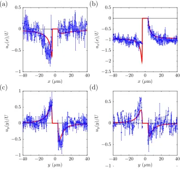
FIG. S3. Top: x-component of the velocity measured aty = 0 and as a function of the coordinatexfor the two situations where the swimmer is stuck (a) and freely moving (b). Bottom: y-component of the velocity measured at x = 0 and as a function of the coordinateyfor the two situations where the swimmer is stuck (c) and freely moving (d). The red line is a fit of the experimental data using constant slip velocity over the Pt hemisphere [Eq. (S14)].

B. Flow fields generated by alternative simple slip velocity profiles

1. Slip velocity with a dipolar symmetry

The flow field generated by the nonzero slip velocity at the surface of the colloid can again be calculated Eqs. (S10) and (S12), but with another expression for the slip velocity at the surface of the colloid [see Eq. (2) in the main text]. We first consider a slip velocity with a dipolar symmetry, that is peaked at the equator of the particle and vanishes at its poles:

uph_|r=a =v0sinθeθˆ (S13)

The velocity profiles ux(x, y = 0, z = 0) and uy(x= 0, y, z = 0) can be calculated and fitted to the experimental

measurements usingv0 as a fit parameter (Fig. S2). The results are commented in the main text.

2. Constant slip velocity over the Pt hemisphere

We then consider a slip velocity that is constant over the Pt hemisphere:

uph_|r=a=

(

v0eˆθ forπ/2< θ < π,

Although this is not an existing prediction for the system of Pt-PS colloid, we believe its comparison with the model that is based on current loops will be helpful. The velocity profiles ux(x, y= 0, z = 0) anduy(x= 0, y, z = 0) can

be calculated and fitted to the experimental measurements using v0 as a fit parameter (Fig. S3). The results are commented in the main text.

III. RELATIONSHIP WITH THE SQUIRMER MODEL CLASSIFICATION

Using Eq. (2) in the main text and the expansion given in Eq. (S2), we can calculate the first two moments of the slip velocity as

B1=

1 4 −

3π

64

v0, (S15)

B2=

1 2 −

15π

16

v0, (S16)

which yield a ratio of

β = B2 |B1| ' −

2.3, (S17)