Jochen Hinkel1,2 , John A. Church3 , Jonathan M. Gregory4,5 , Erwin Lambert6 , Gonéri Le Cozannet7 , Jason Lowe5,8 , Kathleen L. McInnes9 , Robert J. Nicholls10 , Thomas D. van der Pol1 , and Roderik van de Wal6,11
1Global Climate Forum (GCF), Berlin, Germany,2Division of Resource Economics, Albrecht Daniel Thaer‐Institute and Berlin Workshop in Institutional Analysis of Social‐Ecological Systems (WINS), Humboldt‐University, Berlin, Germany, 3Climate Change Research Centre, University of New South Wales, Sydney, Australia,4NCAS, University of Reading, Reading, UK,5Met Office Hadley Centre, Exeter, UK,6Institute for Marine and Atmospheric Research Utrecht, Utrecht University, Utrecht, The Netherlands,7BRGM, French Geological Survey, Orléans, France,8Priestley International Centre for Climate, University of Leeds, Leeds, UK,9CSIRO Oceans and Atmosphere, Aspendale, Australia,10School of Engineering, University of Southampton, Southampton, UK,11Geosciences, Physical Geography, Utrecht University, Utrecht, Netherlands
Abstract
Despite widespread efforts to implement climate services, there is almost no literature that systematically analyzes users' needs. This paper addresses this gap by applying a decision analysis perspective to identify what kind of mean sea level rise (SLR) information is needed for local coastal adaptation decisions. Wefirst characterize these decisions, then identify suitable decision analysis approaches and the sea level information required, andfinally discuss if and how these information needs can be met given the state of the art of sea level science. Wefind that four types of information are needed: (i) probabilistic predictions for short‐term decisions when users are uncertainty tolerant; (ii) high‐end and low‐end SLR scenarios chosen for different levels of uncertainty tolerance; (iii) upper bounds of SLR for users with a low uncertainty tolerance; and (iv) learning scenarios derived from estimating what knowledge will plausibly emerge about SLR over time. Probabilistic predictions can only be attained for the near term (i.e., 2030–2050) before SLR significantly diverges between low and high emission scenarios, for locations for which modes of climate variability are well understood and the vertical land movement contribution to local sea levels is small. Meaningful SLR upper bounds cannot be defined unambiguously from a physical perspective. Low‐to high‐end scenarios for different levels of uncertainty tolerance and learning scenarios can be produced, but this involves both expert and user judgments. The decision analysis procedure elaborated here can be applied to other types of climate information that are required for mitigation and adaptation purposes.Plain Language Summary
Information on future sea‐level rise (SLR) is needed for diverse coastal adaptation decisions such as deciding on how much sand to apply for counteracting beach erosion, designing the height and strength of coastal protection infrastructure, and planing future developments in the coastal zone. Different kinds of decisions thereby require different kinds of SLR information and not all kinds of information required can be delivered by the state‐of‐the‐art of sea‐level rise science. This paper addresses this problem from the points of view of both decision science and sea‐level rise science. Wefind that three kinds of SLR information can be produced to inform coastal decision making. First, probabilistic predictions of mean SLR can be produced for short term decisions (i.e., 2030‐2050) and some locations. Second, high‐end sea‐level rise scenarios chosen for different levels of uncertainty tolerance of decision makers can be developed by SLR experts assigning confidence levels to available SLR studies. Third, learning scenarios estimating what will be known about SLR at given points in the future can further improve decision making. The procedure elaborated in this paper can be applied to other types of climate information such as temperature or precipitation.1. Introduction
The core aspiration of developing climate services is meeting user needs for climate information. For sea level rise (SLR), such efforts have a long history dating back to the 1980s, with the U.S. Environmental
©2019. The Authors.
This is an open access article under the terms of the Creative Commons Attribution‐NonCommercial‐NoDerivs License, which permits use and distri-bution in any medium, provided the original work is properly cited, the use is non‐commercial and no modifica-tions or adaptamodifica-tions are made.
Key Points:
• Different kinds of contexts require different kinds of sea level rise information to support coastal adaptation decision making • Uncertainty intolerant users require
high‐end and low‐end sea level rise scenarios produced for different levels of uncertainty intolerance • Long‐term decisions can be
improved through learning scenarios estimating what will be learned about sea level rise in the future
Supporting Information:
•Supporting Information S1
Correspondence to:
J. Hinkel,
Citation:
Hinkel, J., Church, J. A., Gregory, J. M., Lambert, E., Le Cozannet, G., Lowe, J., et al. (2019). Meeting user needs for sea level rise information: A decision analysis perspective.Earth's Future,7, 320–337. https://doi.org/10.1029/ 2018EF001071
Received 15 OCT 2018 Accepted 26 FEB 2019
Protection Agency guidance by Hoffman et al. (1983) and the U.S. National Academy of Science guidance on “Responding to Sea‐level rise”(NRC, 1987) published 7 and 3 years before thefirst Intergovernmental Panel on Climate Change (IPCC) report (Houghton et al., 1990), respectively. In recent years, the provision of SLR information for coastal adaptation has grown considerably, with prominent efforts including the Dutch Delta Commission (Katsman et al., 2011), SLR scenarios for Australia (McInnes et al., 2015), the U.K. SLR scenarios (Lowe et al., 2009), and the United States Army Corps of Engineers guidance (USACE, 2011). Across those efforts, it is generally recognized that providing useful SLR information requires codevelop-ment between researchers and users (Le Cozannet, Nicholls, et al., 2017; Oppenheimer & Alley, 2016).
Despite these efforts, there has been little empirical and systematic exploration of what kind of SLR information users need. Many studies in the academic literature claim that they are motivated by addressing adaptation user needs, without providing any empirical evidence of these needs (e.g., Grinsted et al., 2015; Jevrejeva et al., 2016; Kopp et al., 2014; Le Bars et al., 2017). Empirical investigations of user needs, either by analyzing the kind of SLR information users employ (Le Cozannet, Manceau, & Rohmer, 2017; Le Cozannet, Nicholls, et al., 2017) or asking users what kind of information they would employ (Tribbia & Moser, 2008), are relatively scarce. More such efforts are needed to broaden the empirical understanding of user needs.
Asking users is, however, not the only strategy for systematically identifying SLR information needs, and this may even lead to the production of misleading SLR information, due to well‐documented deficits in individual and social choice. On an individual level this includes, for example, systematic cognitive biases that may prevent users from asking for the right piece of SLR information (Tversky & Kahneman, 1974). On a social level this includes opportunistic behavior of self‐interested individuals or lobby groups shaping political processes and thus limiting the ability to act in the social interest (Levine & Forrence, 1990). For example, the use of certain emission or SLR scenarios may be prescribed by regulation.
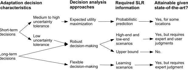
This paper follows a complementary strategy for systematically identifying SLR information needs by taking users' decisions rather than users'final information needs as entry points and applying decision analysis (DA) thinking. This strategy is meaningful, because different decisions require different DA methods, which in turn require different kinds of information (Kleindorfer et al., 1993). Here we follow this procedure (Figure 1) byfirst characterizing coastal adaptation decisions (section 3), then discussing available DA methods and SLR information appropriate for these (section 4), andfinally discussing how these informa-tion needs can be met given the state of the art in sea level science (secinforma-tion 5) Figure 2. To handle the con-tested terminology used within and across the differentfields of scholarship involved in this procedure, we define relevant terms of DA and uncertainty characterization upfront (section 2).
Note that a DA perspective as elaborated here focuses on the analytical aspects of SLR information and decision making. Beyond this there are other aspects that need to be considered, such as risk communica-tion and stakeholder engagement processes. While these aspects fall beyond the scope of this paper, the DA perspective offers a framework that can be used within stakeholder processes to address some of the short-comings of decision making pointed out above. While we address information needs for coastal adaptation, the general approach taken in this paper is applicable to other areas of climate change adaptation and mitigation.
2. Terminology
2.1. Decision Analysis
2.2. Uncertainty Characterization
Dealing with uncertainty is a key to DA, and different ways of characterizing uncertainty are used for repre-senting future SLR and analyzing decisions. As the terminology in the literature is ambiguous, we define the key terms used in this paper.
On a basic level, uncertainty may be characterized in terms of what is possible. Uncertainty, in a real num-ber, for example, may be bounded iflower boundsandupper boundscan be given, whereas any number higher (lower) than what is possible is called an upper (lower) bound. If all possibilities are known, uncer-tainty can be represented as anuncertainty interval[a,b] with agreatest lower bound aand aleast upper bound b, giving the lowest and highest possible SLR at a given points in time, respectively. When the full range of uncertainty cannot be specified, as is generally the case for variables associated to human develop-ment, uncertainty may be represented byscenarios, which are sets of plausible examples of how the future may unfold (Kahn & Wiener, 1967).
Uncertainty may also be characterized in terms of what is probable by providing a single probability density function over the uncertainty interval. Here this is calledprobabilistic prediction. Note that the atmospheric and ocean weather and climate community defines probabilistic prediction in a more narrow sense as“the result of an attempt to produce (starting from a particular state of the climate system) an estimate of the actual evolution of the climate in the future, for example, at seasonal, inter‐annual, or decadal time scales.” (IPCC, 2013) In our paper, we use probabilistic prediction in the wider sense as used in decision sciences, independent from the method applied to produce a prediction (e.g., independent from whether simulations start from an observed state of the climate system or not; van der Pol & Hinkel, 2019).
In the domain of climate change and SLR, uncertainty is often represented in the form ofprobabilistic scenarios, which are probability distributions over possible values of climate variables (e.g., sea level) at given points in time conditional on an emission, concentration, or radiative forcing scenario (IPCC, 2013). The dashed probability distributions in Figure 2 provide an illustration of probabilistic scenarios. Generally, the probability distributions are given pointwise. Jackson and Jevrejeva (2016), for example, provide future SLR for each Representative Concentration Pathway (RCP) through 6 points of the distribution (i.e., the 5th, 17th, 50th, 83rd, 95th, and 99th percentiles).
A further distinction important for this paper is the one betweenshallow
anddeepuncertainty. The former is the situation in which a single unam-biguous probability distribution can be attached to states of the world (here local mean SLR), and the latter the situation in which this is not possible, because parties cannot agree on an unambiguous method for deriving probabilities, or their subjective probability judgments differ (Kwakkel et al., 2010; Lempert & Schlesinger, 2001; Weaver et al., 2013).
[image:3.612.220.529.91.206.2]Specifically for SLR, high‐end scenarios (and, more rarely, low‐end scenarios) are used to represent possible high‐end (low‐end) SLR (Katsman et al., 2011; Lowe et al., 2009). What high end or low end means cannot be defined formally based on possibilities or probabilities. These
Figure 1.Applicable decision analysis approaches and corresponding sea level information requirements, depending on the decision horizon of coastal adaptation decisions and the uncertainty tolerance of users.
[image:3.612.41.285.576.714.2]notions have been put forward precisely because both possibilities and probabilities are difficult to establish for the case of SLR as discussed in section 4.
Finally, in some DA,learning scenarioscan be used, which are sets of scenarios estimating SLR information plausibly available at a given point in time in the future (e.g., in 2050) about SLR beyond that point of time (i.e., beyond 2050). Figure 3 provides a conceptual example of such learn-ing scenarios, which consider different uncertainty ranges for the sea level projections that will be available in the future.
3. Coastal Adaptation Decisions
Here we define coastal adaptation to include both adaptation to current and to future mean and extreme sea level events such as storm tides. We combine these two aspects, because in practice there are hardly any “pure” coastal adaptation decisions addressing SLR only. Many coasts are already risky places today threatened by extreme sea levels that result from combinations of storm surges, tides, waves, and river discharge and seasonal to interannual variability (Wong et al., 2014).
Coastal decisions differ in many aspects, two of which are specifically relevant for choosing appropriate DA frameworks and providing SLR information. Thefirst aspect is the decision horizon, which refers to the planning times, response times, and lifetimes of all alternatives considered in a decision. Some coastal deci-sions are short term, defined here as decision horizon below 30 years. This includes, for example, shore and beach nourishment, which counteract coastal erosion orflooding through artificially replacing eroded sand and other materials. Nourishment decisions could be annual decisions but are usually repeated activities within projects that may have lifetimes of a decade or two (Stive et al., 2013).
Longer‐term decisions, defined here as those with decision horizon longer than 30 years, includeflood pro-tection and other infrastructure and spatial planning decisions. Coastal propro-tection infrastructure such as dikes, seawalls, and breakwaters usually involve decision horizons of 30 to 100 years and more (Burcharth et al., 2014). Major protection infrastructure such as storm surge barriers generally takes decades to plan and implement and hence may be built for even longer lifetimes (Gilbert & Horner, 1986). Decision horizons of over 100 years are associated with some critical infrastructure with long lifetimes, most espe-cially nuclear power plants (Wilby et al., 2011). Similarly, land use planning, coastal risk zoning, and coastal realignment decisions (Hino et al., 2017) may have effects that last several decades extending to over a century.
The second aspect specifically relevant for choosing appropriate DA frameworks and SLR information is uncertainty tolerance, which refers to the level of uncertainty a user is willing to accept (Kunreuther et al., 2013). The lower the uncertainty tolerance, the more the user will do to avoid being exposed to uncer-tainty, and this needs to be considered when analyzing decisions. People are generally more uncertainty tol-erant if the value at risk is relatively low. Conversely, people living in coastal areas with high densities of populations and assets generally have a low uncertainty tolerance and prefer to protect these areas against unlikely but possible extreme SLR (Hinkel et al., 2015; Lowe et al., 2009). Uncertainty tolerance is at its lowest when it comes to critical infrastructure with long lifetimes, such as nuclear power plants (Wilby et al., 2011).
[image:4.612.41.286.90.221.2]Uncertainty tolerance and perception vary both within and across societies. For example, coastal risk per-ception can vary with gender, environmental attitudes, and political orientation (Carlton & Jacobson, 2013). Coastal uncertainty tolerance generally decreases with economic development (Hinkel et al., 2014) and increases after a coastal disaster has been experienced (Cassar et al., 2017). On a social level, different levels of uncertainty tolerance are revealed across countries through different coastal protection standards and degrees to which this is formalized into law (Van der Most & Schasfoort, 2014). Coastal protection stan-dards differ significantly across global coastal megacities even under similar exposure and wealth (Hallegatte et al., 2013).
4. DA Approaches and Corresponding Information Needs
This section briefly presents widely used DA approaches and maps these to the kinds of coastal decisions identified above (Figure 1). We distinguish between three general classes of DA methods. Practical cases may have elements of all three classes rather than focusing on just one. For each class we consider what SLR information would be required, and in the section 4 we consider if SLR science can provide this information.
4.1. Expected Utility Maximization Versus Robust Decision Making
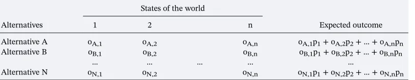
A major criterion for the applicability of DA approaches is whether one is confronted with a situation of shallow or deep uncertainty (see definitions in section 2.2). In situations of shallow uncertainty, approaches thatmaximize expected utility(also called risk‐based approaches) are suitable. The objective of these methods is to identify the adaptation alternative that has the best expected outcome, which is the probability‐ weighted sum of all outcomes of an alternative in all states of the world (Briggs, 2017; Simpson et al., 2016). The expected outcome measure thus attained for each deep alternative can be used for ranking alter-natives across scenarios and choosing the best one (Table 1). A prominent example of this approach is a cost‐ benefit analysis (CBA) under probabilistic uncertainty (Graham, 1981), which maximizes expected NPV (the discounted stream of net benefits). The information required for applying this approach in the context of SLR is an unambiguousprobabilistic predictionof future sea levels (section 2.2).
In situations of deep uncertainty, expected outcomes cannot be computed, and alternatives cannot be ranked across states of the world. Alternative approaches calledrobust decision making (RDM) can be applied and have been promoted specifically for climate change related decisions due to the deep uncertainty in emission, mitigation, and socioeconomic scenarios (Heal & Millner, 2014; Lempert & Schlesinger, 2001). The objective of RDM is to identify alternatives that perform reasonably well, that is, arerobust, under a wide range of future states of the world. This includes so‐called exploratory modeling methods that rely on simu-lation models to create large ensemble of plausible future scenarios for each alternative and then use search and visualization techniques to extract robust alternatives (Lempert & Schlesinger, 2000). A range of attri-butes such as costs, benefits, regret, reversibility, and security margins may be considered to characterize alternatives and define robustness criteria (McPhail et al., 2018). Used in a wider sense, RDM also includes methods that follow similar ideas (Hall et al., 2012; Roach et al., 2016) such as robust optimization (Ben‐Tal et al., 2009), info gap theory (Ben‐Haim, 2006), and decision analyses employing robust decision criteria such as minimax and minimax regret (Niehans, 1948; Savage, 1951). The SLR information required for RDM approaches is high‐end SLR scenarios and, for some methods such as robust optimization and mini-max regret, also low‐end SLR scenarios. The more uncertainty intolerant users are the higher (lower) and, more unlikely, the high‐end (low‐end) scenario should be. If users are very uncertainty intolerant, the best piece of information for RDM would be an upper bound for SLR (Hinkel et al., 2015).
[image:5.612.176.582.115.194.2]A second criterion for choosing between expected utility approaches and RDM approaches is uncertainty tolerance. When stakeholders have a low uncertainty tolerance, expected utility approaches are generally less suitable, because the goal of uncertainty intolerant decision makers may be to avoid major damages under worst case or a wide range of circumstances. An adaptation strategy developed based on the
Table 1
Illustration of a Decision Problem Under Uncertainty
Alternatives
States of the world
Expected outcome
1 2 n
Alternative A oA,1 oA,2 oA,n oA,1p1+ oA,2p2+…+ oA,npn Alternative B oB,1 oB,2 oB,n oB,1p1+ oB,2p2+…+ oB,npn
… … … … …
Alternative N oN,1 oN,2 oN,n oN,1p1+ oN,2p2+…+ oN,npn
maximization of expect utility may not fullfil such goals, because high‐end damages occurring can exceed expected damages by orders of magnitude. For example, a CBA mayfind that a dike that protects against the 1,000‐yearflood has the highest expected net benefits, but the damages of a 10,000‐yearflood may still be unacceptable to society. To some extent, uncertainty intolerance can be considered in expected utility methods through a risk premium, sensitivity analysis, and so forth (e.g., Pratt, 1964; Tversky & Kahneman, 1992), but if uncertainty tolerance is low, RDM methods may be a better choice.
Inflood risk management practice, scenario‐based CBA is often used, which is an approach that sits between expected utility maximization and RDM (HMT, 2007; Romijn & Renes, 2013). Here expected aggregated utility (as NPV) is computed but only within each scenario and not across scenarios. Hence, this approach cannot uniquely rank alternatives to identify the one with the highest expected utility across states of the world. However, the results of this approach (i.e., one NPV for each combination of alternatives and scenar-ios) can inform decision makers in their choice and/or can be used as attributes in RDM approaches.
4.2. Flexible Decision Making
Both optimal and RDM methods can be combined withflexible decision‐making approaches that are applic-able if there is the opportunity of learning more about sea levels within the time horizon of the coastal adap-tation decision. Given the large uncertainties in future sea levels and the long decision horizons involved in many coastal adaptation decisions, a meaningful strategy is to break decisions down into stages and favor
flexible alternatives over nonflexible ones, in order to delay decisions where possible until more is known about SLR (Hallegatte, 2009). For example, aflexible protection approach would be to build small dikes on foundations designed for higher dikes, wait to see how SLR unfolds, and if necessary raise the dike further at a later stage. A prominent and lightweight method that addresses the objective offlexibility is adaptation pathway analysis (Haasnoot et al., 2011). The SLR information needed for this method is similar to one of RDM discussed above.
There is, however, another class of DA methods that goes further than adaptation pathways and brings along new requirements for SLR information. Adaptation pathway analysis cannot answer the question of how muchflexibility and what timing of adaptation is economically efficient or robust. Delaying decisions and opting forflexible alternatives generally introduces extra costs, because (a)flexible alternatives are often more expensive than their inflexible counterparts and (b) expectedflood damages increase if a decision is postponed. An important consideration therefore is to balance the cost of delaying decisions with the
bene-fits of deciding later when more information is available. This is precisely the decision problem that real‐ options analysis (Dixit & Pindyck, 1994) and decision‐tree analysis (Conrad, 1980) can address. The former is an extension of CBA with the arrival of new information and thus can only be applied when probabilistic predictions are available as discussed above.
The application of real‐options analysis and decision‐tree analysis to assess the trade‐off between adapting now or in the future requires what can be called second‐order sea level information or learning information, that is, scenarios of what kind of information we are likely to have in the future (e.g., in 30 years) about future SLR (i.e., beyond 30 years). See Figure 3 for an example.
5. Meeting the Identi
fi
ed Needs
This section explores, for each of the four SLR information requirements identified in the last section (Figure 1), to what extent these needs are or can be met given the state of the art of SLR science.
5.1. Probabilistic Sea‐Level Predictions
For scenario uncertainty, objective probabilities cannot be derived; otherwise, scenarios would not be used in thefirst place. Whether subjective probabilities can, or should, be attached to emission scenarios has been extensively debated in the climate change community. The main argument in favor of attaching subjective probabilities is that decision makers might misinterpret the absence of probabilities as the emission scenar-ios being equally likely (Schneider, 2001). Arguments against this include that the space of possible future emissions is insufficiently sampled by any number of scenarios and individuals are likely to significantly disagree on subjective probabilities of emission scenarios (Lempert & Schlesinger, 2001; Stirling, 2010). The latter arguments seem to have won the debate, at least only a few studies that have attached subjective probabilities to emission/mitigation scenarios exist in the climate impact literature. In the SLR rise‐related decision‐making literature, examples of assigning equal probabilities to climate scenarios (Michelle Woodward et al., 2014), non‐equal probabilities (Abadie, 2018), and multiple sets of subjective probabilities (Dawson et al., 2018) can be found.
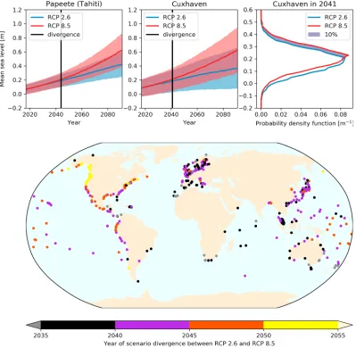
Without probabilities for emission scenarios, future sea levels can only be characterized as a single unambig-uous probability distribution if scenario uncertainty is small enough and can be ignored. Small enough in the context of expected utility approaches means that the results are insensitive to the choice of the scenario, because SLR projections do not significantly diverge between the lowest and highest emission/concentration scenarios. Until the middle of the century, differences between global mean SLR projections due to differ-ences in scenarios are generally small (Garner et al., 2018; Horton et al., 2018), but the point in time when scenarios diverge differs across locations and depends on the metric applied for detecting divergence. As an illustration, we take the Fifth Assessment Report (AR5) SLR projections (Church et al., 2013) together with interannual sea level variability from global tide gauge stations from Woodworth et al. (2016), to assess the year of scenario divergence, using a 10% threshold in the statistical distance between the distributions of RCP2.6 and RCP8.5 (Figure 4). We consider only the upper half of the distributions, as we are interested in an upward shift of the RCP8.5 distribution relative to the RCP2.6 distribution and not so much in changes in shape. See the supporting information for details on methods applied. The year of scenario divergence var-ies geographically, as this depends on regionally varying SLR projections and on the variability of all sea level components, which differ across regions (Le Cozannet et al., 2015; Little et al., 2015). For 8% of the stations, divergence occurs before 2035, and for 9% of the stations, this occurs after 2050. The year of divergence can vary over short distances, because the local mean sea level variability can vary dependent on the specific pla-cement of the tide gauges stations. Such local variation can be seen, for example, along the U.S. East Coast.
The threshold of 10% is arbitrary and must be chosen with respect to the uncertainty tolerance of the involved stakeholders and other aspects of the decision context. The more tolerant stakeholders are to uncer-tainty, the larger the differences between SLR from high‐end and low‐end emission scenarios that can be accepted. We have chosen 10% as afirst signal that the distributions can no longer be considered indistin-guishable, because expected utility approaches normally take into account the damages resulting from extreme sea levels and small variations in mean SLR may have a large effect on the expectedflood damages of extremes. To test the sensitivity of the year of divergence to the choice of threshold and the inclusion of extremes, results for threshold values of 10% and 33% are compared in the supporting information.
limited predictability of wind and atmospheric variability in these regions (Roberts et al., 2016). The initialization to observed states becomes important for decision making if this step significantly alters the expected utility computed from the sea level distribution, which is the case when the internal variability is high as compared to other components of sea level change. Similarly to the case of scenario uncertainty discussed above, the higher the uncertainty tolerance of the user, the higher differences can be tolerated. In any case, an ensemble of climate models not initialized to the observed state can still be used to make probabilistic predictions on longer time scales before scenarios diverge.
[image:8.612.176.575.90.480.2]Regarding the vertical land movement component of local sea level change, paleo‐records and geodetic mea-surements can provide useful information on long‐term gradual vertical land movement (e.g., Horton et al., 2018; Wöppelmann & Marcos, 2016). However, future vertical land movements are especially difficult to quantify and can hardly be included in a probabilistic framework when the two following types of processes are involved. In tectonic active areas, vertical ground motion during or after earthquakes can lead to abrupt large changes in sea levels that are difficult to predict (Ballu et al., 2011). Similarly, human‐induced land subsidence due to drainage and groundfluid or gas abstraction can lead to rates of local SLR of 10 or
more times higher than those of climate chance induced SLR, especially in delta regions (Syvitski et al., 2009). Future rates are, however, difficult to predict because these depend on human behavior with regard to the extent by which this will be managed (Kaneko & Toyota, 2011). Uncertainties in glacial‐isostatic adjustment have been represented through probabilities by considering the difference between two models as the standard deviation of a Gaussian distribution, but this cannot give a robust distribution (Jevrejeva et al., 2014). The contribution of glacial‐isostatic adjustment to local sea level change is, however, generally small as compared to the other components of local sea levels (except in high‐latitude regions).
In summary, the current state of the art allows the generation of unambiguous probabilistic predictions and hence the application of expected utility approaches only
1. for the near term (i.e., 2030–2050, depending on the location) before SLR significantly diverges between low and high‐end emission scenarios, and
2. for regions for which tectonic activity and human‐induced subsidence play a minor role in determining local sea levels. This excludes deltas (due to high human‐induced subsidence) and places located close to faults or volcanoes, especially near plate boundaries (e.g., Japan, Indonesia, or the Antilles archipelago). In all other cases, it would be better to apply RDM approaches together with high‐and low‐end scenarios, as discussed in section 5.3. Toward this end, high‐and low‐end sea level outcomes for the near term can be generated by combining information from observations and model simulations, including seasonal and decadal forecasts, as demonstrated for precipitation in the United Kingdom (Thompson et al., 2017) and SLR in Australia (McInnes et al., 2015).
5.2. Upper Bound of SLR
As concluded in section 3, the ideal piece of information for RDM under low levels of uncertainty tolerance would be an upper bound of SLR for given points of time. In the literature there have been attempts to produce“upper bounds”for 21st century SLR based on paleo‐records and kinematic constraints on ice sheet discharge. In this literature, the term upper bound is, however, generally not used in the strict mathematical sense as used in this paper, but rather in the loose sense of what we call here a high‐end SLR scenario (see section 2.2.). For example, Pfeffer et al. (2008) conclude that“increases (in sea level by 2100) in excess of 2 meters are physically untenable”based on kinematic constraints in ice sheet discharge. It is, however, diffi -cult to define the concept of a physical upper bound unambiguously in a SLR context. On the one hand, 2 m by 2100 is not physically tenable in the sense of being inconsistent with the understanding at that time of the possible processes. On the other hand, one can argue that SLR of more than 2 m by 2100 is physically tenable in the sense that it does not violate physical laws such as conservation of mass and energy. Physically impos-sible would be a rise of, say, 80 m by 2100 because there is not enough ice stored on land, but this number would be of no value for a coastal planner.
In summary, at present we can construct high‐end scenarios that are consistent with limitations imposed by present understanding, but we cannot provide a true upper bound. This is not to say that the work trying to define“upper bounds”based on paleo‐records and kinematic constraints on ice sheet discharge is not help-ful for decision making. On the contrary, such results can, together with results of modeling studies, contri-bute to the generation of high‐end scenarios for users with different levels of uncertainty tolerances as discussed in the next subsection. For example, the work of Pfeffer et al. (2008) and the work of Rohling et al. (2008), who estimate a maximum of 2.5 m of global mean SLR per century during the last interglacial period, have been applied to develop what is termed the H++ high‐end scenario range (Lowe et al., 2009; Nicholls et al., 2014; Ranger et al., 2013). But more care should be taken in the usage of the term upper bound.
5.3. High‐End and Low‐End SLR Scenarios for Different Levels of Uncertainty Tolerance
For less uncertainty‐tolerant users, the situation is more complex, because uncertainty‐intolerant decision making also requires taking account of SLR beyond the likely range, as well as lower confidence lines of evidence that have not been included in the generation of the IPCC projections (Hinkel et al., 2015).
In recognition of this need other studies have generated percentiles beyond thelikelyrange byfitting prob-ability distributions to available data from model ensembles including the 17th and 83rd percentiles provide by AR5 (e.g., Grinsted et al., 2015; J. Hunter, 2012; J. R. Hunter et al., 2013; Jevrejeva, Moore, et al., 2014; Kopp et al., 2014; Le Bars et al., 2017; Le Cozannet et al., 2015; Nauels et al., 2017). The caveat of this approach is that there is lower confidence in the understanding of the physical processes contributing to SLR percentiles outside of thelikelyrange as compared to those processes contributing to SLR within the likely range. In addition, there is no physical reasoning for why the distribution should continue to hold its shape in the tails. For these reasons, the authors of the AR5 have included only thelikelyrange into their SLR scenarios, although they did consider the potential for a larger Antarctic contribution (Church et al., 2013).
To go beyond the likely range, studies have also drawn upon additional but lower confidence lines of evidence on the contribution of the Antarctic ice, which is the component of SLR contributing most to the distribution's tail‐end uncertainty. On the one hand, this includes studies that have used structured expert elicitation (e.g., Bamber & Aspinall, 2013; De Vries & Van de Wal, 2015; Grinsted et al., 2015; Horton et al., 2014; Jackson & Jevrejeva, 2016; Jevrejeva, Grinsted, et al., 2014; Kopp et al., 2014; Le Bars et al., 2017). Structured expert elicitation has been applied successfully for characterizing risks such as earth-quakes, volcanos, and dam failures (Aspinall, 2010) It has, however, been argued that this method is less applicable in areas in which social behavior influences outcomes, because experts lack so‐called predictive capabilities in these areas (Morgan, 2014). This is precisely the case for climate change, as its magnitude depends on GHG emissions and hence the mitigation behavior of society. Furthermore, there has been effec-tively no previous learning experience with the rapid changes in mean sea levels expected.
On the other hand, this includes studies that have used results of the new ice sheet model of DeConto and Pollard (henceforth DP16) to estimate contribution of the Antarctic ice (DeConto & Pollard, 2016; Kopp et al., 2014; Le Bars et al., 2017; Nauels et al., 2017). The projections of DP16 for Antarctic ice sheet mass
Figure 5.The construction of low‐end and high‐end mean SLR scenarios for 2100 (relative to 1986–2005) applicable in robust decision making for users with different levels of uncertainty tolerance. The ranges are derived by combing low-est (i.e., RCP2.6) and highlow-est (i.e., RCP8.5) cumulative probability distributions of studies with the same confidence levels into p‐boxes (shaded areas). The left panel shows the construction of a p‐box combining Kopp et al. (2017) and Le Bars et al. (2017), both based on the DeConto and Pollard (2016) and hence considered to be very low confidence studies. The right‐hand panel adds to this very low confidence p‐box (green area), a low confidence p‐box based on Kopp et al. (2014) and Jackson and Jevrejeva (2016) (red area), and a medium confidence p‐box based on the likely ranges of
loss are much higher than those of other recent publications (Golledge et al., 2015; Levermann et al., 2014; Ritz et al., 2015), because their model produces widespread early surface melting of ice shelves, leading to hydrofracturing and complete collapse (as occurred for the Larsen B ice shelf in 2002), and subsequent marine ice cliff instability (MICI) in many places. While this is physically plausible, this chain of processes has so far not been observed, and the most recent publications (Edwards et al., 2019; Golledge et al., 2019)
find a much smaller Antarctic contributions by 2100 as well as that it is not essential that the ice cliff mechanism is required to simulate paleo sea level observations. For those regions where Antarctica is currently retreating (Thwaites glacier in particular), the general understanding is that it is not due to the above mentioned chain of processes but rather due to enhanced basal melting below the ice shelves (Joughin et al., 2014; Rignot et al., 2014). Also, the currently available projections of the tails of the PDF have tended to use one input for Antarctica rather than the full suite of available information.
In summary, a dilemma remains. While uncertainty intolerant decision making requires SLR information beyond thelikelyrange, efforts to go beyond this range have serious caveats and hence provide lower confi -dence information. As a result, different studies provide very different SLR estimates for the same percentiles (Figure 5), and this is likely to continue to be the case in the future.
One strategy to address this dilemma offered by decision sciences is not to combine results of different stu-dies, model runs, or expert opinions but rather to report disaggregated results and document the reasons why these differ (Morgan, 2014; Stirling, 2010). For example, in the case of DP16, it could be documented that their results depend on a single model of a chain of processes that is plausible but has so far limited observa-tional evidence. The very uncertainty intolerant user could then decide to consider these lower confidence estimates. The main caveat associated with this strategy is that it requires well‐informed users.
An alternative strategy put forward by decision sciences in situations in which probabilities are poorly defined is to combine model runs, sea level components, and studies using reasoning based on extraprobabil-istic theories such as possibility theory or imprecise probability theory instead of probability theory (Dubois, 2007; Le Cozannet, Manceau, & Rohmer, 2017). For example, the probabilistic ranges (e.g., thelikelyranges) and the probabilistic projections provided by studies could be combined into a single probability box (p‐box) that gives the smallest and largest probability distribution for all studies considered. See Figure 5a for an illustration of this and Garner et al. (2018) for p‐boxes combining distributions from semiempirical and prob-abilistic studies published since AR5.
Similarly, ensemble maxima of various sea level components could be summed up to produce a high‐end SLR scenario (Jevrejeva, Grinsted, et al., 2014). If the component maxima are possible, then the sum of these should also be possible, unless there is an anticorrelation among them. The same reasoning should also be applied to broaden the physical basis for producing high‐end SLR scenarios. Up to now, efforts such as the Coupled Model Intercomparison Project (Eyring et al., 2016) and Ice Sheet Model Intercomparison Project (Nowicki et al., 2016) have been established to provide information on the middle ranges or best estimates of distribution of climate variables. Alternative modeling experiments explicitly targeted at developing high‐end scenarios could be established, making worst‐case assumption for model parameters, initial condi-tions, and forcing. The main caveat of combining all expert opcondi-tions, model runs, and studies into a single p‐ box is that the resulting very wide uncertainty range is only useful for users with a low uncertainty tolerance.
The caveats of both of these strategies can be addressed, to the extent possible, by placing expert confidence judgments on different studies and only combining those studies that have the same confidence level (Figure 5). The confidence assigned to a study depends on lines of evidence informing a study and the extent to which they are consistent (Mastrandrea et al., 2011). We illustrate this by grouping a couple of recent studies into the following three confidence levels.
1. Medium confidence: First, we take the AR5 scenarios, which have not estimated probabilities beyond the likely range due to insufficient evidence available at the time of writing. We follow AR5 authors in assign-ing medium confidence to these.
confidence results, as discussed above. Note that the higher percentiles of Jackson and Jevrejeva lie above those of Kopp et al., because the former use the distributions of Bamber and Aspinall (2013) as is, while Kopp et al. (2014) scale the distributions to agree in their likely ranges with the AR5 ice sheet projections. Here we do not consider this difference as a necessary condition for opening up an additional group of studies.
3. Very low confidence: Third, we combine the probability distributions of studies based on DP16, notably Kopp et al. (2017) and Le Bars et al. (2017). We assign a very low confidence to these studies due to their results being conditional on a single and observationally poorly constrained line of evidence (i.e., a single ice sheet model), and the much lower projections from the most recent studies (Edwards et al., 2019; Golledge et al., 2019).
This categorization, together with the percentiles of the imprecise probability distributions thus attained for each category of confidence levels, can then be used for selecting low to high‐end SLR scenarios for RDM based on the uncertainty tolerances of users. The lower the uncertainty tolerance of a user is, the lower confidence level information should be taken into account (Figure 5).
Note that the categorization of studies into different groups of equal confidence is a dynamic and subjective task based on expert judgment. The categories applied, and the confidence judgments made, will vary in time as part of the progression in scientific understanding. This task cannot be avoided at this stage if SLR science shall be used to inform decisions, given the diversity of methodologies applied and ambiguity among the studies available. Furthermore, this task is already well established within assessments of scientific evi-dence such as the one of the IPCC. In addition, despite the subjectivity of this task, the scientific debate offers some clear‐cut criteria for classifying studies into different levels of confidence. At the time of writing of AR5, a main criterion was to distinguish studies based on process‐based models (judged to be of medium confi -dence) and those based on semiempirical models (judged to be of low confidence; Church et al., 2013). Post AR5, there have been several publications projecting the contribution of Antarctica through expert judgment and through the consideration of new processes such as MICI, which are the criteria applied here to constitute the confidence level categories.
Moreover, the procedure of categorizing studies and deriving low‐to high‐end scenarios for different levels of uncertainty tolerance needs to consider all relevant studies and methodologies for deriving sea level infor-mation, including those methods in which confidence is lower, such as semiempirical models, paleo‐records, and kinematic constraints on ice sheet discharge (Hinkel et al., 2015). One advantage of the proposed pro-cedure based on possibility reasoning is thereby that it can combine SLR information given in the form of probabilistic scenarios (i.e., the studies used in Figure 5) with nonprobabilistic information (e.g., the kine-matic constraints on ice sheet discharge by Pfeffer et al. as discussed above; Le Cozannet, Manceau, & Rohmer, 2017; Le Cozannet, Nicholls, et al., 2017).
Finally, a seeming caveat of this strategy based on possibilities is that probabilistic information is lost. From the adaptation perspective, however, the probabilities available through probabilistic scenarios have no direct meaning, because they are conditional on a given emission/mitigation scenario. For example, if one chooses the 95th percentile of SLR under RCP8.5, this does not mean that there is a 5% chance of SLR being higher than this. Under the assumption that RCP8.5 would be the highest possible GHG concentration scenario, the chance of exceeding the 95th percentile of RCP8.5 would be smaller than 5%. This assumption is, however, not evident. For example, it has been argued that there is a 35% chance that greenhouse concen-trations will exceed those of RCP8.5 (Christensen et al., 2018). But even if this assumption was to hold, “smaller than 5%”is an imprecise probabilistic statement that cannot be directly used for probabilistic deci-sion making using expected utility approaches.
5.4. Learning Scenarios
Section 3 showed thatflexible decision‐making methods require second‐order SLR information in the form of learning scenarios describing what kind of SLR information we could plausibly have at different points in time in the future. In principle, such learning scenarios can be generated based on two kinds of learning pathways.
emerges from the noise (Carson et al., 2016;Haigh et al., 2014 ; Lyu et al., 2014). It might then become possible to better constrain models with the newly available observations. This is analogous to constraining the transient climate sensitivity and surface temperature increases (Allen et al., 2000; Stott & Kettleborough, 2002) by combining current models of warming with observations of detectable warming to estimate how future projections from models might be modified in view of the real‐world response. Such approaches of observationally constraining orfiltering projections are starting to be applied to SLR studies (Goodwin et al., 2017; Kopp et al., 2017). However, questions remain on the choice of most appropriate observations to use, and whether changes in the balance of processes contributing to sea level in the future mean that these observationalfilters remain physically sensible for that period. There is further difficulty related to applying multiple different constraints to climate simulations and their consistency. Some of the difficulties of applying emergent constraints, albeit to a different aspect of climate response, are described by Caldwell et al. (2018). Thus, while this approach does offer prospects to reduce uncertainty, progress in this area for SLR is complex because of the multiple components of the total SLR.
The second pathway for learning is the improvement of models with respect to a range of potentially impor-tant processes. This includes improved representation of dynamical changes in ice sheets, where large pro-gress has been made in recent years, both theoretically (Bassis & Walker, 2012; Haseloff & Sergienko, 2018; Pattyn, 2018) and practically, through the development of efficient numerical techniques (Cornford et al., 2013; Nias et al., 2016). A remaining challenge is the simulation of ocean circulation beneath ice shelves and the consequent basal melting within the framework of the global models used for climate projection (Lazeroms et al., 2018; Reese et al., 2017), which typically have insufficient spatial resolution for this purpose and substantial errors in their reproduction of the basal melt rates below the ice shelves and the circulation in the Southern Ocean. Coupled models of this kind are emerging (Nowicki et al., 2016) and present technical challenges.
In both cases, the challenge of deriving learning scenarios consists of estimating today how much we will have learned at a given point in time in the future (Figure 3). The few applications of SLR‐relatedflexible decision‐making methods in the literature have generally used ad‐hoc assumptions made without involve-ment of SLR sciences. For example, Woodward et al. (2011) assumed either perfect learning (i.e., in 2040 we will be sure on which SLR trajectory we will be on) or no learning (i.e., uncertainty ranges and confidence remain as today). Others have used past learning rates attained from comparing the 2002 and 2009 SLR pro-jections of the U.K. Climate Impacts Programme (Dawson et al., 2018). These ad‐hoc assumptions could be greatly improved through systematic and designated co‐operation between the SLR and decision sciences. In the case of learning by observations, the time of emergence literature (Haigh et al., 2014; Lyu et al., 2014) provides a good starting point, but more specific information than knowing whether SLR accelerates or not would be needed for decision making. In the second case of learning through improving process under-standing and models, expert judgment is inevitable, acknowledging all the caveats associated with this approach as discussed above.
6. Conclusions
We have identified three types of SLR information applicable to coastal decisions and attainable given the state of the art of sea level science. First, unambiguous probabilistic predictions would be useful in order to apply expected utility approaches for choosing efficient adaptation alternatives. These can only be attained for situations of shallow uncertainty, which, in a SLR context, arise only (i) for the near term (i.e., 2030–2050) before SLR significantly diverges between low‐and high‐end emission scenarios and (ii) for locations for which the contributions of human‐induced subsidence and abrupt tectonics to local sea level changes are small.
Third, learning scenarios, estimating what will plausibly be known about SLR at given points in the future, can further improve decision making. These can be applied, together with methods forflexible decision making, in order to understand how muchflexibility and what timing of adaptation is economically efficient or robust. Developing learning scenarios for SLR constitutes a new strand of research with a high relevance for practical decision making.
Finally, meaningful upper bounds of SLR, which would be a useful piece of information for users with a very low tolerance to uncertainty, cannot be attained from a physical perspective. High‐end scenarios should be used instead.
These results illustrate that the classical division of work of physical science producing SLR information and others converting and communicating this information is fraught because the production of suitable infor-mation depends on the kinds of decisions users are facing. This reiterates the importance of coproduction of sea level information between producers and users of this information.
Within such coproduction, the role of physical science scholars is, in addition to advancing the under-standing of physical processes, to place confidence judgments on the various lines of SLR evidence avail-able and to produce the probabilistic predictions, high‐end SLR scenarios, and learning scenarios required for coastal decisions. IPCC assessment reports provide such information, but the IPCC cannot make judgments about issues that go beyond the science, which are specifically outside its remit. It is the role of decision makers, who are the users of the information from physical scientists, to judge how much risk they are willing to take, informed by the experts' confidence judgments on available studies. This requires well‐informed users but is probably the only robust way forward at this time. The role of the decision analyst is to bridge between producers and users by making sure that DA methods and available lines of evidence on SLR are used in a meaningful way to address users' decisions, their uncertainty preferences, and context.
The organization of coproduction entails some challenges for climate services to address. Afirst challenge is to prevent the misinterpretation of sea level studies that emerge between the IPCC assessment cycles of 7 years. For example, the publication of high SLR projections based on the high contribution of Antarctic ice loss from DeConto and Pollard (2016) has led to considerable concern among decision makers, asking themselves whether existing SLR guidance and policies would need to be replaced (e.g., David Behar, Climate Program Director at San Francisco Public Utilities Commission, personal communication; Dr. Jean Palutikof, Director, National Climate Change Adaptation Research Facility, Australia, personal com-munication). This example shows that it would be beneficial to have an expert judgment process in place that assesses the literature and places authoritative confidence judgments on newly emerging SLR studies, similar to the IPCC assessment process, but on shorter time scales. The study of DeConto and Pollard (2016), for example, would have received a lower confidence level because projections are based on the newly modeled process of MICI combined with hydrofracturing that is poorly empirically constrained. Only users with a low uncertainty tolerance would need to consider such new information.
A key question thereby is on which level to organize the process of drawing together experts for placing authoritative confidence judgments on studies. On the one hand, it would be desirable to organize this at the global level, as most of the relevant mean sea level studies are global in scope. On the other hand, whether expert judgment is perceived to be authoritative by decision makers is often determined by national authority, and face‐to‐face interactions and the development of mutual trust between experts and users (Brandt et al., 2013; Mielke et al., 2017; Reed, 2008). For example, the current provisioning of SLR scenarios is generally organized nationally or even more locally in the case of big cities such as London, New York, and Tokyo, which have the resources and expertise to run their own expert processes (Le Cozannet, Nicholls, et al., 2017). One way to address this tension would be a multilevel process in which local and national cli-mate services co‐operate within a joint global process placing confidence assessment on studies and provid-ing mean sea level range for different levels of confidence as illustrated in this paper. This would also be beneficial for those countries and cities that cannot afford their own assessment processes.
including all distinct views and methods applied, and that the process should be open, transparent, and well documented (Clayton, 1997; Morgan, 2014; Otway & Winterfeldt, 1992).
Regardless of how to organize the process of placing confidence judgments on emerging new SLR studies, there are many challenges that can only be addressed through local coastal climate services. For example, users need to be encouraged to understand their planning and response times. So if a new study emerges about higher sea levels at 2100 but small differences for the next 30 years and an adaptation response can be applied in less than 5 years, it might befine to wait for the next IPCC cycle. However, if it took 25 years to fund, plan, and build their adaptation response, the 7‐year delay could really matter.
More broadly, the DA procedure applied here for generating information on mean SLR for local adaptation purposes provides a general structure for the codevelopment of suitable climate information. In order to comprehensibly support adaptation decisions, the same procedure needs to be applied to other aspects of sea levels, such as extreme sea levels, waves, and other relevant climate variables. This offers a wide range of interesting research opportunities that can only be addressed as joint efforts between physical sea level science, decision science, and the end‐user community.
References
Abadie, L. M. (2018). Sea level damage risk with probabilistic weighting of IPCC scenarios: An application to major coastal cities.Journal of Cleaner Production,175, 582–598. https://doi.org/10.1016/j.jclepro.2017.11.069
Allen, M. R., Stott, P. A., Mitchell, J. F. B., Schnur, R., & Delworth, T. L. (2000). Quantifying the uncertainty in forecasts of anthropogenic climate change.Nature,407(6804), 617–620. https://doi.org/10.1038/35036559
Aspinall, W. (2010). A route to more tractable expert advice [Comments and Opinion]. https://doi.org/10.1038/463294a
Ballu, V., Bouin, M.‐N., Siméoni, P., Crawford, W. C., Calmant, S., Boré, J.‐M., et al. (2011). Comparing the role of absolute sea‐level rise and vertical tectonic motions in coastalflooding, Torres Islands (Vanuatu).Proceedings of the National Academy of Sciences,108(32), 13,019–13,022. https://doi.org/10.1073/pnas.1102842108
Bamber, J. L., & Aspinall, W. P. (2013). An expert judgement assessment of future sea level rise from the ice sheets.Nature Climate Change, 3(4), 424–427. https://doi.org/10.1038/nclimate1778
Bassis, J. N., & Walker, C. C. (2012). Upper and lower limits on the stability of calving glaciers from the yield strength envelope of ice. Proceedings of the Royal Society A: Mathematical, Physical and Engineering Sciences,468(2140), 913–931. https://doi.org/10.1098/ rspa.2011.0422
Becker, M., Meyssignac, B., Letetrel, C., Llovel, W., Cazenave, A., & Delcroix, T. (2012). Sea level variations at tropical Pacific islands since 1950.Global and Planetary Change,80–81, 85–98. https://doi.org/10.1016/j.gloplacha.2011.09.004
Ben‐Haim, Y. (2006).Info‐gap decision theory: Decisions under severe uncertainty. Oxford: Academic. Retrieved from http://site.ebrary.com/ id/10151385
Ben‐Tal, A., Ghaoui, L. E., & Nemirovski, A. (2009).Robust optimization. Princeton, NJ: Princeton University Press.
Brandt, P., Ernst, A., Gralla, F., Luederitz, C., Lang, D. J., Newig, J., et al. (2013). A review of transdisciplinary research in sustainability science.Ecological Economics,92, 1–15. https://doi.org/10.1016/j.ecolecon.2013.04.008
Briggs, R. (2017). Normative Theories of Rational Choice: Expected Utility. In E. N. Zalta (Ed.),The Stanford encyclopedia of philosophy (spring 2017). Metaphysics Research Lab, Stanford University. Retrieved from https://plato.stanford.edu/archives/spr2017/entries/ rationality‐normative‐utility/
Burcharth, H. F., Lykke Andersen, T., & Lara, J. L. (2014). Upgrade of coastal defence structures against increased loadings caused by climate change: Afirst methodological approach.Coastal Engineering,87, 112–121. https://doi.org/10.1016/j.coastaleng.2013.12.006 Caldwell, P. M., Zelinka, M. D., & Klein, S. A. (2018). Evaluating emergent constraints on equilibrium climate sensitivity.Journal of
Climate,31(10), 3921–3942. https://doi.org/10.1175/JCLI-D-17-0631.1
Carlton, S. J., & Jacobson, S. K. (2013). Climate change and coastal environmental risk perceptions in Florida.Journal of Environmental Management,130, 32–39. https://doi.org/10.1016/j.jenvman.2013.08.038
Carson, M., Köhl, A., Stammer, D., Slangen, A. B. A., Katsman, C. A., van de Wal, R. S. W., et al. (2016). Coastal sea level changes, observed and projected during the 20th and 21st century.Climatic Change,134(1–2), 269–281. https://doi.org/10.1007/s10584‐015‐1520‐1 Cassar, A., Healy, A., & von Kessler, C. (2017). Trust, risk, and time preferences after a natural disaster: Experimental evidence from
Thailand.World Development,94, 90–105. https://doi.org/10.1016/j.worlddev.2016.12.042
Christensen, P., Gillingham, K., & Nordhaus, W. (2018). Uncertainty in forecasts of long‐run economic growth.Proceedings of the National Academy of Sciences,115(21), 5409–5414. https://doi.org/10.1073/pnas.1713628115
Church, J. A., Clark, P. U., Cazenave, A., Gregory, J. M., Jevrejeva, S., Levermann, A., et al. (2013). Sea Level Change. InClimate change 2013: The physical science basis. Contribution of Working Group I to the Fifth Assessment Report of the Intergovernmental Panel on Climate Change(Chap. 13, pp. 1137–1216). Cambridge, UK and New York: Cambridge University Press.
Clayton, M. J. (1997). Delphi: a technique to harness expert opinion for critical decision‐making tasks in education.Educational Psychology, 17(4), 373–386. https://doi.org/10.1080/0144341970170401
Conrad, J. M. (1980). Quasi‐option value and the expected value of information.The Quarterly Journal of Economics,94(4), 813–820. https://doi.org/10.2307/1885672
Cornford, S. L., Martin, D. F., Graves, D. T., Ranken, D. F., Le Brocq, A. M., Gladstone, R. M., et al. (2013). Adaptive mesh,finite volume modeling of marine ice sheets.Journal of Computational Physics,232(1), 529–549. https://doi.org/10.1016/j.jcp.2012.08.037
Dawson, D. A., Hunt, A., Shaw, J., & Gehrels, W. R. (2018). The economic value of climate information in adaptation decisions: Learning in the sea‐level rise and coastal infrastructure context.Ecological Economics,150, 1–10. https://doi.org/10.1016/j. ecolecon.2018.03.027
De Vries, H., & Van de Wal, R. S. W. (2015). How to interpret expert judgment assessments of 21st century sea‐level rise.Climatic Change, 130(2), 87–100. https://doi.org/10.1007/s10584‐015‐1346‐x
Acknowledgments
J. H. and T. P. have received funding from the European Union's Horizon 2020 research and innovation program under Grants 642018 (GREEN‐WIN project) and 776479 (COACCH project), and the Deutsche Forschungsgemeinschaft (DFG) as part of the Special Priority Program (SPP)‐1889“Regional Sea Level Change and Society”(SeaLevel and SEASCAPE project). J. H., T. P., R. v. d. W., G. L. C., and E. L. have received funding from the project INSeaPTION as part of ERA4CS, an ERA‐NET initiated by JPI Climate, and funded by BMBF (DE), MINECO (ES), NWO (NL), and ANR (FR) with cofunding by the European Union (Grant 690462). K. M. has received support for her contribution from the Earth System and Climate Change Hub of Australian Government's National Environmental Science Program. This work benefited from the discussion within the WCRP Grand Challenge on Regional Sea Level and Coastal Impacts. We thank Robert Kopp for his very helpful comments on an earlier version of this manuscript. The data supporting the conclusions on the time of scenario divergence can be found at: https://doi.org/10.5281/
DeConto, R. M., & Pollard, D. (2016). Contribution of Antarctica to past and future sea‐level rise.Nature,531(7596), 591–597. https://doi. org/10.1038/nature17145
Dixit, A. K., & Pindyck, R. S. (1994).Investment under uncertainty. Princeton, NJ: Princeton University Press.
Dubois, D. (2007). Uncertainty theories: A unified view. InCybernetic Systems Conference, Dublin (Ireland)(pp. 4–9). Dublin.
Edwards, T. L., Brandon, M. A., Durand, G., Edwards, N. R., Golledge, N. R., Holden, P. B., et al. (2019). Revisiting Antarctic ice loss due to marine ice‐cliff instability.Nature,566(7742), 58–64. https://doi.org/10.1038/s41586‐019‐0901‐4
Eyring, V., Bony, S., Meehl, G. A., Senior, C. A., Stevens, B., Stouffer, R. J., & Taylor, K. E. (2016). Overview of the Coupled Model Intercomparison Project Phase 6 (CMIP6) experimental design and organization.Geoscientific Model Development,9(5), 1937–1958. https://doi.org/10.5194/gmd‐9‐1937‐2016
Garner, A. J., Weiss, J. L., Parris, A., Kopp, R. E., Horton, R. M., Overpeck, J. T., & Horton, B. P. (2018). Evolution of 21st century sea level rise projections.Earth's Future,6, 1603–1615. https://doi.org/10.1029/2018EF000991
Gilbert, S., & Horner, R. (1986).The Thames barrier. London: Thomas Telford Ltd.
Golledge, N. R., Kowalewski, D. E., Naish, T. R., Levy, R. H., Fogwill, C. J., & Gasson, E. G. W. (2015). The multi‐millennial Antarctic commitment to future sea‐level rise.Nature,526(7573), 421–425. https://doi.org/10.1038/nature15706
Golledge, N. R., Keller, E. D., Gomez, N., Naughten, K. A., Bernales, J., Trusel, L. D., & Edwards, T. L. (2019). Global environmental consequences of twenty‐first‐century ice‐sheet melt.Nature,566(7742), 65–72. https://doi.org/10.1038/s41586‐019‐0889‐9
Goodwin, P., Haigh, I. D., Rohling, E. J., & Slangen, A. (2017). A new approach to projecting 21st century sea‐level changes and extremes: Twenty‐first century sea level.Earth's Future,5, 240–253. https://doi.org/10.1002/2016EF000508
Graham, D. A. (1981). Cost‐benefit analysis under uncertainty.The American Economic Review,71(4), 715–725.
Grinsted, A., Jevrejeva, S., Riva, R. E. M., & DahlJensen, D. (2015). Sea level rise projections for northern Europe under RCP8.5.Climate Research,64(1), 15–23. https://doi.org/10.3354/cr01309
Haasnoot, M., Middelkoop, H., van Beek, E., & van Deursen, W. P. A. (2011). A method to develop sustainable water management stra-tegies for an uncertain future.Sustainable Development,19(6), 369–381. https://doi.org/10.1002/sd.438
Haigh, I. D., Wahl, T., Rohling, E. J., Price, R. M., Pattiaratchi, C. B., Calafat, F. M., & Dangendorf, S. (2014). Timescales for detecting a significant acceleration in sea level rise.Nature Communications,5(3635). https://doi.org/10.1038/ncomms4635
Hall, J. W., Lempert, R. J., Keller, K., Hackbarth, A., Mijere, C., & McInerney, D. J. (2012). Robust climate policies under uncertainty: A comparison of robust decision making and info‐gap methods.Risk Analysis,32(10), 1657–1672. https://doi.org/10.1111/j.1539‐ 6924.2012.01802.x
Hallegatte, S. (2009). Strategies to adapt to an uncertain climate change.Global Environmental Change,19(2), 240–247. https://doi.org/ 10.1016/j.gloenvcha.2008.12.003
Hallegatte, S., Green, C., Nicholls, R. J., & Corfee‐Morlot, J. (2013). Futureflood losses in major coastal cities.Nature Climate Change,3(9), 802–806. https://doi.org/10.1038/nclimate1979
Haseloff, M., & Sergienko, O. V. (2018). The effect of buttressing on grounding line dynamics.Journal of Glaciology,64(245), 417–431. https://doi.org/10.1017/jog.2018.30
Heal, G., & Millner, A. (2014). Reflections uncertainty and decision making in climate change economics.Review of Environmental Economics and Policy,8(1), 120–137. https://doi.org/10.1093/reep/ret023
Hinkel, J., Jaeger, C. C., Nicholls, R. J., Lowe, J., Renn, O., & Peijun, S. (2015). Sea‐level rise scenarios and coastal risk management.Nature Climate Change,5(3), 188–190. https://doi.org/10.1038/nclimate2505
Hinkel, J., Lincke, D., Vafeidis, A. T., Perrette, M., Nicholls, R. J., Tol, R. S. J., et al. (2014). Coastalflood damage and adaptation cost under 21st century sea‐level rise.Proceedings of the National Academy of Sciences,111(9), 3292–3297. https://doi.org/10.1073/ pnas.1222469111
Hino, M., Field, C. B., & Mach, K. J. (2017). Managed retreat as a response to natural hazard risk.Nature Climate Change. https://doi.org/ 10.1038/nclimate3252
HMT (2007).The green book—Appraisal and evaluation in central government(p. 118). London, UK: HM Treasury.
Hoffman, J. S., Keyes, D., & Titus, J. G. (1983).Projecting future sea level rise: Methodology, estimates to the year 2100, and research needs (No. EPA‐230‐09‐007). Washington, DC: Environmental Protection Agency. Retrieved from https://www.osti.gov/biblio/5395742 Horton, B. P., Kopp, R. E., Garner, A. J., Hay, C. C., Khan, N. S., Roy, K., & Shaw, T. A. (2018). Mapping sea‐level change in time, space, and
probability.Annual Review of Environment and Resources,43(1), 481–521. https://doi.org/10.1146/annurev‐environ‐102017‐025826 Horton, B. P., Rahmstorf, S., Engelhart, S. E., & Kemp, A. C. (2014). Expert assessment of sea‐level rise by AD 2100 and AD 2300.
Quaternary Science Reviews,84, 1–6. https://doi.org/10.1016/j.quascirev.2013.11.002
Houghton, J. T., Jenkins, G. J., & Ephraums, J. J. (Eds.) (1990).Climate change: The IPCC scientific assessment. Cambridge, Great Britain, New York and Melbourne, Australia: Cambridge University Press.
Hunter, J. (2012). A simple technique for estimating an allowance for uncertain sea‐level rise.Climatic Change,113(2), 239–252. https:// doi.org/10.1007/s10584‐011‐0332‐1
Hunter, J. R., Church, J. A., White, N. J., & Zhang, X. (2013). Towards a global regionally varying allowance for sea‐level rise.Ocean Engineering,71, 17–27. https://doi.org/10.1016/j.oceaneng.2012.12.041
IPCC (2013). Annex III: Glossary. In T. F. Stocker, D. Qin, G.‐K. Plattner, M. Tignor, S. K. Allen, J. Boschung, et al. (Eds.),Climate change 2013—The physical science basis(pp. 1447–1466). Cambridge, UK and New York: Cambridge University Press. Retrieved from www. climatechange2013.org
Jackson, L. P., & Jevrejeva, S. (2016). A probabilistic approach to 21st century regional sea‐level projections using RCP and High‐end scenarios.Global and Planetary Change,146, 179–189. https://doi.org/10.1016/j.gloplacha.2016.10.006
Jevrejeva, S., Grinsted, A., & Moore, J. C. (2014). Upper limit for sea level projections by 2100.Environmental Research Letters,9(10), 104008. https://doi.org/10.1088/1748‐9326/9/10/104008
Jevrejeva, S., Moore, J. C., Grinsted, A., Matthews, A. P., & Spada, G. (2014). Trends and acceleration in global and regional sea levels since 1807.Global and Planetary Change,113, 11–22. https://doi.org/10.1016/j.gloplacha.2013.12.004
Joughin, I., Smith, B. E., & Medley, B. (2014). Marine ice sheet collapse potentially under way for the Thwaites Glacier Basin, West Antarctica.Science,344(6185), 735–738. https://doi.org/10.1126/science.1249055
Kahn, H., & Wiener, A. J. (1967).The year 2000: A framework for speculation on the next thirty‐three years. New York: Macmillan: Macmillan.