Mathematical Modelling of the Collapse
Time of an Unfolding Shelled
Microbubble
James Cowley1
, Anthony J. Mulholland1
, Iain W. Stewart1 &
Anthony Gachagan2
1
Department of Mathematics and Statistics,
University of Strathclyde,
26 Richmond Street,
Glasgow, G1 1XH.
2
The Centre for Ultrasonic Engineering,
Department of Electronic and Electrical Engineering,
University of Strathclyde,
204 George Street,
Glasgow, G1 1XH.
Abstract
There is considerable interest at the moment on using shelled
proposed which predicts the collapse time of an unfolding shelled
microbub-ble. A neo-Hookean, compressible strain energy density function is used to
model the potential energy per unit volume of the shell. This is achieved
by considering a reference configuration (stress free) consisting of a shelled
microsphere with a hemispherical cap removed. This is then displaced
an-gularly and radially by applying a stress load to the free edge of the shell.
This forms a deformed open sphere possessing a stress. This is then used as
an initial condition to model the unfolding of the shell back to its original
stress free configuration. Asymptotic expansion along with the
conserva-tion of mass and energy are then used to determine the collapse times for
the unfolding shell and how the material parameters influence this. The
theoretical model is compared to published experimental results.
1
Introduction
Ultrasound contrast agents (UCAs) are shelled microbubbles typically composed
of a layer or numerous layers of a protein shell encapsulating a perfluoro gas which
stabilises the shelled microbubble when it is injected into the bloodstream [1]. The
shelled microbubbles have a typical radius of between 1µm allowing them to prop-agate through the capillaries in the human body and a shell thickness that varies
between 4 and 100 nm [2]. A typical shear modulus value for a monolipid UCA
is 20MP a with a Poisson ratio of ν = 0.48 [3, 4]. UCA’s are currently licensed in the UK as ultrasound imaging contrast agents because they create a contrast
with the surrounding tissue due to the production of seconday and higher
harmon-ics. Microbubbles resonate with typical frequencies of 7 MHz producing nonlinear,
impetus to their potential use as localised drug delivery agents. This procedure
aims to minimise the pernicious side effects associated with current conventional
chemotherapy treatments. Once the microbubbles are in the vicinity of the tumour
the use of ultrasound chirps leads to acoustic microstreaming of the microbubbles
near the endothelial cells that line the capillary wall. This results in the formation
of cavitation bubbles that collapse rapidly to produce shock waves which create
pores in the capillary walls [2]. The pores provide a doorway to the surface of
the tumour where the chemical receptors guide the shelled microbubbles onto the
surface of the tumour where they are burst by a high power, focussed ultrasound
pulse. This bursting phase of the microbubble is obviously an important factor
in the life cycle of this drug delivery mechanism and hence the use of theoretical
modelling to deepen the understanding is critically important. In particular, the
role that the material parameters of the shell, such as the thickness of the shell,
its stiffness (shear modulus) and its Poisson ratio, have on the collapse time of the
unfolding shell. The literature pertaining to the mathematical modelling of shelled
microbubble collapse is very limited. Rayleigh’s original work from 1917 contains
an analytical solution for the collapse time of a ruptured shelled microbubble but
it is valid only for a gas bubble (not shelled) in an inviscid liquid [6]. M¨uller
performed a series of experiments on the rupture dynamics of smectic bubbles
fo-cussing on the velocity of the progressing rim around the growing rupture hole,
the stability of the rim and the change in thickness of the film during the
rup-turing process [7]. M¨uller’s work gives key experimental parameters and collapse
times for a range of smectic shelled millibubble sizes and thicknesses that will
be compared to the mathematical models that will be developed in this report.
Bogoyavlenskiy’s paper on the differential criterion of bubble collapse is an
Newtonian liquid [8]. This work derives a general collapse condition relating to
the viscosity of the surrounding fluid but again it deals only with a gas bubble and
not a shelled, viscoelastic microbubble. There currently exists very few studies in
the literature pertaining specifically to UCA modelling using nonlinear elasticity
which is, after all, the standard approach for modelling large deformations of elastic
materials and in particular soft materials such as in biological settings [9]. There
are some publications relating to the dynamics of spherical bodies using nonlinear
elasticity [10] and a recent paper uses constitutive laws from nonlinear elasticity
alongside the Kelvin-Voigt viscoelastic model to study the physical behaviour of
various UCA types ranging from monolipids to polymers [9]. They suggest that
the polymer based UCAs were consistent with the neo-Hookean model whereas
monolipid UCAs were consistent with the Mooney-Rivlin constitutive law due to
the presence of strain softening behaviour. Strain softening behaviour occurs due
to the area density of the monolipid decreasing as the material stretches radially
outwards. This behaviour has been observed in monolipids typically used in UCA
shells such as Sonovue [11, 9].
2
Rupture of a shelled microbubble
In this section a theoretical model is proposed to predict the collapse time of
an collapsing shell for a spherical, shelled microbubble. The same compressible,
neo-Hookean [12] hyperelastic strain energy density function is used to model the
the south polar region; the open sphere represents the reference configuration. A
series of polar hoop stress steps are applied to the ends of this open sphere resulting
in the sphere experiencing both a radial and polar angular displacement. This
stressed sphere then denotes the current configuration and possesses both radial
and hoop stresses which are evaluated using the hyperelastic strain energy density
function in conjunction with the relevant boundary conditions and the momentum
balance law. The application of the polar hoop stresses to deform the sphere is
done via a quasistatic process and so is thus independent of time resulting in a
momentum balance equation that is equal to zero. The radial stresses at both the
inner and outer radii of the compressible shell are set to zero during the quasistatic
[image:5.595.228.409.393.572.2]deformation procedure. An opening angleπ−Θopis chosen that is small compared toπ thus enabling the use of an asymptotic expansion approach (see Figure 1).
Figure 1: Figure illustrating the opening angle, π−Θop, and the matching bound-ary condition, Θs, for a shelled microsphere.
The spatial profiles of the Cauchy radial and angular hoop stresses that are
created within the shell during the quasistatic process are determined using the
conserva-tion of mass. Since the shell is modelled as compressible this results in a change
in volume and thickness of the shell for the stressed shell. The change in thickness
of the shell is described using the Jacobian of the shell which illustrates both a
radial and an angular dependency. This angular dependency results in coordinate
singularites at the north and south poles of the sphere. To overcome the
coor-dinate singularity, a small region (typically of the order of 1% of π) is reserved at the North pole, where the Jacobian is approximated as being purely radially
dependent and hence exhibits no angular dependency. A matching boundary
con-dition is then used to model the two regions; one region which is purely radially
dependent and compressible and a much larger region which has both a radial and
angular dependency and is also compressible in nature. The deformation used to
link the reference configuration to the current configuration has both an angular
and a radial dependency and so produces two differential equations; one describing
the polar angle and the other the radial direction. This necessitates the
require-ment for two different sets of boundary conditions, one set for the polar angle and
the other set for the radial behaviour. The process of deforming an open shelled
spherical microbubble will be referred to as the forward picture where the forward
picture’s physical path will be utilised as an initial condition to determine the
subsequent collapse phase of the collapsed shell.
Once the sphere has been stressed a change in the boundary conditions around the
rim of the opening in the sphere is used to collapse the stressed sphere. To collapse
the shell the hoop stress load is set to zero (this can be thought of as sticking a pin
in a balloon). Switching off the stress load causes the stressed shell to collapse back
and angular stresses that act on the shell, taking into account their appropriate
directions, and by applyingthe momentum equation alongside the new polar, hoop
stress boundary conditions. It is assumed that in switching off the stress load
at the opening angle that there is no external impulse adding to or subtracting
from the initial potential energy per unit volume of the shell. This means that
the collapse path will match the forward picture and since there is no viscosity or
viscoelastic behaviour in our physical model then there will be no hysteresis. The
physical behaviour of the collapsing shell will be typical of an oscillating helical
spring exhibiting simple harmonic motion where the collapse time is dependent
on the physical properties and characteristics of the material’s shell. Results are
produced from the model to show the influence of the shell’s thickness, its Poisson
ratio and the shear modulus on the collapse times of the collapsing shell.
3
Calculating the deformation for the forward
picture
In this section a model will be developed to determine the Cauchy radial and
angular (hoop) stresses in a deformed, open shelled microbubble when it is
sub-jected to both an angular and a radial deformation. Let us consider the reference
configuration of a stress free shell where a configuration of a body is defined as a
one-to-one correspondence that maps the particles of the body onto their locations
in Euclidean space ([13],p77). The reference configuration in cartesian coordinates
is defined as (X1 , X2
, X3
) and is more generally denoted asXiwhereas the current configuration, representing the stressed sphere, is defined using the cartesian
coor-dinates (x1 , x2
, x3
stressed shell has an inner and outer radii denoted byr(RI) and r(RO). A radial deformation acting on the stress free, open sphere, is represented by
χ=r(R,Θ)er, (1)
such that the polar angle in the current configuration is a function of the polar
angle in the reference configuration and is expressed byθ =θ(Θ) ander represents the standard basis spherical polar coordinates ([13],p66). We will use a mixed
tensorial basis and define the deformation gradient as F = ∇ ⊗χ ([13],p83-84); that is
F =
∂χi ∂Xj +χn
∂gn ∂Xj ·gi
gi⊗Gj. (2)
In spherical polar coordinates the current configuration is transformed into physical
components ([13],p64) yielding χ1 = χr, χ2 = ruθ and χ3 = rsinθχφ where the physical coordinates preserve the units. Using equation (2) we can determine the
gradient of the deformation defined by equation (1) where χ1 =r(R,Θ) andχ2 = χ3 = 0. For the opening angle approach θ = θ(Θ) and φ = Φ resulting in a deformation, F, that is given by
(∇ ⊗χ)11=
∂χ1 ∂X1 +χ1
∂g1 ∂X1 ·g1
g1
⊗G1 ,
=
∂r ∂R +r
∂er ∂R ·er
er⊗eR,
=
∂r ∂R
(∇ ⊗χ)12=
∂χ1 ∂X2 +χ1
∂g1 ∂X2 ·g1
g1
⊗G2 ,
=
∂r ∂Θ +r
∂er ∂Θ ·er
er⊗eΘ
R , = 1 R ∂r ∂Θ
er⊗eΘ, (4)
(∇ ⊗χ)13=
∂χ1 ∂X3 +χ1
∂g1 ∂X3 ·g1
g1⊗G3,
=
r∂er ∂Φ ·er
er⊗eΦ Rsin Φ, = (rsinθeφφ′·er)
er⊗eΦ
Rsin Θ = 0, (5)
(∇ ⊗χ)21=
∂χ2 ∂X1 +χ1
∂g1 ∂X1 ·g2
g2
⊗G1 ,
=
r∂er ∂R ·reθ
eθ⊗eR
r = 0, (6)
(∇ ⊗χ)22=
∂χ2 ∂X2 +χ1
∂g1 ∂X2 ·g2
g2
⊗G2 , = r R eθ ∂θ ∂Θ ·eθ
eθ⊗eΘ = r R ∂θ ∂Θ
eθ⊗eΘ, (7)
(∇ ⊗χ)23=
∂χ2 ∂X3 +χ1
∂g1 ∂X3 ·g2
g2⊗G3,
=
r∂er ∂Φ ·reθ
eθ⊗eΦ
(∇ ⊗χ)31 =
∂χ3 ∂X1 +χ1
∂g1 ∂X1 ·g3
g3
⊗G1 ,
=
r∂er
∂R ·rsinθeφ
eφ⊗eR
rsinθ = 0, (9)
(∇ ⊗χ)32=
∂χ3 ∂X2 +χ1
∂g1 ∂X2 ·g3
g3⊗G2,
=
reθ ∂θ
∂Θ·rsinθeφ
eφ⊗eΘ
rRsinθ = 0, (10)
and
(∇ ⊗χ)33 =
∂χ3 ∂X3 +χ1
∂g1 ∂X3 ·g3
g3⊗G3,
=
r∂er
∂Φ ·rsinθeφ
eφ⊗eΦ rRsinθsin Θ,
=
rsinθ Rsin Θ
eφ⊗eΦ. (11)
Combining equations (3) - (11) and writing them as a 3× 3 matrix since the
gradient of the deformation written as F =∇ ⊗χ is a two point tensor, gives
F = ∂r ∂R 1 R ∂r
∂Θ 0
0 Rr ∂∂θΘ
0
0 0 rsinθ Rsin Θ
. (12)
with an inverse transpose, F−T, given by
F−T = ∂R
∂r 0 0
−1 r ∂R ∂r ∂r ∂Θ ∂Θ ∂θ R r ∂Θ ∂θ 0
0 0 Rsin Θ
4
Hyperelastic strain energy density function
In this section the First Piola Kirchoff stress tensor will be derived for a
neo-Hookean, compressible strain energy density function. Let us assume that the
shell’s material is hyperelastic so that there exists a strain energy density function
(expressing the potential energy per unit volume), that is neo-Hookean [14, 12, 15],
W(F), and let it include a compressible term that is used to model the change in volume of the shell as it is stressed. The determinant ofF, gives a measure of how the volume of the spherical shell changes as it maps from the stress free, reference
configuration to the stressed, current configuration. The Jacobian (determinant
of F) is therefore
J = r 2 R2
∂r ∂R
∂θ ∂Θ
sinθ
sin Θ. (14)
The neo-Hookean strain energy density function is ([12], equation(5)) given by
equation (??). The stresses can be described using the first Piola-Kirchhoff stress
tensor which is the transpose of the nominal stress tensor, expressing the force in
the current configuration in terms of the area in the reference configuration [12].
The Cauchy stresses relate the force in the current configuration to the area in the
current configuration. The first Piola-Kirchhoff stress tensor, S(F), is calculated using the following trace properties ∂J/∂F = JF−T and ∂(tr(F FT))/∂F = 2F,
resulting in ([12], equation(5))
S(F) = ∂W ∂F =
µ
2 (2F) + µ 2β
−2βJ−2β−1∂J ∂F
,
=µ −J−2βF−T +F
Substituting equations (12) and (13) into equation (15) leads to
S =SrRer⊗eR+SθΘeθ⊗eΘ+SφΦeφ⊗eΦ+SrΘer⊗eΘ+SθReθ⊗eR,
=µ
−J−2β∂R ∂r +
∂r ∂R
er⊗eR+µ
−J−2βR r
∂Θ
∂θ
+ r R
∂θ ∂Θ
eθ⊗eΘ
+µ
−J−2βRsin Θ rsinθ +
rsinθ Rsin Θ
eφ⊗eΦ+ µ R
∂r ∂Θ
er⊗eΘ
+ µJ
−2β r
∂R
∂r
∂r ∂Θ
∂Θ
∂θeθ⊗eR. (16)
Note that equation (16) identifies the physical components for SrR, SθΘ, SφΦ etc.
5
Calculating the divergence of the First Piola
Kirchoff stress tensor for the forward picture
In this section the divergence of the First Piola Kirchoff stress tensor is derived for
the stressing of shelled microbubble. The open, stress free sphere is deformed by
applying a series of stresses directed towards the pole and applied on the rim of the
open surface at the opening angle. Each one of which is modelled as a quasistatic
deformation (1); the momentum is zero. This implies that the divergence of the
first Piola Kirchoff stress tensor must satisfy ∇ ·S = 0. We need to be able to relate the physical coordinates for the mixed tensorial basis to the general basis
vectors represented by the components gi and Gi where i ∈ {1,2,3}. The first Piola-Kirchhoff stress tensor is represented by ([13],p34), S = Sijgi⊗G
where
S11 =SrR=µ
−J−2β∂R ∂r + ∂r ∂R , (17) and
S22g 2
⊗G2 =S 2 2 R r
eθ⊗eΘ =SθΘeθ⊗eΘ,
thus
S2 2 =µ
−J−2β
∂Θ ∂θ + r 2 R2 ∂θ ∂Θ , (18) and S3 3 g 3
⊗G3 =S 3 3
Rsin Θ rsinθ
eφ⊗eΦ =SφΦeφ⊗eΦ,
resulting in
S3
3 =µ −J− 2β
+
rsinθ Rsin Θ
2! . (19) Similarly S2 1 g 1
⊗G2 =S 2
1 er⊗ReΘ =SrΘer⊗eΘ,
where S2 1 = µ R2 ∂r ∂Θ , (20) and S1 2 g 2
⊗G1 =S 1 2
eθ
r ⊗eR=SθReθ⊗eR,
resulting in
S21 =µJ− 2β ∂R ∂r ∂r ∂Θ ∂Θ
Calculating the divergence of S where
∇ ·S = ∂ ∂Xk S
j
i gi⊗Gj
·Gk, (22)
leads to
∂ ∂X1 S
1 1g
1 ⊗G1
·G1
= ∂S 1 1
∂R (er⊗eR)·eR= ∂S1
1
∂R er. (23)
Similarly we get
∂ ∂X1 S
2 2g
2 ⊗G2
·G1
= ∂ ∂R S2 2 eθ
r ⊗ReΘ
·eR,
= ∂ ∂R
S22
R r
(eθ⊗eΘ)·eR = 0, (24)
since (eθ⊗eΘ)·eR = 0 and both eθ and eΘ have no R dependency. Similarly
∂ ∂X1 S
3 3 g
3 ⊗G3
·G1 = ∂ ∂R
S33
eφ
rsinθ ⊗Rsin ΘeΦ
·eR,
= ∂ ∂R
S3
3
Rsin Θ rsinθ
(eφ⊗eΦ)·eR= 0. (25)
The off diagonal terms are
∂ ∂X1 S
2 1g
1 ⊗G2
·G1
= 0, (26)
and
∂ ∂X1 S
1 2 g
2 ⊗G1
·G1
= ∂S1 2 ∂R eθ r − S1 2 r2 ∂r ∂R
Other terms are
∂ ∂X2 S
1 1g
1 ⊗G1
·G2
= S 1 1
R (er⊗eΘ)·eΘ, = S
1 1
R (er⊗eΘ)·eΘ= S1
1
R er, (28)
also
∂ ∂X2 S
2 2g
2 ⊗G2
·G2
= ∂S 2 2 ∂Θ eθ r +S2
2 ∂ ∂Θ eΘ r , = ∂S 2 2 ∂Θ eθ r − S 2 2 r2 ∂r ∂Θ eθ−
S2 2 r ∂θ ∂Θ
er, (29)
similarly
∂ ∂X2 S
3 3g
3 ⊗G3
·G2 =
S33 eφ rsinθ ⊗
∂
∂Θ(Rsin ΘeΦ)
· eRΘ = 0, (30)
and
∂ ∂X2 S
2 1g
1 ⊗G2
·G2
= ∂S 2 1 ∂X2g
1 +S2
1 ∂g1 ∂X2 +S
2 1g
1
⊗∂Θ∂ (ReΘ)·G 2
,
= ∂S 2 1
∂Θ er+S 2 1 ∂θ ∂Θ
eθ, (31)
and
∂ ∂X2 S
1 2 g
2 ⊗G1
·G2 =
S21g 2
⊗∂X∂G12
·G2,
= S1 2 eθ r ⊗ ∂ ∂ΘeR
· eRΘ = S 1 2
Other components are
∂ ∂X3 S
1 1 g
1 ⊗G1
·G3
=
S1 1g
1
⊗ ∂eR ∂Φ
·G3
,
= S11er⊗sin ΘeΦ
·Rsin ΘeΦ = S 1 1
R er, (33)
and
∂ ∂X3 S
2 2 g
2 ⊗G2
·G3
=S2 2
eθ r ⊗
∂
∂Φ(ReΦ)· eΦ Rsin Θ, =S22
eθ
r ⊗Rcos ΘeΦ· eΦ Rsin Θ =
S2 2 cot Θ
r eθ, (34)
also
∂ ∂X3 S
3 3 g
3 ⊗G3
·G3 =S33 ∂ ∂Φ
e
φ rsinθ
,
=−S 3 3 r er−
S3 3 cotθ
r eθ, (35)
similarly
∂ ∂X3 S
2 1 g
1 ⊗G2
·G3
=S2 1er⊗
∂
∂Φ(ReΘ)· eΦ Rsin Θ, =S12er⊗cos ΘeΦ·
eΦ
sin Θ = cot ΘS 2
1er, (36)
and
∂ ∂X3 S
1 2 g
2 ⊗G1
·G3 =S21g 2
⊗ ∂X∂G13 ·G 3
,
=S1 2 eθ r ⊗ ∂eR ∂Φ · eΦ Rsin Θ =
S1 2
6
Radial and angular equations
In this section, the radial and angular equations are derived for a stressed shelled
microbubble. Combining equations (23) to (37) and substituting into equation
(22) results in the following radial and angular equations respectively
∂S1 1 ∂R + 2S1 1 R − S2 2 r ∂θ ∂Θ − S 3 3 r + ∂S2 1
∂Θ + cot ΘS 2
1 = 0, (38)
and, 1 r ∂S1 2 ∂R − S 1 2 r2 ∂r ∂R +1 r ∂S2 2 ∂Θ − S 2 2 r2 ∂r ∂Θ
+S12 ∂θ ∂Θ + 2S 1 2 Rr + S2 2 cot Θ
r −
S3 3 cotθ
r = 0. (39)
Note that equations (38) and (39) represent the nondimensionalised stresses in a
mixed tensorial basis and are the transpose of the nominal stresses. The first Piola
Kirchoff tensor is related to the Cauchy stress tensor via
τ = 1 J SF
T
, (40)
where J, the Jacobian, is given by equation (14) and F is described by equation (12) [12]. Using equation (40) in conjunction with equations (17) to (21), alongside
equations (12) and (40) result in Cauchy stress terms that are given by the following
expressions
τrr = 1 J SrR ∂r ∂R +
SrΘ R ∂r ∂Θ , = µ J −J
alongside
τθθ = 1 J
SθΘ
r R ∂θ ∂Θ , = µ J −J
−2β +r
R
2∂θ ∂Θ
2!
, (42)
and
τφφ = SφΦ
J
rsinθ Rsin Θ
= µ
J −J
−2β +
rsinθ Rsin Θ
2!
. (43)
The off diagonal term is given by
τrθ = 1 J (SrΘ)
r R ∂θ ∂Θ = µr JR2 ∂θ ∂Θ ∂r
∂Θ. (44)
The radial equation can be written in terms of r(R,Θ) and θ(Θ) by substituting equations (17) to (21) into equation (38) where,
∂J ∂R =J
2 r ∂r ∂R + ∂R ∂r ∂2 r ∂R2 −
2 R , (45) and ∂S1 1 ∂R =µ
∂2 r
∂R2 1 + (2β+ 1)J −2β
∂R
∂r 2!
+J−2β 4β r − 4β R ∂R ∂r ! , (46) similarly 2S1 1 R =µ
−2J−2β R ∂R ∂r + 2 R ∂r ∂R , (47) also − S 2 2 r ∂θ ∂Θ
=µ J
−2β
and
−S 3 3 r =µ
J−2β
r −
rsin2 θ R2sin2
Θ
. (49)
The off diagonal terms are
∂S2 1 ∂Θ = µ R2 ∂2 r ∂Θ2 , (50) and
cot ΘS12 =
µcot Θ R2 ∂r ∂Θ . (51)
Substituting equations (46) to (51) into equation (38) yields
∂2 r
∂R2 1 + (2β+ 1)J −2β
∂R
∂r 2!
+J−2β 4β r − 4β R ∂R ∂r − 2 R ∂R ∂r + 2 r + 2 R ∂r ∂R − Rr2
∂θ ∂Θ
2
− rsin 2
θ R2
sin2Θ+ 1 R2 ∂2 r ∂Θ2
+ cot Θ R2
∂r ∂Θ
= 0. (52)
For the angular equation given by equation (39), the following is required
∂J ∂Θ = ∂ ∂Θ r2 R2 ∂r ∂R ∂θ ∂Θ sinθ sin Θ , =J 2 r ∂r ∂Θ+ ∂R ∂r ∂2 r ∂Θ∂R + ∂2 θ ∂Θ2
∂Θ
∂θ
+ ∂θ
∂Θcotθ−cot Θ , (53) and 1 r ∂S2 2
∂Θ =µ J
−2β 4β r2 ∂Θ ∂θ ∂r ∂Θ
+2β r ∂Θ ∂θ ∂R ∂r
∂2r
∂Θ∂R +
(2β+ 1) r
∂2θ
∂Θ2
∂Θ ∂θ 2!! +µ
J−2β
2
βcotθ
r −
2βcot Θ r ∂Θ ∂θ + 2 R2 ∂θ ∂Θ ∂r
∂Θ+
r R2
∂2θ
∂Θ2
also
1 r
∂S1 2
∂R =µJ
−2β −4β r2 ∂Θ ∂θ ∂r ∂Θ
−2β
r ∂Θ ∂θ ∂R ∂r 2 ∂r ∂Θ
∂2r
∂R2
!
+µJ−2β 4β rR ∂Θ ∂θ ∂R ∂r ∂r
∂Θ+
1 r ∂Θ ∂θ
∂2r
∂R∂Θ ∂R ∂r −1 r ∂Θ ∂θ ∂R ∂r 2 ∂r ∂Θ
∂2r
∂R2 ! , (55) similarly − S 2 2 r2 ∂r ∂Θ =µ
J−2β
r2 ∂Θ ∂θ ∂r ∂Θ − 1 R2 ∂θ ∂Θ ∂r ∂Θ , (56) and − S 1 2 r2 ∂r ∂R
=−µJ
−2β r2 ∂r ∂Θ ∂Θ
∂θ, (57)
where
2S1 2 Rr =
2µJ−2β Rr ∂Θ ∂θ ∂R ∂r ∂r ∂Θ , (58) and S2 2 cot Θ
r =µ
−J−
2β r cot Θ
∂Θ ∂θ +
r
R2 cot Θ ∂θ ∂Θ
. (59)
Other angular terms lead to
−S3 3 cotθ
r =µ
J−2β
cotθ
r −
rsinθcosθ R2sin2
Θ , (60) and S2 1 ∂θ ∂Θ = µ R2 ∂r ∂Θ ∂θ
Combining equations (53) to (61) and substituting into equation (39) gives
J−2β (2β+ 1) r ∂Θ ∂θ ∂R ∂r ∂2 r ∂Θ∂R +
(2β+ 1) r ∂Θ ∂θ 2 ∂2 θ ∂Θ2 +
(2β+ 1) cotθ r
!
+J−2β
−(2β+ 1) cot Θ r
∂Θ
∂θ
− (2β+ 1) r ∂Θ ∂θ ∂R ∂r 2 ∂r ∂Θ ∂2 r ∂R2 !
+J−2β
2(2β+ 1) rR ∂Θ ∂θ ∂R ∂r ∂r ∂Θ + 2 R2 ∂θ ∂Θ ∂r ∂Θ+ r R2 ∂2 θ ∂Θ2 + r R2 ∂θ ∂Θ
cot Θ− rsinθcosθ R2sin2
Θ = 0. (62)
Both the radial and angular equations given by (52) and (62) can be rearranged
and expressed in terms of their respective second partial derivatives with respect
to Θ resulting in
∂2 r
∂Θ2 =−R 2 ∂
2 r
∂R2 1 + (2β+ 1)J −2β
∂R
∂r 2!
+J−2β
−4βR 2
r + 4βR ∂R ∂r + 2R ∂R ∂r − 2R 2 r −2R ∂r ∂R +r ∂θ ∂Θ 2
+ rsin 2
θ sin2
Θ −cot Θ ∂r
∂Θ, (63)
and
(2β+ 1)
r J
−2β ∂Θ ∂θ 2 + r R2 ! ∂2 θ ∂Θ2
=J−2β
−(2β+ 1) r ∂Θ ∂θ ∂R ∂r ∂2 r ∂Θ∂R −
(2β+ 1) cotθ
r +
(2β+ 1) cot Θ r
∂Θ
∂θ
+J−2β (2β+ 1) r ∂Θ ∂θ ∂R ∂r 2 ∂r ∂Θ ∂2 r ∂R2 −
2(2β+ 1) rR ∂Θ ∂θ ∂R ∂r ∂r ∂Θ ! − 2 R2 ∂θ ∂Θ ∂r ∂Θ −
rcot Θ R2
∂θ ∂Θ
+rsinθcosθ R2sin2
7
Nondimensionalisation
In this section, the radial and angular equations are nondimensionalised. The
radial and angular equations are nondimensionalised using y = r/RI and Y = R/RI where YI = 1 and YO = RO/RI. The equation for the quasistatic radial momentum represented by equation (63) gives
∂2 y
∂Θ2 =−Y 2∂
2 y
∂Y2 1 + (2β+ 1)J −2β
∂Y
∂y 2!
+J−2β
−4βY 2
y + 4βY ∂Y ∂y + 2Y ∂Y ∂y − 2Y 2 y −2Y ∂y ∂Y +y ∂θ ∂Θ 2
+ysin 2
θ sin2
Θ −cot Θ ∂y
∂Θ, (65)
where the Jacobian given by equation (14) has a nonlinearised form given by
J = y 2 Y2 ∂y ∂Y ∂θ ∂Θ sinθ
sin Θ. (66)
The quasistatic polar momentum equation represented by equation (64) reduces
to
(2β+ 1)
y J
−2β ∂Θ ∂θ 2 + y Y2 ! ∂2 θ ∂Θ2
=J−2β
−(2βy+ 1) ∂Θ ∂θ ∂Y ∂y ∂2 y ∂Θ∂Y −
(2β+ 1) cotθ
y +
(2β+ 1) cot Θ y
∂Θ
∂θ
+J−2β (2β+ 1) y ∂Θ ∂θ ∂Y ∂y 2 ∂y ∂Θ ∂2 y ∂Y2 −
2(2β+ 1) yY ∂Θ ∂θ ∂Y ∂y ∂y ∂Θ ! − 2 Y2 ∂θ ∂Θ ∂y ∂Θ−
ycot Θ Y2
∂θ ∂Θ
+ysinθcosθ Y2sin2
and the Cauchy stresses given by equations (41), (42), (43) and (44) lead to
ˆ τyy =
τyy µ =
1 J −J
−2β +
∂y ∂Y
2 + 1
Y2
∂y ∂Θ
2!
, (68)
alongside
ˆ τθθ =
τθθ µ =
1 J −J
−2β +y Y
2∂θ ∂Θ
2!
, (69)
and
ˆ τφφ =
τφφ µ =
1 J −J
−2β +
ysinθ Y sin Θ
2!
, (70)
with the off diagonal stress term given by
ˆ τyθ =
τyθ µ =
y JY2
∂θ ∂Θ
∂y
∂Θ. (71)
8
Linearisation of the radial and angular
equa-tions
In this section the radial and angular equations are linearised. Linearisation can be
applied to both the radial and angular equations provided that the applied stressp is small compared to µ. Now consider the linearisation of the nondimensionalised radial equation (63) where
y(Y,Θ) =Y +ǫf(Y,Θ), (72)
and
where ǫ = ˆp = p/µ and is small in magnitude (0.0002µ), ǫf(Y,Θ) represents a small radial perturbation and ǫg(Θ) denotes a small angular perturbation. Con-sider the following expressions for the partial derivatives of the nondimensionalised
equations (72) and (73),
∂y
∂Y = 1 +ǫ ∂f ∂Y , ∂θ
∂Θ = 1 +ǫ dg dΘ.
Linearising the Jacobian, J, given by equation (14) requires the simplification sinθ = sin Θ +ǫgcos Θ resulting in
sinθ
sin Θ = 1 +ǫgcot Θ,
and substituting into equation (14) gives
J = (Y +ǫf) 2 Y2
1 +ǫ∂f
∂Y 1 +ǫ dg dΘ
(1 +ǫgcot Θ),
≈1 + 2ǫf Y +ǫ
∂f ∂Y +ǫ
dg
dΘ +ǫgcot Θ, (74)
and hence
J−2β
≈1−2βǫ
2f Y +
∂f ∂Y +
dg
dΘ+gcot Θ
. (75)
Terms in equation (63) become
1 + (2β+ 1)J−2β
∂Y ∂y
2
≈1 + (2β+ 1)
1−2βǫ
2f
Y +
∂f
∂Y +
dg
dΘ+gcot Θ 1−2ǫ ∂f ∂Y
,
≈2(β+ 1)−2(2β+ 1)ǫ
2βf
Y + (β+ 1) ∂f
∂Y +β
dg
dΘ+βgcot Θ
,
and
−Y2 ∂ 2
y
∂Y2 1 + (2β+ 1)J −2β
∂Y
∂y 2!
≈ −2Y2
(1 +β)ǫ∂ 2
f
∂Y2. (77)
The following term in equation (63)
J−2β
−4βY 2
y + 4βY ∂Y ∂y + 2Y ∂Y ∂y −2Y 2 y , (78)
can use the following linearised terms
−4βY2
y =
−4βY2
(Y +ǫf) ≈ −4βY + 4ǫβf, (79)
and 4βY ∂Y ∂y = 4βY
1 +ǫ∂Y∂f ≈4βY −4βǫY ∂f ∂Y , (80) also 2Y ∂Y ∂y = 2Y
1 +ǫ∂Y∂f ≈2Y −2ǫY ∂f
∂Y , (81)
similarly
−2Y2
y =
−2Y2
(Y +ǫf) ≈ −2Y + 2ǫf, (82)
to give
J−2β
−4βY 2
y + 4βY ∂Y ∂y + 2Y ∂Y ∂y − 2Y 2 y
≈2 (2β+ 1)ǫ
f −Y ∂f ∂Y . (83)
Linearising the following terms from equation (63) results in
−2Y
∂y ∂Y
≈ −2Y −2ǫY
∂f ∂Y
also
y
∂θ ∂Θ
2
= (Y +ǫf)
1 +ǫdg dΘ
2
≈Y + 2ǫY
dg dΘ
+ǫf, (85)
similarly
ysin2 θ sin2
Θ = (Y +ǫf) (1 +ǫgcot Θ) 2
≈Y + 2ǫY gcot Θ +ǫf, (86)
and
−cot Θ
∂y ∂Θ
≈ −cot Θ
ǫ∂f ∂Θ
. (87)
Collecting the expressions (77) and (83) to (87) and substituting into equation
(63) reduces equation (63) on rearrangement, to
−(4β+ 4)Y ∂f
∂Y + (4β+ 4)f+ 2Y gcot Θ + 2Y dg dΘ −cot Θ∂f
∂Θ − ∂2
f ∂Θ2 −2Y
2
(β+ 1) ∂ 2
f
∂Y2 = 0, (88)
which can be further rearranged and results in
(4β+ 4)f −(4β+ 4)Y ∂f
∂Y −cot Θ ∂f ∂Θ−
∂2 f ∂Θ2 −2Y
2
(β+ 1) ∂ 2
f ∂Y2
=−2Y gcot Θ−2Y dg
dΘ. (89)
Linearising the angular equation given by equation (64) requires the following
expressions
J−2β
−(2β+ 1) y
∂Θ ∂θ
∂Y ∂y
∂2
y ∂Θ∂Y ≈
−(2β+ 1)
Y ǫ
∂2 f
simplifying cotθ yields
cotθ = cos (Θ +ǫg) sin (Θ +ǫg), ≈cot Θ−ǫgcsc2
Θ, (91)
leading to
−(2β+ 1) cotθ
y =
−(2β+ 1)(cot Θ−ǫgcsc2 Θ) (Y +ǫf) , ≈ −(2β+ 1)
Y
cot Θ−ǫgcsc2
Θ−ǫf Y cot Θ
, (92)
which results in
−J−2β(2β+ 1) cotθ
y ≈
−(2β+ 1) cot Θ
Y +
(2β+ 1)(4β+ 1)ǫfcot Θ Y2
+(2β+ 1)ǫg
Y (β+ 1 +βcos 2Θ) csc 2
Θ
+2β(2β+ 1)
R ǫ
cot Θdg
dΘ+ cot Θ ∂f ∂Y
. (93)
Consider
(2β+ 1) cot Θ y
∂Θ
∂θ
≈ (2β+ 1) cot ΘY
1−ǫf Y −ǫ
dg dΘ
, (94)
and combining expression (94) with J−2β gives
J−2β(2β+ 1) cot Θ y
∂Θ
∂θ
≈ (2β+ 1) cot ΘY
−ǫ(2β+ 1) cot Θ Y2
(1 + 4β)f +Y
(2β+ 1)dg
dΘ + 2βgcot Θ + 2β ∂f ∂Y
The following expression leads to
(2β+ 1) y ∂Θ ∂θ ∂Y ∂y 2 ∂y ∂Θ
∂2y
∂Y2,
≈((2β+ 1)
Y +ǫf)
1−ǫdg
dΘ 1−2ǫ
∂f ∂Y ǫ ∂f ∂Θ ǫ∂ 2f
∂Y2 = 0.
(96)
Now considering
−2(2β+ 1) yY ∂Θ ∂θ ∂Y ∂y ∂y ∂Θ ≈
−2(2β+ 1) Y2 ǫ
∂f ∂Θ
, (97)
which on combining with J−2β
results in
J−2β
−2(2β+ 1) yY ∂Θ ∂θ ∂Y ∂y ∂y ∂Θ
≈ −2(2βY2+ 1)ǫ
∂f ∂Θ
. (98)
Other terms are
−2 Y2 ∂θ ∂Θ ∂y ∂Θ
≈ −Y2ǫ2 ∂f ∂Θ , (99) and
−ycot Θ Y2
∂θ ∂Θ
≈ −cot ΘY −ǫcot ΘY
dg dΘ
− ǫfcot ΘY2 . (100)
Now since sinθ ≈sin Θ +ǫgcos Θ similarly, cosθ≈cos Θ−ǫgsin Θ, resulting in
sinθcosθ≈sin Θ cos Θ +ǫg 1−2 sin2 Θ
, (101)
then
ysinθcosθ Y2sin2
Θ ≈ 1 Y
1 + ǫf
Y
cot Θ +ǫg(cot2Θ−1)
also
(2β+ 1)
y J
−2β
∂Θ ∂θ
2 + y
Y2,
≈ (2βY+ 1)
1− ǫf Y −2ǫ
dg
dΘ−2βǫ 2f Y + ∂f ∂Y + dg
dΘ +gcot Θ
+ 1 Y
1 + ǫf
Y
,
(103)
which on combining expression (103) with ∂2 θ/∂Θ2
leads to
(2β+ 1)ǫ Y d2 g dΘ2 + ǫ Y d2 g dΘ2
≈ 2(βY+ 1)ǫ d2 g dΘ2 . (104)
Combining and substituting equations (90), (92), (93), (95) to (100) and (102) and
(104) into the angular equation (64) results in
−Y 1 + 2β+ cos2 Θ
gcsc2
Θ + 2Y(1 +β) cot Θ
dg dΘ
+ 2Y(1 +β)d 2
g
dΘ2 + 4(1 +β)
∂f ∂Θ
+Y(1 + 2β) ∂ 2
f
∂Y ∂Θ = 0. (105)
9
Linearisation of the Cauchy stresses
In this next section we will linearise the Cauchy stresses. The Cauchy radial,
polar and azimuthal stresses given by equations (68), (69) and (70) respectively
are linearised using equations (72) and (73) which results in
ˆ τyy ≈ǫ
4βf
Y + (2β+ 2) ∂f ∂Y + 2β
dg
dΘ+ 2βgcot Θ
alongside
ˆ τθθ ≈ǫ
(4β+ 2)f Y + 2β
∂f ∂Y
+ (2β+ 2)
dg dΘ
+ 2βgcot Θ
, (107)
and
ˆ τφφ ≈ǫ
(4β+ 2)f Y + 2β
∂f ∂Y
+ 2β
dg dΘ
+ (2β+ 2)gcot Θ
, (108)
respectively. Equations (106) and (107) will be used to evaluate the boundary
conditions for both the deformation of the open shell (forward picture) and the
collapse phase of the shell.
10
Boundary conditions for the deformation the
shell - the forward picture
In this section we will discuss the boundary conditions for the forward picture.
From the definition of the Jacobian,J, given by equation (14) we can observe that there is a coordinate singularity at the the north pole of the shelled microbubble.
To overcome this coordinate singularity at Θ = 0, the domain is partitioned into
two regions. The first region restricts the polar angle Θ to a very small angular
region. In this region the angular dependency is approximated byθ(Θ) = Θ which imples that the shell’s behaviour is purely radial and compressive. This region is
defined by 0≤Θ≤Θs where Θs represents the boundary of the purely radial and
compressive region at the north pole. This imples that the region which is purely
dependency such thatr=r(R,Θ) and θ=θ(Θ) and is restricted to Θs <Θ≤Θop where Θop is the opening angle. A matching boundary condition is applied at Θs
to both the radial and angular equations. Note that the opening polar angle is
defined as the supplement of an angle, Θop, such that the opening angle is given
by π−Θop where Θop is large and its supplement (the opening angle) is small. The boundary conditions at the nondimensionalised inner and outer radii of the
shell (which are represented by YI and YO respectively) are obtained using the nondimensionalised Cauchy radial stresses where ˆτyy(YI) = 0 and ˆτyy(YO) = 0. Using equation (106) and setting ˆτyy = 0 at both the nondimensionalised inner and outer radii YI/O leads to
4βf(YI/O,Θ) YI/O
+ (2β+ 2)∂f(YI/O,Θ)
∂Y + 2β
dg
dΘ+ 2βgcot Θ = 0. (109)
The polar angular boundary condition at Θs is given by
g(Θs) = 0, (110)
resulting inθ(Θ) = Θ. At the opening angle Θopthe polar hoop stress represented by equation (107) is subjected to a nondimensionalised stress ˆpwhere ˆp=p/µ and ǫ= ˆp. This small stress applied to the surface of the shell deforms the shell. The boundary condition is evaluated using
ˆ
τθθ(Θop) = ˆp=ǫ. (111)
This simplifies using equation (107) to give
(4β+ 2)f
Y + 2β
∂f
∂Y + (2β+ 2) dg
at Θop.
11
Solving the angular and radial equation for
the forward picture - deformation of the shell
In this next section we will solve the radial and angular equations for the forward
picture. To solve the radial and angular equations represented by equations (89)
and (105) we shall consider the case when ν → 1/2. We will assume that the angular equation is independent ofY thus for large β equation (105) reduces to
g′′+ cot Θg′−g(csc Θ)2
= 0, (113)
where
d
dΘ(gcot Θ +g
′) = 0,
thusg′ +gcot Θ = a constant. (114)
To determine the constant in equation (114) we can apply the boundary condition
at the opening angle which is represented by equation (112) by assuming that
ˆ
τθθ(Θop) is independent of Y (see Figure 3). This assumption allows us to gain analytical insight into the problem. The boundary condition at Θop for large β leads to
dg
dΘ+gcot Θop= 1
2β. (115)
Equation (115) places a value on the constant in equation (114) where the constant =
which results in
d
dΘ(gsin Θ) = sin Θ
2β , and g(Θ) =−cos Θ
2β +kcsc Θ. (117)
Applying the angular boundary condition at Θs where g(Θs) = 0 gives k = cos Θs/(2β) resulting in
g(Θ) =−cot Θ 2β +
cos Θscsc Θ
2β . (118)
For largeβ the radial equation given by equation (89) reduces to
4βf−4βY ∂f
∂Y −cot Θ ∂f ∂Θ−
∂2 f ∂Θ2−2Y
2 β∂
2 f
∂Y2 =−2Y gcot Θ−2Y dg dΘ =−
2Y 2β ≈0,
(119)
asβ → ∞. Considering
4βf−4βY ∂f
∂Y −cot Θ ∂f ∂Θ−
∂2 f ∂Θ2 −2Y
2 β∂
2 f
∂Y2 = 0, (120)
and solving using separation of variables wheref(Y,Θ) =a(Y)b(Θ) leads to
4β−4βY a
′
a −2Y 2
βa
′′
a = cot Θ b′
b + b′′
b =K, (121)
which can be rewritten as
b′′+b′cot Θ−Kb= 0, (122)
−2Y2
Equation (123) is solved by setting a(Y) = Ys which leads to
s2
+s+K−4β
2β = 0, (124)
which has solution(s)
s = −1± p
1−4(K−4β)/(2β)
2 , (125)
where a(Y) =ciYs and ci is determined by applying the boundary conditions for the radial equation atYI/O. Note that at K = 9β/2 equation (125) reduces to one solution only which is the condition for equal roots. Applying the radial boundary
condition given by equation (112) due to ˆτyy = 0 and using separation of variables leads to
4βab
Y + (2β+ 2)a
′b+ 2β(g′+gcot Θ) = 0, (126)
and since g′+gcot Θ≈0 forβ → ∞ equation (126) simplifies to
b4βa
Y + 2βa
′= 0,
thus 2a YI/O
+a′(Y
I/O) = 0, (127)
at YI/O. For b(Θ) given by equation (122) we assume that at Θs any change in the radial positions of the particles in the shell at that position depends only on
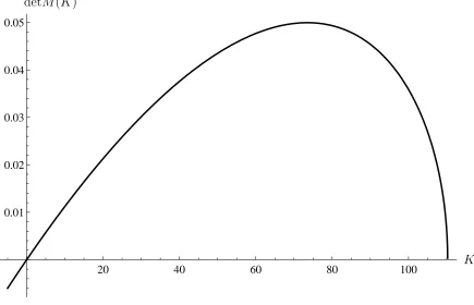
versus K for a given value of β. Using a range of values for K results in a plot with two unique roots that occur at K = 0 and K = 9β/2. Figure 2 illustrates how the determinant of a(Y) = ciYs subjected to equation (127) varies with K wheres is given by equation (125).
20 40 60 80 100 0.01
0.02 0.03 0.04 0.05
[image:35.595.116.551.205.485.2]K detM(K)
Figure 2: This is calculated usinga(Y) =ciYsalonside equations (125) and (127).
For Figure 2 when K = 0 the solution is a(Y) = c1Y +c2/Y2 which has two linearly independent eigenvectors that lead to a trivial solution where c1 =c2 = 0. The nontrivial solution occurs whenK = 9β/2 and has a solution represented by
a(Y) =c1Y− 1/2
+c2Y− 1/2
logY. (128)
leads toc1 =−c2/3 resulting in
a(Y) =c2
−1 3Y
−1/2
+Y−1/2 logY
. (129)
The angular expression b(Θ) which is given by equation (122) is solved for the boundary conditionsb(Θs = 1 andb′(Θs) = 0. This can be solved numerically and is a Legendre function of the first and second kinds. To determine c2 we apply the conservation of mass. The conservation of mass demands that
mref =mcurrent, (130)
whereρref =ρcurrentJ and J is the Jacobian is given by equation (74). This leads to
Vref = Z dV
current
J , (131)
which is solved numerically to give a value forc2 which is dependent on the opening angle Θop, the matching boundary condition Θsand the applied hoop (polar) stress
ˆ
pwhere ˆp=p/µ=ǫ.
12
Determining the collapse phase of the shell
for the radial component of the momentum
This section will focus on the collapse phase of the shell. To collapse the shell we
have to consider both the radial and angular components of the linear momentum
andρo is the density in the reference configuration,D/Dtis the material derivative andSis the first Piola Kirchoff stress tensor. Applying equation (132) to the radial component of the momentum gives
ρo
Dvr Dt
er =∇R·S, (133)
where vr = ∂r/∂t, vθ = r∂θ/∂t, vφ = 0 and the material derivative ([16], p354-p355) is written as
Dvr Dt =
∂vr ∂t +vr
∂vr ∂ri
+vθ r
∂vr ∂θi −
v2 θ
r . (134)
To nondimensionalise the material derivative represented by equation (158) we set
t=γˆt which results in
Dvr Dt =
RI γ2
∂2 y ∂ˆt2 +
∂y ∂ˆt
∂ ∂yi
∂y ∂tˆ
+ ∂θ
∂ˆt ∂ ∂θi
∂y
∂ˆt
−y
∂θ ∂tˆ
2!
, (135)
where the radial momentum component is given by
ρoR2I µoγ2
∂2 y ∂ˆt2 +
∂y ∂tˆ
∂ ∂yi
∂y ∂tˆ
+∂θ
∂ˆt ∂ ∂θi
∂y
∂ˆt
−y
∂θ ∂ˆt
2!
er =µr∇Y ·S,ˆ (136)
and ˆS is the nondimensionalised First Piola Kirchoff stress. Note that we have used a relative nondimensionalised shear modulus µr = µ/µo where µo = 20MPa in order to determine how varying the shear modulus influences the collapse time
to
∂2 y ∂ˆt2 +
∂y ∂tˆ
∂ ∂yi
∂y ∂ˆt
+∂θ
∂ˆt ∂ ∂θi
∂y
∂ˆt
−y
∂θ ∂ˆt
2!
er =µr∇Y ·S.ˆ (137)
To solve equation (137) we linearise where
y=Y +ǫj(Y,Θ,ˆt), (138)
and only the first term ∂2 y/∂ˆt2
is non-zero since all the remaining terms on the
left handside of equation (137) are second order. The right hand side of equation
(137) represented by µr∇Y ·S, is evaluated using the quasistatic solution for theˆ First Piola Kirchoff equation represented by equation (120) but with a caveat.
In equation (120) which denotes the deformation of the shell and is quasistatic,
the stresses can exhibit both a compressive and a stretching behaviour whereas in
the collapse phase the stresses are effectively all negative in nature and are thus
compressive only. To collapse the shell the signs of the relative terms in
equa-tion (120) are changed to represent a compression only behaviour. Applying the
linearisation represented by equation (138) to the compression modified equation
initially denoted by equation (120) results in
∂2 j ∂ˆt2 =µr
−4βj+ 4βY ∂j
∂Y −cot Θ ∂j ∂Θ−
∂2 j ∂Θ2 −2Y
2 β∂
2 j ∂Y2
. (139)
Using separation of variables where j(Y,Θ,ˆt) = A(Y)B(Θ)T(ˆt) and substituting into equation (139) gives
¨ T T =µr
−4β+ 4βY
A′
A
−cot Θ
B′
B
−
B′′
B
−2Y2β
A′′
A
which can be rewritten as
µr
−4β+ 4βY
A′
A
−2Y2 β
A′′
A
−ω2 =µr
B′′
B
+ cot Θ
B′
B
=Kµr. (141)
Equation (141) leads to two key equations
B′′+B′cot Θ−KB= 0, (142)
µr
−4β+ 4βY
A′
A
−2Y2 β
A′′
A
−K
−ω2
= 0, (143)
where K = 9β/2 which is obtained from the forward picture. To solve equations (142) and (143) we must consider the initial conditions for the collapse phase where
y=Y +ǫa(Y)b(Θ) =Y +ǫA(Y)B(Θ)T(0), (144) ∂j(Y,Θ,0)
∂ˆt = 0, (145)
which leads to
B(Θ) =b(Θ), (146)
A(Y) =a(Y)/T(0). (147)
Substituting equation (146) into equation (142) gives equation (122),b′′+b′cot Θ−
Kb = 0, from the forward (quasistatic) picture. Using equation (146) to solve equation (143) results in
µr
−4β+ 4βY
a′
a
−2Y2 β
a′′
a
−K
−ω2
From the forward picture expressed by equation (123)
−2Y2
βa′′ = 4βY a′ −(4β−K)a, (149)
which upon substituting into equation (148) leads to
ω2 =µr
8βY
a′
a
−8β
, (150)
wherea(Y) is given by equation (129). Solving equation (129) results in a general solution for a(Y) as a function of ˆpwhere ˆp=p/µ=ǫ which has the form
a(Y) =− pˆ 2√Y
−2c32 +c2logY
, (151)
wherec2 is evaluated numerically by applying the conservation of mass. Similarly
a′(Y)
a(Y) =
8−3 logY
2Y (3 logY −2), (152)
and
Y a′(Y)
a(Y) =
8−3 logY
2 (3 logY −2), (153)
where logY can be expanded aboutYI = 1 via a Taylor expansion series resulting in
Y a′(Y)
a(Y) ≈ −2− 9
4(Y −1). (154)
Substituting equation (154) into equation (150) for ω2
leads to
ω2
= 8βµr
−3− 9
4(Y −1)
where YI ≤Y ≤YO. Since YI = 1 andYO = 1.02 then the dependency of ω on Y is negligible.
13
Determining the collapse phase of the shell
for the polar component of the momentum
THis section will discuss the polar component during the collapse phase of the
shell. As well as there being a radial component of momentum there is also an
polar component of linear momentum. This is given by
ρo
Dvθ Dt
eθ =
1
R∇Θ·S, (156)
where
vθ =r ∂θ
∂t. (157)
The material derivative is given by ([16], p354-355)
Dvθ Dt =
∂vθ ∂t +vr
∂vθ ∂ri
+vθ r
∂vθ ∂θi
+vrvθ
r . (158)
and nondimensionalising where y=r/RI, Y =R/RI and t=γˆt leads to
Dvθ Dt =
RI γ2
∂ ∂tˆ
y∂θ
∂ˆt
+∂y ∂ˆt
∂ ∂yi
y∂θ
∂tˆ
+
∂θ ∂ˆt
∂ ∂θi
y∂θ
∂ˆt
+∂y ∂tˆ
∂θ ∂tˆ
. (159)
Linearising equation (159) where ǫ= ˆp using
results in
Dvθ Dt =
RIY γ2
ǫ∂
2 h ∂ˆt2
, (161)
since the second, third and fourth terms in equation (159) are higher order. The
nondimensionalised right hand side of equation (156) is given by
1
R∇Θ·S = µrµo RIY
∇Θ·Sˆ
, (162)
where ˆS represents the nondimensionalised First Piola Kirchoff stress and µr = µ/µo. Equating equations (161) and (162) results in the linearised, nondimen-sionalised polar component for the collapse phase of the linear momentum which
is
Y2 ǫ
∂2
h ∂tˆ2
eθ =µr∇Θ·Sˆ (163)
where γ =pρoR2I/µo. The nondimensionalised polar component of the First Pi-ola Kirchoff stress ˆS for the collapse phase of the shell is related to the quasistatic equation represented by equations (105) and (113). In the collapse phase each
contributing term in equation (113) will contribute a negative stress value which
represents a compression whilst the perturbation in the collapse phase is denoted
by ǫh(Θ,ˆt) rather than ǫg(Θ) for the quasistatic (forward) picture. Adjusting the signs in equation (113) such that all the terms are negative in magnitude and
applying the appropriate time evolving perturbation ǫh(Θ,ˆt) results in a nondi-mensionalised polar stress term given by
∇Θ·Sˆ=ǫµr −2β|h′′| −2β|h′cot Θ| −2βhcsc 2
Θ
which leads to the polar component of the linear momentum
Y2∂ 2
h
∂tˆ2 =µr −2β|h
′′| −2β|h′cot Θ| −2βhcsc2 Θ
. (165)
The polar component of the linear momentum represented by equation (165) is
solved numerically using finite differences. To solve equation (165) we require two
boundary and two initial conditions. The boundary condition at the opening angle
Θop is such that ˆτθθ Θop,ˆt
= 0 which leads to
h′+hcot Θ
op= 0, (166)
and at the matching boundary condition
h(Θs,ˆt) = 0. (167)
The initial conditions are
h(Θ,0) =g(Θ), (168)
and ∂h(Θ,0)
∂tˆ = 0, (169)
where equation (168) sets h(Θ,t) for the angular collapse phase at ˆˆ t= 0 equal to the forward picture g(Θ). This implies that there is no hysteresis in the collapse phase of the shell and that the forward and collapse paths are identical. This is a
14
Results for the deformation of an open shelled
spherical microbubble
1.005 1.010 1.015 1.020 0.02
0.04 0.06
Y
[image:44.595.114.547.165.446.2](4β+ 2)ǫfY + 2βǫ∂Y∂f
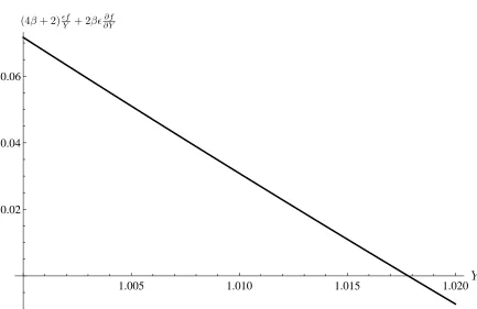
Figure 3: Graph of the radial terms in the polar hoop stress boundary condition for equation (112) for β = 24.5.
Figure 3 highlights how the magnitude of the radial terms in equation (112) vary
with Y and illustrates that the contribution of (4β + 2)ǫf /Y + 2βǫ∂f /∂Y to the nondimensionalised boundary condition is small. This justifies neglecting the
radial terms in equation (112) which results in an angular boundary condition that
0 .5 1 .0 1 .5 2 .0 2 .5 3 .0 0 .0 0 0 0 2
0 .0 0 0 0 4 0 .0 0 0 0 6 0 .0 0 0 0 8
[image:45.595.119.544.73.371.2]Θ ǫg(Θ)
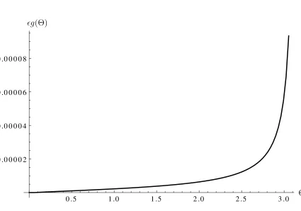
Figure 4: Graph of the angular perturbation for an open shell versus the refer-ence angle for a nondimensionalised hoop stress load of ˆp = 0.0002 where µ = 20MPa, ν = 0.49, β = 24.5 and an initial thickness of YO −YI = 0.02 for an opening angle of π−Θop = π/36 and a matching boundary condition given at Θs =π/45. This is calculated using equation (118).
Figure 4 illustrates how the angular perturbation, ǫg(θ), varies with the polar angle, Θ, in the reference configuration for a small opening angle π−Θop=π/36 and a nondimensionalised stress of ˆp = 0.0002. ǫg(θ), the perturbation of θ(Θ), is nonlinear and small in magnitude which is a consequence of the small opening
0 .5 1 .0 1 .5 2 .0 2 .5 3 .0 0 .5
1 .0 1 .5 2 .0 2 .5 3 .0
[image:46.595.120.517.83.368.2]Θ θ(Θ)
Figure 5: Graph of θ(Θ) for an open shell versus the reference angle, Θ, for a nondimensionalised stress load of ˆp = 0.0002 where µ = 20MPa, ν = 0.49, β = 24.5 and an initial thickness ofYO−YI = 0.02 for an opening angle ofπ−Θop= π/36 and a matching boundary condition at Θs = π/45. This is calculated using equation (118).
Figure 5 highlights how the polar angle, θ(Θ), in the current configuration varies with the polar angle in the reference configuration, Θ, for a small opening
angle given by π −Θop = π/36 and a matching boundary condition applied to the vicinity of the north pole at Θs = π/45. The polar angle θ(Θ) is linear in nature due to the small perturbation in ǫg(θ) which is a result of the small opening angle π−Θop. At the polar angular region of 0 ≤Θ≤π/45 the angular perturbation isǫg(θ) = 0 andθ(Θ) = Θ. This region represents the purely radially compressive region of the sphere where the matching boundary condition is applied
1 .0 0 5 1 .0 1 0 1 .0 1 5 1 .0 2 0 1 .0 4 0
1 .0 4 5 1 .0 5 0
[image:47.595.117.535.84.376.2]Y y(Y,Θop)
Figure 6: Graph of the nondimensionalised radius in the current configuration y(Y,Θ) versus the nondimensionalised radius in the reference configuration Y for a nondimensionalised stress load ˆp = 0.0002 where µ = 20MPa, ν = 0.49, β = 24.5 and an initial thickness ofYO−YI = 0.02 for an opening angle ofπ−Θop= π/36 and a matching boundary condition at Θs = π/45. This is calculated using equations (122) and (129).
0 .0 0 .5 1 .0 1 .5 2 .0 2 .5 3 .0 1 .0 1
1 .0 2 1 .0 3 1 .0 4 1 .0 5 1 .0 6
[image:48.595.118.538.83.384.2]Θ y(YO,Θ)
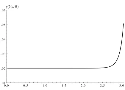
Figure 7: Graph of the nondimensionalised radius in the current configuration y(Y,Θ) versus Θ for a nondimensionalised stress load ˆp = 0.0002 where µ = 20MPa, ν = 0.49, β = 24.5 and an initial thickness of YO −YI = 0.02 for an opening angle ofπ−Θop=π/36 and a matching boundary condition at Θs=π/45. This is calculated using equations (122) and (129).
Figure 7 illustrates the nonlinear relationship between the radius y(YO,Θ) in the current configuration and the reference angle Θ for a small opening angle
0 .0 0 0 0 5 0 .0 0 0 1 0 0 .0 0 0 1 5 0 .0 0 0 2 0 0 .0 1 8 8
0 .0 1 9 0 0 .0 1 9 2 0 .0 1 9 4 0 .0 1 9 6 0 .0 1 9 8 0 .0 2 0 0
ˆ p
y(YO,Θop)−y(YI,Θop)
Figure 8: Graph of the Jacobian for a series of nondimensionalised stresses loads up to ˆp = 0.0002 where µ = 20MPa, ν = 0.49, β = 24.5 and an initial thickness ofYO−YI = 0.02 for an opening angle ofπ−Θop= π/36 and a matching boundary condition at Θs = π/45. This is calculated using equations (122) and (129).
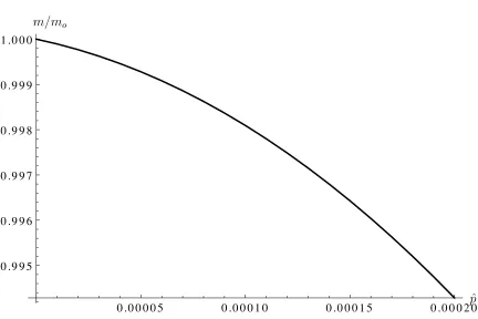
[image:49.595.132.517.96.326.2]0 .0 0 0 0 5 0 .0 0 0 1 0 0 .0 0 0 1 5 0 .0 0 0 2 0 0 .9 9 5
0 .9 9 6 0 .9 9 7 0 .9 9 8 0 .9 9 9 1 .0 0 0
[image:50.595.114.546.85.373.2]ˆ p m/mo
Figure 9: Graph of the normalised mass m/mo for a series of nondimension-alised stresses loads up to ˆp = 0.0002 where µ = 20MPa, ν = 0.49, β = 24.5 and an initial thickness ofYO−YI = 0.02 for an opening angle ofπ−Θop= π/36 and a matching boundary condition at Θs = π/45. This is calculated using equations (74), (122) and (129).
Figure 9 illustrates how the normalised mass of a stressed shell evolves
(for-ward picture) over a range of nondimensionalised stresses ˆp up to ˆp= 0.0002 and highlights that the error in mass conservation is ≈0.6%.
15
Results for the collapse phase of an open shelled
spherical microbubble
0.000 0.002 0.004 0.006 0.008 0.010 0.0000
0.00002 0.00004 0.00006 0.00008 0.0001
[image:51.595.113.547.79.373.2]ˆ t ǫh(Θop,t)ˆ
Figure 10: Graph of the polar angle perturbation h(Θop,t) versus the nondimen-ˆ sionalised time forµ = 20MPa, ν = 0.49, β = 24.5, an initial thickness ofYO− YI = 0.02, an opening angle of π−Θop=π/36 and a matching boundary condition at Θs = π/45. This is calculated using equations (165), (166), (167), (168) and (169).
Figure 10 shows how the polar angle perturbation ǫh(Θ,ˆt) varies with the nondimensionalised time as the stressed shell collapses back to its original stress
free configuration when ∇θ·τ = 0. Figure 10 illustrates that the nonlinear trend is a sinusoidal function described by equation (165) describing simple harmonic
motion. This is a consequence of the negative stress (compressive) terms which
40 60 80 100 0.005
0.006 0.007 0.008 0.009
µ ˆ
[image:52.595.114.546.74.383.2]t∗
Figure 11: Graph of the nondimensionalised collapse time for the collapse phase of the shell versus a range of shear modulus values for ν = 0.49, β = 24.5, an initial thickness ofYO−YI = 0.02, an opening angle ofπ−Θop =π/36 and a matching boundary condition at Θs =π/45. This is calculated using equations (165), (166), (167), (168) and (169).
Figure 11 illustrates how the collapse time decreases nonlinearly with an
in-creasing shear modulus. A smaller shear modulus experiences a larger
displace-ment due its lower stiffness. Larger displacedisplace-ments (for a given fixed stress p) will take longer to collapse back to their initial stress free position. Therefore as the
shear modulus increases there is a reduction in the shell’s displacement which
0.491 0.492 0.493 0.494 0.495 0.0070
0.0075 0.0080 0.0085 0.0090 0.0095
ν ˆ
[image:53.595.114.549.78.377.2]t∗
Figure 12: Graph of the nondimensionalised collapse time versus a range of Poisson ratios for µ = 20MPa, an opening angle of π − Θop = π/36 and a matching boundary condition at Θs=π/45. This is calculated using equations (165), (166), (167), (168) and (169).
Figure 12 shows that when the Poisson ratio, ν, increases then the collapse time of the shell decreases, resulting in a faster collapse time. This relationship is
effectively linear in nature and is modelled over the typical range of Poisson values
for soft tissue, namely ν = 0.49 to 0.495. This trend arises because smaller Pois-son ratios experience larger displacements which results in longer, slower collapse
0.02 0.04 0.06 0.08 0.10 0.000
0.002 0.004 0.006 0.008 0.010 0.012 0.014
YO−YI
[image:54.595.114.553.76.386.2]ˆ t∗
Figure 13: Graph of the nondimensionalised collapse time ˆt∗ versus a range of
nondimensionalised stress free shell thicknesses ranging fromYO−YI = 0.02 to 0.10 for µ = 20MPa, ν = 0.49, β = 24.5, an opening angle of π −Θop = π/36 and a matching boundary condition at Θs =π/45. This is calculated using equations (165), (166), (167), (168) and (169).
Figure 13 highlights how the collapse time slightly increases linearly with
vary-ing shell thicknesses (reference configuration thickness). Generally thinner shell
require a lower applied stress to create a particular angular displacement, hence
the resulting tensions are lower, and a higher collapse time results. However,
care-ful analysis of equation (165) reveals a dependency on Y2
. Thus as the thickness
of the shell increases the acceleration downwards during the collapse phase of the
shell is reduced by a factor of 1/Y2
0 .0 0 2 0 .0 0 4 0 .0 0 6 0 .0 0 8 0 .9 9 4 5
0 .9 9 5 0 0 .9 9 5 5 0 .9 9 6 0 0 .9 9 6 5 0 .9 9 7 0 0 .9 9 7 5
[image:55.595.114.536.103.375.2]ˆ t m/mo
Figure 14: Graph of the normalised mass m/mo of a stressed, collapsing shell where µ= 20MPa, ν = 0.49, β = 24.5 and an initial thickness ofYO−YI = 0.02 for an opening angle of π−Θop = π/36 and a matching boundary condition at Θs =π/45. This is calculated using equations (165) to (169).
Figure 14 illustrates that the normalised mass of a collapsing shell versus the
nondimensionalised time is nonlinear in nature. The error in mass conservation is
0.00 0.01 0.02 0.03 0.04 0.05 0.06 0.07 0.00
0.01 0.02 0.03 0.04
[image:56.595.112.546.80.388.2]ˆ t ǫj(YI,Θop,t)ˆ
Figure 15: Graph of the radial perturbationj(YI,Θop,ˆt) versus the nondimension-alised time forµ= 20MPa, ν = 0.49, β = 24.5, an initial thickness ofYO−YI = 0.02, an opening angle of π−Θop=π/36 and a matching boundary condition at Θs =π/45. This is calculated using equations (142), (144), (145), (151) and (155).
Figure 15 shows how the radial perturbationǫj(YI,Θop,ˆt) varies with the nondi-mensionalised time as the stressed shell collapses back to its original stress free
configuration when ∇y ·τ = 0. Figure 15 illustrates that the nonlinear trend is a sinusoidal function that is characterised as simple harmonic motion. This is a
consequence of the negative stress (compressive) terms which cause the stressed
shell to collapse to its original stress free configuration. Note that the radial
col-lapse time is ˆt∗ ≈ 0.09 and is slower than the polar angular collapse. We would
imations that have been made when performing the linearisation process. For the
radial displacement the collapse times and their dependency on varying material
parameters display similar characteristic trends as Figures 11, 12 and 13.
16
Experimental v theoretical results
This section compares the theoretical model with published experimental results.
The M¨uller experiment [7] illustrates how the collapsing shelled millibubble’s
dis-placement varies linearly with time. This linear relationship allows us to
extrap-olate M¨uller’s experimental results and also supports the use of linearisation for
the analytical model. The theoretical model for the open shelled collapse was
compared to the M¨uller experiment [7]. The shear modulus of the shell was taken
as µ = 20MPa with a density of ρ = 1100kgm−3
[17]. A 4.5mm stressed shelled
millibubble of thickness 1460nm with a Poisson ratio ofν= 0.49 has a theoretical collapse time oft∗ = 3.2×10⁻⁷
s whereas the experimental result from M¨uller was
found to be t∗ = 7.4×10⁻⁷
s. There are various reasons as to why the theoretical
model’s collapse time differs from the experimentally observed value. The material
parameters used for the theoretical model may not exactly match the
experimen-tal values in [7]. The strain energy density function used in this study may not
accurately describe the smectic A dynamics.
17
Conclusion
This study has focussed on how the material parameters such as the shear
modu-lus, Poisson’s ratio and the shells equilibrium (stress free) thickness influences the
the stress free configuration with a polar hoop stress being applied to deform both
radially and angularly the open sphere. The Cauchy polar hoop stress was then set
to zero causing the stressed shell to collapse to its stress free configuration. This
collapse phase was timed by applying the conservation of mass and energy and
by assuming that there was no viscosity or viscoelastic effects in the model that
would lead to hysteresis. A typical shell with an opening angle ofπ−Θop=π/36, a nondimensionalised stress free thickness ofYO−YI = 0.02, a nondimensionalised shear modulus ofµ= 20MPa and a typical soft tissue Poisson ratio ofν = 0.49 has a nondimensionalised collapse time of ˆt∗ = 0.0096. As the shear modulus increases
the collapse time decreases in a nonlinear manner. Thicker shells have slightly
longer collapse times which is a consequence of the shells possessing a smaller
ac-celeration towards their equilibrium position. Smaller Poisson ratios have longer,
slower collapse times with the relationship between the collapse time and Poisson’s
ratio being effectively linear in nature. The theoretical model compares well with
published experimental results for smectic A millibubbles [7]. A theoretical
col-lapse time oft∗ = 3.2×10⁻⁷
s was determined whereas the published experimental
result from M¨uller was found to be t∗ = 7.4×10⁻⁷ s.
References
[1] E. Stride and N. Saffari. Microbubble ultrasound contrast agents: a review.
Proceedings of the Institution of Mechanical Engineers Part H, 217:429–447,
2003.
[2] J. McLaughlan, N. Ingram, P.R. Smith, S. Harput, P.L. Coletta, S. Evans,