Segment-Based Predominant Learning Swarm
Optimizer for Large-Scale Optimization
Qiang Yang, Student Member, IEEE, Wei-Neng Chen, Member, IEEE, Tianlong Gu, Huaxiang Zhang,
Jeremiah D. Deng, Member, IEEE, Yun Li, Member, IEEE, and Jun Zhang, Senior Member, IEEE
Abstract—Large-scale optimization has become a significant yet
challenging area in evolutionary computation. To solve this problem, this paper proposes a novel segment-based predominant learning swarm optimizer (SPLSO) swarm optimizer through letting sev-eral predominant particles guide the learning of a particle. First, a segment-based learning strategy is proposed to randomly divide the whole dimensions into segments. During update, variables in different segments are evolved by learning from different exemplars while the ones in the same segment are evolved by the same exemplar. Second, to accelerate search speed and enhance search diversity, a predominant learning strategy is also proposed, which lets several predominant particles guide the update of a particle with each pre-dominant particle responsible for one segment of dimensions. By combining these two learning strategies together, SPLSO evolves all dimensions simultaneously and possesses competitive exploration and exploitation abilities. Extensive experiments are conducted on two large-scale benchmark function sets to investigate the influ-ence of each algorithmic component and comparisons with several state-of-the-art meta-heuristic algorithms dealing with large-scale problems demonstrate the competitive efficiency and effectiveness of the proposed optimizer. Further the scalability of the optimizer to solve problems with dimensionality up to 2000 is also verified.
Index Terms—Global numerical optimization, large-scale
opti-mization, particle swarm optimization (PSO), segment-based predominant learning swarm optimizer (SPLSO).
Manuscript received March 22, 2016; revised July 4, 2016; accepted October 3, 2016. Date of publication October 24, 2016; date of cur-rent version August 16, 2017. This work was supported in part by the National Natural Science Foundation of China under Grant 61622206, Grant 61379061, and Grant 61332002, in part by the Natural Science Foundation of Guangdong under Grant 2015A030306024, and in part by the Guangdong Special Support Program under Grant 2014TQ01X550. This paper was rec-ommended by Associate Editor Y. Tan. (Corresponding authors: Wei-Neng
Chen; Jun Zhang.)
Q. Yang is with the School of Computer Science and Engineering, South China University of Technology, Guangzhou 51006, China, and also with the School of Data and Computer Science, Sun Yat-sen University, Guangzhou 510006, China.
W.-N. Chen and J. Zhang are with the School of Computer Science and Engineering, South China University of Technology, Guangzhou 51006, China (e-mail:[email protected];[email protected]).
T. Gu is with the School of Computer Science and Engineering, Guilin University of Electronic Technology, Guilin 541004, China.
H. Zhang is with the School of Information Science and Engineering, Shandong Normal University, Jinan 250014, China.
J. D. Deng is with the Department of Information Science, University of Otago, Dunedin 9054, New Zealand.
Y. Li is with the School of Computer Science and Network Security, Dongguan University of Technology, Dongguan 523808, China.
This paper has supplementary downloadable multimedia material available athttp://ieeexplore.ieee.orgprovided by the authors. This includes a PDF file which contains additional tables and figures not included within the paper itself. The total size of the file is 1.048 MB.
Color versions of one or more of the figures in this paper are available online athttp://ieeexplore.ieee.org.
Digital Object Identifier 10.1109/TCYB.2016.2616170
I. INTRODUCTION
E
VOLUTIONARY optimization has witnessed great suc-cess in many optimization problems [1]–[6] and has been applied to many real-world applications [7]–[12] in recent years. Owing to its easiness of understanding and implementation, a lot of attention has been devoted to evolutionary algorithm (EA) researches and subsequently many different EAs have been developed, such as parti-cle swarm optimization (PSO) algorithms [13]–[21], dif-ferential evolution (DE) algorithms [22], [23], ant colony optimization (ACO) algorithms [24], [25], estimation of dis-tribution algorithms [26], [27], firefly algorithms [5], [28], etc. In particular, since PSO was first developed by Eberhart and Kennedy [17], [18], an ocean of PSO variants have been proposed, such as clustering-based PSO [29], scat-ter learning PSO [30], adaptive PSO [13], [31], comprehensive learning PSO (CLPSO) [32], and bare bone PSO [14], [15].Although traditional EAs have shown their excellent abil-ities and feasibilabil-ities in low-dimensional space (less than 100-D), their performance would deteriorate dramatically when it comes to high-dimensional space [33], which is usually called “the curse of dimensionality.” Such inferior performance can be attributed to the drastic and exponential increase of the search space with the growing dimension-ality, forming large and massive local regions that easily cause the search process to stagnate into local optima and result in premature convergence for traditional EAs [33], [34]. Therefore, to tackle large-scale problems (more than 500-D), new evolution or learning strategies need to come up for EAs to escape from being trapped at local optima.
In recent years, works on large-scale optimization problems mainly followed two approaches.
1) Proposing cooperative coevolution (CC) strategies, which mainly concentrate on decomposing dimensions into groups and evolve each dimension group separately. 2) Proposing new learning strategies for traditional EAs evolving all dimensions together, which have great power in enhancing population diversity.
CC-based algorithms adopt the divide-and-conquer strat-egy to decompose high-dimensional problems into smaller subproblems. Since Potter [35] proposed such a promis-ing CC framework, researchers have developed many variants by utilizing different EAs (CCEAs) for large-scale optimization, such as cooperative coevolutionary genetic algorithm [36]–[38], cooperative coevolutionary PSO (CCPSO) [16], [33], and cooperative coevolutionary
DE (DECC) [39]–[43]. Currently, the research of CCEAs mainly focuses on proposing a good decomposition strat-egy, which aims to group independent variables into different groups and simultaneously group interdependent variables into the same group. So far, there are four kinds of decompo-sition strategies [41]: 1) random grouping [40], [42], [43], 2) perturbation grouping [44], [45], 3) interaction adaptation grouping [41], [46], [47], 4) model building grouping [48]. Even though CCEAs are promising for large-scale problems, they encounter three limitations.
1) CCEAs usually need a considerable number of fitness evaluations to obtain satisfactory solutions due to evolv-ing each subproblem separately, especially when the number of dimension groups is large.
2) A good decomposer has to detect dependency among variables by using a certain number of fitness evalua-tions [41], [45], at the sacrifice of fitness evaluations used for evolving.
3) When the fitness landscape of the problem becomes more and more complicated, e.g., the dynamic variable dependency in piecewise functions, the current dimen-sion grouping strategies embedded in CCEAs would lose their efficiency in detecting the dependency among variables.
The above limitations restrict the wide application of CCEAs when faced with limited resources, such as the limited number of fitness evaluations.
To relieve the above dilemma in CCEAs, from another aspect, researchers attempt to develop new learning strategies for traditional EAs to enhance the diversity, which contribute to promoting the chances of escaping from local optima for the population. Such new learning strategies are usually embedded in the update of particles, which is in the form of learn-ing from potential particles. Along this way, [49]–[54] show their feasibility and efficiency. CMA-ES [49] equips the evo-lution strategy (ES) with self-adaptive mutation parameters through computing a covariance matrix and correlated step sizes, which takes O(D2)(D is the dimension size), while sep-CMA-ES [50] is a simple modification of CMA-ES, which reduces the update of the whole covariance matrix to the update of its diagonal components. Recently, a multiswarm PSO based on feedback evolution (FBE) [54] and a com-petitive swarm optimizer (CSO) [53] were brought up with competitive learning strategies based on pairwise competition between particles, which will be detailed in the next section.
Though these proposed new learning strategies have shown feasibility on large-scale optimization, early-stagnation is still a main challenge for EAs. To prevent from being trapped in local optima, specific diversity enhancement strategies have to be designed to further improve search diversity.
In order to circumvent the dilemmas that CCEAs [16], [35], [41], [42], [45] and traditional EAs [50], [53], [54] are con-fronted with, this paper intends to take advantage of these two kinds of approaches and develop a novel segment-based predominant learning (SPL) swarm optimizer (SPLSO). More specifically, This paper contains the following components.
1) Segment-Based Learning (SL): Inspired from the facts that exemplars made up by combining dimensions from
different exemplars would lead to potentially better directions in orthogonal learning PSO (OLPSO) [55] and that learning from different exemplars can greatly enhance the diversity in CLPSO [32], an SL strat-egy is proposed to learn segments of potentially useful information from different exemplars. First, SL ran-domly divides dimensions into segments. Then, for each segment of a particle, SL lets one exemplar guide the update of this part. Together, SL allows several exemplars to simultaneously guide the learning of one particle. Through this, on one hand the potentially ben-eficial evolutionary information embedded in different exemplars may be gathered and learned by particles; on the other hand, the potentially useful information in different dimensions of an exemplar may be pre-served and gathered together. In this way, SL performs a new way of coevolution for different dimension segments.
2) SPL: Inspired by the competitive learning strategy in CSO [53], this paper further couples SL with a predom-inant learning strategy (PL), leading to a novel learning strategy called “SPL.” SPL divides particles into rela-tively good ones and poor ones. Then each poor particle performs SL to learn from different good ones. That is, each dimension segment of this particle is updated by randomly selecting a relatively good particle as its exemplar. In this way, SPL not only potentially intro-duces high diversity as all predominant particles can potentially become exemplars, but also enables an effec-tive interaction among different dimension segments of predominant particles, which may contribute to a fast convergence speed.
To verify the proposed SPLSO, a series of experiments are conducted on widely used CEC’2010 and CEC’2013 large-scale benchmark functions. The experimental results in comparison to state-of-the-art algorithms coping with large-scale optimization demonstrate the competitive efficiency and effectiveness of SPLSO. In addition, the comparison results between SPLSO and CSO [53] on 20 CEC’2010 prob-lems with 2000-D further substantiate the good scalability of SPLSO to higher dimensionality.
The remainder of this paper is organized as follows. SectionIIintroduces the classical PSO and its variants in deal-ing with large-scale optimization. Then, SPLSO is stated in detail in SectionIII. In SectionIV, experiments are conducted to verify the effectiveness of SPLSO in comparison with five state-of-the-art algorithms. At last, Section V concludes this paper.
II. RELATEDWORK
Without loss of generality, a D-dimensional minimization problem considered in this paper can be formulated as
min f(x),x∈RD (1)
A. PSO
PSO [17], [18] simulates the swarm behaviors of social ani-mals such as bird flocking, and is modeled on an abstract framework of “collective intelligence.” Usually, particles in a swarm represent points in the D-dimensional search space and two attributes, namely position and velocity, are assigned to each particle. Suppose the position and velocity of the swarm are denoted as X and V, with the ith particle identified as
Xi and Vi, respectively, and then the update of these two attributes are
vdi ←wvdi +c1r1
pbestdi −xdi
+c2r2
gbestd−xid
(2)
xdi ←xdi +vdi (3)
where Xi=[x1i, . . . ,xdi, . . . ,xDi ] is the position of the ith par-ticle, and Vi = [v1i, . . . ,vdi, . . . ,vDi ] is its velocity, D is the dimension size, pbesti = [pbest1i, . . . ,pbestdi, . . . ,pbestDi ] is
the personal best position of the ith particle, and gbest = [gbest1, . . . ,gbestd, . . . ,gbestD] is the global best position of the whole swarm. Among parameters, c1and c2are two accel-eration coefficients [17], r1 and r2 are uniformly randomized within [0,1], and w is termed as the inertia weight [56]. Kennedy and Eberhart [18] referred to the second and the third part in the right of (2) as the cognitive component and the social component, respectively.
An outstanding characteristic of PSO is the fast conver-gent behavior and inherent adaptability. Theoretical analysis of PSO [57] has shown that particles in a swarm can keep a balance between exploration and exploitation. However, due to the strong influence of the global best position gbest on the convergence speed [33], premature convergence remains a major issue in PSO. Thus, some researchers proposed to utilize the neighbor best position [17], [57], [58] to replace the global best position in updating the velocity of each particle.
Further, some researchers even put forward strategies to construct new exemplars to lead the learning direction. Along this line, two influential representatives are OLPSO [55] and CLPSO [32]. OLPSO constructs a new exemplar by combining dimensions from the personal best position and the neigh-bor best position of each particle via orthogonal experimental design (OED). As for the construction of the new exemplar in CLPSO, with respect to each dimension of the exemplar, two personal best positions are first randomly selected and the value of the dimension from the better one fills in the corre-sponding dimension of the new exemplar. Thus, the velocity update in CLPSO is formulated as
vdi ←wvdi +crdi
pbestdf i(d)−x
d i
(4)
where fi =[fi(1), . . . ,fi(d), . . . ,fi(D)] defines a series of pbest
of different particles that the ith particle should follow, rdi is randomly generated within [0, 1], and w and c are the inertia weight and the acceleration coefficient as in (2), respec-tively. Both OLPSO and CLPSO show great efficiency in low-dimensional space; however, they are not suitable for large-scale problems because, on one hand OLPSO needs a lot of fitness evaluations in OED to seek the poten-tially useful combination of dimensions, which is impractical
for large-scale problems; on the other hand, CLPSO con-verges considerably slowly owing to the construction strategy that each dimension of the new exemplar corresponds to a randomly selected personal best position. Nevertheless, the way to learn from different exemplars behind these two optimizers inspires us to propose the SL strategy in this paper.
B. PSO Variants for Large-Scale Optimization
When it comes to high-dimensional space (larger than 500-D), the classical PSO [17], [18] and most of its vari-ants [13], [31], [32], [55] will lose their effectiveness due to the drastic and exponential enlargement of the search space when the dimensionality grows. That massive local optima exist in the high-dimensional space is another challenge, leading to easily being trapped into local areas for EAs [53].
As for the first approach to large-scale optimization, some works have been done to combine CC framework [35] with the classical PSO and its representative variants, resulting in CCPSO. CCPSO-SK [33] randomly divides the whole
dimensions into K groups with each group containing D/K
dimensions. Then for each dimension group, the classical PSO is applied to optimize the subspace, while dimensions in the other groups are fixed to the corresponding part of the global best solution gbest. Through this cooperation among dimension groups, CCPSO-SK is promising to solve
large-scale optimization. In CCPSO-HK [33], the classical PSO and
CCPSO-SKare used in an alternating manner, with CCPSO-SK
executed for one iteration, followed by the classical PSO in the next generation. While in CCPSO2, Li and Yao [16] designed a decomposer pool consisting of different group sizes, and the algorithm will randomly select a group size from the pool every time gbest is not improved. In addition, the offspring of each parent for each dimension group is randomly sampled around the personal best position or the neighbor best position according to the Cauchy [59] or Gaussian distributions [14].
Currently, the research of CCEAs including CCPSO [16], [33] mainly focuses on proposing good decomposers to divide dimensions into groups, which is the key of the CC framework. So far, CC with variable interaction learning [45] and differential grouping (DG) [41] are the most representative ones, which can potentially detect the dependency among variables. While CCEAs are promising for solving high-dimensional problems, they pay huge cost in fitness evaluations owing to optimizing each subcompo-nent individually, especially when the number of groups is large.
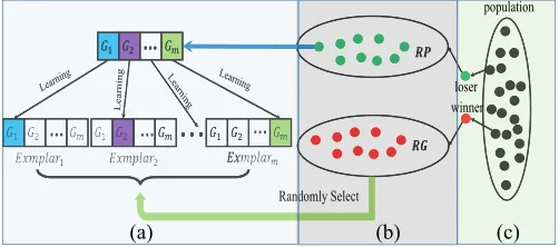
(a) (b) (c)
Fig. 1. Visual framework of SPLSO containing three parts. (a) SL. (b) PL. (c) Particle competition.
only the loser is updated, while the winner directly enters the next generation. The update process of the loser is formulated as
vdl ←r1vdl +r2
xdw−xdl
+φr3
xd−xdl
(5)
xdl ←xdl +vdl (6) where Vl = [v1l, . . . ,vdl, . . . ,vDl ] is the velocity of the loser,
Xl = [x1l, . . . ,xdl, . . . ,xDl ] and Xw = [x1w, . . . ,xdw, . . . ,xDw]
are the positions of the loser and the winner, respectively,
x =[x1, . . . ,xd, . . . ,xD] is the mean position of the current
population, r1–r3 are three uniformly random variables rang-ing within [0,1], andφis a parameter controlling the influence of x. In this formula, the second part of (5) enforces the loser move toward the winner, possibly resulting in a tendency to approach to the global optima, while the third part may poten-tially make the particle dragged away from the local area. Such randomized pairwise competition can greatly enhance the diversity of the population, which is very beneficial for large-scale optimization.
However, we find that during one competition, the loser learns deterministically only from the winning counterpart. As a consequence, the learning ability of the loser is restricted. Such an observation, along with considerations elaborated in Section II-A, motivates us to propose the SPL swarm optimizer (SPLSO).
III. SEGMENT-BASEDPREDOMINANT LEARNINGSWARMOPTIMIZER
SPLSO intends to gather the potentially useful evolution-ary information, which is concealed in different exemplars, to guide the learning of each particle, so that both diversity and convergence can be promoted to address large-scale optimiza-tion problems. The whole framework of SPLSO is shown in Fig.1. First, an SL method displayed in Fig.1(a) is introduced in SPLSO, which draws lessons from two representative PSO variants (OLPSO [55] and CLPSO [32]). Second, to get a fast convergence speed, a PL strategy, as shown in Fig.1(b) accom-panies SL, resulting in an SPL strategy. In addition, to deal with the difficulty in determining the optimal number of seg-ments in SPL, a segment number pool consisting of different numbers of segments is designed. It is noticed that this paper contributes to the second approach to large-scale optimization.
The detailed techniques adopted in SPLSO are presented as follows.
A. Segment-Based Learning
From the excellent performance of OLPSO [55] and CLPSO [32] in low-dimensional space, we find that learning from different exemplars through combining dimensions can potentially offer good directions for particles. However, origi-nally both OLPSO and CLPSO are not suitable for large-scale optimization, because, for one thing, they all learn informa-tion for each dimension separately; for another, OLPSO costs a lot of fitness evaluations to seek the best combination of dimensions, while CLPSO proceeds to the global optima very slowly. Such observation affords the inspiration for the SL method we are proposing.
As illustrated in Fig.1(a), SL first divides all dimensions of one particle into m disjoint segments with each segment con-taining D/m dimensions,1 i.e., G = {G
1, . . . ,Gj, . . . ,Gm},
where Gj is the jth dimension segment containing a set
of variables. Then, the position Xi = [x1i, . . . ,xid, . . . ,xDi ]
of the ith particle is accordingly divided into m subvectors
XG1
i , . . . ,X
Gj
i , . . . ,X
Gm
i , where X
Gj
i is a vector of variables
from Xi that belong to the jth segment. Likewise, the
veloc-ity Vi = [v1i, . . . ,vdi, . . . ,vDi ] is divided into m subvectors
VG1 i ,V
G2
i , . . . ,V
Gm
i , as well. Subsequently, during the update
of velocity and position in SPLSO, SL can be characterized by the following three rules.
1) For the dimensions in segment Gj of the ith
parti-cle, the particle’s corresponding velocity subvector VGji and position subvector XGi j are updated as a whole by learning from the same exemplar.
2) For different dimension segments, different exemplars can be used to update different velocity and position subvectors.
3) During one generation, though the number of segments is fixed, the random segmentation on dimensions is exe-cuted for each particle to be updated, which means that the components of each counterpart segment are differ-ent for differdiffer-ent particles, namely the segmdiffer-ent Gjof the
ith particle may be different from that of the kth particle.
Compared with traditional learning strategies in PSO vari-ants, especially in OLPSO [55] and CLPSO [32], SL can potentially increase the probability of preserving the useful information embedded in one exemplar together according to rule 1. Rule 2 allows particles to learn from differ-ent exemplars, which can potdiffer-entially collect useful evolution information existing in different exemplars as indicated in OLPSO [55] and CLPSO [32]. Such learning behavior may promote the diversity to some extent. As for rule 3, it is an auxiliary to rules 1 and 2, because for different exemplars, the segments of potentially useful information may be differ-ent. On one hand, it can enhance the probability to preserve the potentially beneficial information in different exemplars together; on the other hand, such behavior may improve the diversity to some extent.
Remark: Using the above three rules, SL also enforces
a special kind of coevolution among the dimension seg-ments, which differs from the CC framework significantly. It should be noted that although both SL and CCEAs need to divide the dimensions into disjoint parts, they work in very different ways. CCEAs consider each dimension group as a separated subproblem and evolve each subproblem indi-vidually. Thus, interdependent variables should be gathered into the same group while independent variables should be put into different groups according to variable dependency. However, SL mainly aims to let each relatively poor particle learn a segment of potentially useful information from dif-ferent predominant exemplars, so that the useful evolutionary information in different exemplars can potentially be gathered and learned by particles. Thus, this strategy is to increase the probability of gathering the potentially useful informa-tion in different predominant exemplars together, but not to increase the probability of putting interdependent variables into the same group as in CCEAs. In high-dimensional prob-lems, it is likely that in SL, a segment of variables from one predominant exemplar containing beneficial evolutionary information includes interdependent and independent variables simultaneously. Obviously, this is totally different from or even violates the aim of the decomposers in CCEAs. Thus, it is likely that the decomposition methods in CCEAs are not suit-able for the proposed SL. In addition, instead of treating each segment as a subproblem and evolving each group individually in CCEAs, SL treats all dimensions as a whole and evolves them simultaneously.
In a word, the difference both in dividing dimensions into segments and in evolving variables between SL and CCEAs makes SPLSO very different from CCEAs. Since currently, no effective indicator exists to measure the usefulness of one dimension of an exemplar, we just adopt random segmentation in this paper to divide the dimensions of each particle into m segments. Through this random recombination, on one hand, the potentially useful information in different dimensions of an exemplar may be simultaneously gathered; on the other hand, the potentially useful information in different exemplars may be gathered together with a probability.
B. Segment-Based Predominant Learning
Following SL, a crucial issue is how to select different exemplars for different dimension segments. To solve this issue, we further put forward the PL strategy to cooperate with SL, leading to SPL.
In general, diversity enhancement is accompanied with slow convergence, which is another concern for traditional EAs [13], [14], [30], [53]. In nature, it is common that a particle follows the experience from those which are better than itself. Enlightened by such an idea, we propose the PL strategy.
First, the whole swarm is organized into pairs randomly and the particles in each pair are compared with each other. When making pairwise comparisons between particles, usually one particle is dominated by the other. Therefore, two separated sets, the relatively good particles RG and the relatively poor
ones RP, are generated with the better one entering RG while the worse one belonging to RP as shown in Fig.1(b) and (c). Generally speaking, particles in RG usually hold more poten-tially useful information. Therefore, particles in RP should update their positions through utilizing beneficial information from particles in RG as much as possible. This is the main idea of PL.
Combining SL and PL together, SPL tries to make one poor particle learn segments of useful information from different good particles, which can be formulated as follows:
VGi
RPj ←r1V Gi RPj +r2
XGi
RGg(j,i) −X
Gi RPj
+φr3
ˆ
xGi−XGiRP
j
(7)
XGiRPj ←XGiRPj+VGiRPj (8)
where RPj denotes the jth relatively poor particle in RP, G=
{G1, . . . ,Gi, . . . ,Gm}is the dimension segments with totally
m segments, g(j,i)indicates the index of the relatively good particle in RG that the jth relatively poor particle will learn from for the segment Gi, x is the weighted mean position ofˆ
the whole population, r1–r3are three random variables ranging within [0,1], and φ is the controlling parameter in charge of the influence ofx.ˆ
The first part in the right of (7) is similar to the inertia term in PSO (2), which is mainly responsible for the sta-bility of the search process. The second part can also be called the cognitive component like in PSO. Instead of learning from pbest, SPLSO learns from all potentially good parti-cles through dimension segments. This part offers the chances of providing particles with better directions, which may con-tribute to fast convergence. As for the third part, we can also name it as the social component as in PSO. This part takes the responsibility to drag the particles away from local optimum areas. Instead of using mean position x in CSO [53], SPLSO shares the social knowledge through the weighted mean posi-tion of the whole swarm xˆ =[ˆx1, . . . ,xˆd, . . . ,xˆD], which is defined as
ˆ
xd=
NP
i=1
fit(Xi)
NP
j=1fit
Xj
xdi (9)
where NP is the population size, and fit(·) is the fitness function, defined as the function to be optimized in this paper. For simplicity, the fitness values of particles are utilized to determine the weight of each particle. To deal with problems with negative fitness values, we adjust (9) as follows:
ˆ
xd=
NP
i=1
fit(Xi)+ |fitmin| +η
NP
j=1
fitXj
+ |fitmin| +η
xdi (10) where fitminis the minimum fitness value of the swarm andη is a small positive value used to avoid a zero denominator.
In (9) or (10),x puts more emphasis on inferior particles,ˆ
which may be beneficial for dragging particles away from local optimum areas. In fact, this weighted mean positionx is func-ˆ
on inferior particles, which possess more powerful exploration ability than superior ones. On the other hand, in large-scale problems, usually, many local optima exist. Thus, superior par-ticles may easily fall into local areas, leading to premature convergence. However, this situation can be alleviated and the chances of escaping from local traps can be enhanced through putting more weight on inferior particles. In SectionIV-B2, the influence of x will be investigated through comparing againstˆ x and the experimental result favors x.ˆ
Note that SPL only operates on particles in RP, indicating that only half of the swarm is updated in each generation.
Though (7) has characterized SPL, some detailed techniques have to be mentioned here.
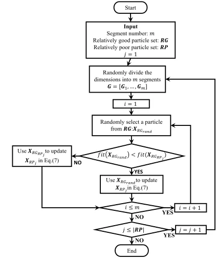
1) During each generation, the relatively good particle set
RG and the relatively poor particle set RP are
gen-erated through random pairwise comparison with RG associated with the better ones and RP related to the worse ones.
2) During the update of poor particles, for each segment
Gi of the jth poor particle XRPj, a random good parti-cle XRGrand is selected from RG, and then we compare
the fitness of this randomized good particle fit(XRGrand)
with that of the poor particle’s corresponding dominator fit(XRGRPj). If fit(XRGrand) <fit(XRGRPj), we will update
the poor particle using the randomized good particle
XRGrand in (7), otherwise, we will use its corresponding
dominator XRGRPj to update this particle.
3) For each poor particle in RP, the random segmentation on dimensions is conducted, resulting in m segments
G= {G1, . . . ,Gi, . . . ,Gm}. Note that for different poor
particles, the partition may be different, but the number of segments is the same.
First, the random pairwise comparison is adopted in tech-nique 1 because such randomness can allow some poor particles to survive, which may contribute to the promotion of diversity. However, this also may result in that some rel-atively good particles in RG may be dominated by some relatively poor ones in RP. Thus, not all relatively good par-ticles are valuable for the relatively poor ones. Generally speaking, the better the learned particle is for one poor par-ticle, the faster this poor particle may approach to the global optimum area.
Thus, to accelerate the learning speed of poor particles, in technique 2, we only allow poor particles to learn from those predominant ones that can dominate their dominators that win in the corresponding pairwise comparisons. To reduce the pos-sibility that this learning strategy may lead to falling into local optima, we take advantage of two methods to enhance the diversity.
1) The good particle learned by one poor particle is randomly chosen from RG as in technique 2).
2) In technique 3), for each poor particle, the random dimension segmentation is conducted along with SPL, namely rule 3 in SL.
[image:6.612.327.539.54.309.2]The whole framework of SPL is displayed in Fig.2. Overall, SPL can potentially bring the following advantages to SPLSO. 1) SPL can allow poor particles to learn useful informa-tion comprehensively, and potentially gather the useful
Fig. 2. Framework of SPL.
evolutionary information concealed in one predominant exemplar together.
2) SPL may accelerate the learning speed for poor particles through PL, leading to fast convergence.
3) With SL allowing poor particles to learn several seg-ments of information from different good ones, SPL may also enhance the diversity of the swarm to some extent.
Remark: Since this paper is mainly inspired from CSO [53] and CLPSO [32], in this part, we elucidate the main differ-ences between the proposed SPL and the learning strategies in these two PSO variants.
1) Comparison Between SPLSO and CSO: Specifically,
compared with the competitive learning strategy in CSO [53] displayed in (5) and (6), the proposed SPL formulated as (7) and (8) differs from it mainly in two aspects.
into two separate sets: a) the relatively good particle set
RG and b) the relatively poor particle set RP. Then,
each particle in RP is updated by SL where the exem-plars guiding the learning of this particle are randomly selected from RG. The cooperation between SL and PL leads to SPL, which may afford potential to grasp the useful information embedded in different predominant particles in RG.
2) Comparison Between SPLSO and CLPSO: Comparing
SPL (7) with the comprehensive learning strategy (4) in CLPSO [32], we can observe three main differences.
1) Instead of using particles’ personal best positions (pbest) to guide the learning of particles in CLPSO, in SPL, each particle is guided by the predominant parti-cles in the current swarm. Since partiparti-cles are generally updated in each generation and the predominant ones are usually not the same during two consecutive gen-erations, the diversity of the swarm can be enhanced through letting particles learn from predominant ones in the swarm.
2) Instead of constructing the exemplar of one particle
dimension by dimension through selecting from different
pbests, SPL constructs the exemplar of one particle in RP segment by segment through selecting from
differ-ent predominant particles. Through this, the potdiffer-entially useful information embedded in several dimensions of a predominant particle can be preserved together to guide the learning of particles.
3) Different from CLPSO which updates the whole swarm in each generation, SPL utilizes the pairwise competition to partition the swarm into two sets: RP and RG and only the particles in RP are updated through learning from particles in RG in each generation. In other words, only half of the swarm are updated in each generation. Through this, the potentially promising particles can be preserved and protected from being weakened.
In particular, in Section IV-B1, the benefit of the proposed SPL is verified by the experiments in comparison with CSO and CLPSO.
C. Dynamically Determining the Number of Segments
Observing SPLSO, we can see that only two parameters are introduced, namely the number of segments m and the control parameterφ. With respect toφ, we leave it to be fine-tuned in the experiments like in CSO [53]. For the segment number m in the dimension segmenting technique, we can see that a small m leads to a large number of elements in each segment but a small number of different exemplars that a particle learns from because the learning of each segment of one particle is guided by one exemplar. Such a number may be beneficial for gathering the potentially useful infor-mation in different dimensions of an exemplar together, but not beneficial for gathering potentially information in different exemplars due to the small number of selected exemplars. On the contrary, a large m results in a small number of elements in each segment but a large number of different exemplars that
one particle learns from. This may be beneficial for gather-ing the potentially information in different exemplars, but not beneficial for gathering the potentially information in differ-ent dimensions of one exemplar. Thus, a proper m is needed. However, such a number is usually hard to set, because the prior knowledge about how many useful dimensions exist in one selected exemplar is not known. In addition, for different exemplars, the proper m may be different. Let alone that the proper m for different problems is different.
Borrowing ideas from [16] and [43], we design a segment number pool denoted as S = {s1, . . . ,st} containing t
dif-ferent segment numbers, to aid SPLSO alleviate the above concerns. Then, at each generation, SPLSO will probabilisti-cally select a number from S. When updating particles in RP,
m is fixed to be the selected number. At the end of the
gener-ation, the relative performance improvement of the proposed optimizer using this segment number is recorded to update the probability. With this mechanism, SPLSO may self-adaptively select a proper segment number despite of different features of different problems and different evolution stages for a single problem.
Therefore, in order to compute the probability of differ-ent segmdiffer-ent numbers in S, we define a relative performance improvement list Rs = {r1, . . . ,rt}, where ri ∈Rs is associ-ated with si∈S. At the initialization stage, each ri∈Rsis set to 1, and then, ri is updated as in [43]
ri=
F− ˜F
|F| (11)
where F is the global best fitness of the last generation, while ˜
F is the global best fitness of the current generation.
Then the probability of si∈S is computed as in [43]
pi=
e7ri
t j=1e7rj
. (12)
On the basis of Ps= {p1, . . . ,pt}, we conduct roulette wheel
selection to select a segment number m at each generation. Observing (11) and (12), we can notice that: 1) the value of each ri is within [0, 1], because (11) calculates the relative
performance improvement using the global best fitness values between two consecutive generations and 2) if the global best fitness value differs a lot between two consecutive generations,
riis close to 1. This indicates that the selected segment number
in this generation is very appropriate and thus should have a high probability to be selected in next generation, which can be implied by the probability computed in (12). On the contrary, when the global best fitness value differs little between two consecutive generations, riis close to 0. This indicates that the
selection of the segment number in this generation is not so advisable and thus the probability of this selection should be small, which can also be implied by the probability computed in (12). Therefore, through this, SPLSO can potentially make an appropriate choice of m for different problems or for a single problem at different stages.
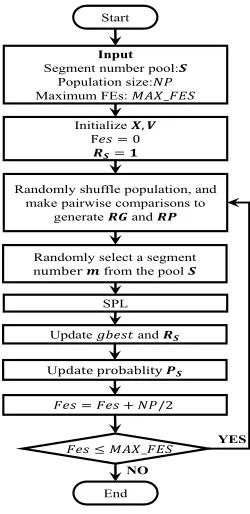
Fig. 3. Framework of DSPLSO.
dynamic segment number, we call as DSPLSO. The perfor-mance of both versions are compared in Section IV-B3 and the comparison results favor DSPLSO.
D. Overall Optimizer and Complexity Analysis
The overall procedure of the proposed DSPLSO is exhib-ited in Fig.3. The execution process of DSPLSO during each generation can be described as follows.
Step 1: First, the whole swarm is randomly organized into pairs and pairwise comparison is executed in each pair to generate the relatively poor particle set RP and the relatively good particle set RG.
Step 2: Then, the roulette wheel selection is conducted to select a segment number from the pool S.
Step 3: Subsequently, SPL is executed for each relatively poor particle in RP as shown in Fig.2.
Step 4: After each generation, gbest is updated and the probabilities Ps of all segment numbers in the pool are recalculated according to (12).
Step 5: If the termination condition is met, the whole pro-cedure exits; otherwise, goes to step 1 to continue.
1) Complexity Analysis: As for the computational
complex-ity, during one generation, from the above steps, we can see that O(NP) is needed to shuffle the swarm and generate RP and RG in step 1, where NP is the swarm size. Step 2 takes constant time and step 3 needs O(NP∗D)to update RP with
O(NP∗D/2)to segment the dimensions of NP/2 particles to be updated and another O(NP∗D/2)to update these particles. To update the probability set Ps in step 4, O(t)is needed with
t being the size of segment number set S, which is a
con-stant and much smaller than NP. To sum up, the complexity of DSPLSO is O(NP∗D+NP+t). Compared with the tradi-tional PSO with complexity O(NP∗D), DSPLSO only needs
O(NP+t)extra in each generation, where the population size
NP and the pool size t are constants far smaller than NP∗D.
Therefore, DSPLSO remains efficient in time complexity.
IV. EXPERIMENTS
To verify the efficiency and effectiveness of DSPLSO, a series of experiments are conducted on CEC’2010 [60] and CEC’2013 [61] large-scale benchmark problems. The CEC’2013 benchmark set (containing 15 functions) is the extension of the CEC’2010 set (consisting of 20 functions). The functions from the CEC’2013 set are more complicated and harder to optimize because of introducing a number of new features, such as imbalance between subcomponents and overlapping functions. The main characteristics of these two function sets are summarized in Tables SI and SII in the sup-plemental material, respectively. For details of these functions, readers can refer to [60] and [61].
In this section, we first empirically investigate the influence of two key parameters in DSPLSO, namely, the popula-tion size NP and the control parameter φ in (7). Then, we will observe the importance of the weighted mean position ˆ
x and the dynamic segment number selection strategy in
SectionsIV-B2andIV-B3, respectively. Subsequently, we will make a wide comparison between DSPLSO and other state-of-the-art algorithms dealing with large-scale optimization in Section IV-C. At last, in Section IV-D, we will observe the scalability of DSPLSO on higher dimensional problems in comparison with CSO [53].
In addition, unless otherwise stated, the maximum number of fitness evaluations is set to 3×10⁶ so that we can make comparisons between DSPLSO and other algorithms which are benchmarked against the same test suite, by citing the results reported in the corresponding papers. Mean value and standard deviation (Std) of results from 30 independent runs are used to evaluate the performance of different algorithms. Besides, in the comparisons between two different algorithms, two-tailed t-tests are performed at a significance level ofα= 0.05, at which the critical t value with 30 samples is 2.064. Additionally, it is worth mentioning that all algorithms are conducted on a PC with 4 Intel Core i5-3470 3.20 GHz CPU, 4 GB memory and Ubuntu 12.04 LTS 64-bit operating system. To save space, some detailed results are not included here but attached to the supplemental material.
A. Parameter Settings
Thus, there remains only one parameter introduced newly in DSPLSO that needs to be fine-tuned, namely φ in (7). A large φ can improve the influence of weighted mean
posi-tion x, possibly leading to a good ability to escape fromˆ
local optima, but this may also lead to slow convergence. Conversely, a small φ may contribute to fast convergence, but it may result in premature convergence easily. So, φ should be tuned. As for the common parameter NP for all EAs, a small swarm size may maintain fast convergence, but cannot afford enough diversity, resulting in premature conver-gence. In contrast, although a large swarm size can increase the diversity of the swarm, it may slow down the conver-gence speed. Thus, a tradeoff between the diversity and the convergence speed should be obtained through selecting a proper NP.
Consequently, to obtain empirical insight into NP and φ, experiments are conducted on DSPLSO with NP varying from 100 to 600 and φ varying from 0 to 0.4 on six CEC’2010 benchmark functions: fully separable and unimodal f1, fully separable and multimodal f3, partially separable and uni-modal f7, and partially separable and multimodal f6, f11, and
f16. Among these functions, more multimodal functions are selected because they are more difficult to optimize than uni-modal functions, resulting in that EAs are more sensitive to parameters on these functions.
Table SIII in the supplemental material exhibits the results with the best ones highlighted for different population sizes along with the corresponding best φ. From this table, we can draw three conclusions.
1) With φ fixed to be a nonzero value, a large NP is preferred. This is because a large NP can afford enough diversity to drag the swarm out of the local areas. However, comparing the results in column “φ = 0.1,” we can see that when NP exceeds 500, the performance of DSPLSO degrades. This may be caused by the slow convergence resulted from the excessive diversity. 2) With NP fixed and larger than 200,φ=0 is preferred,
indicating the importance of the social learning part in (7). However, when φ is larger than 0.1, the perfor-mance of DSPLSO deteriorates dramatically, especially
whenφ >0.2. This is because the social learning part is
over emphasized due to the largerφ, which may result in that particles are dragged far away from the current promising area and the convergence is slowed down. Thus, a largeφ is not preferred.
3) When NP takes a fixed value within [300, 500], the properφ remains unchanged at 0.1.
Based on the above observation, in the following exper-iments related to 1000-D problems, NP = 500 along with
φ = 0.1 is adopted for fair comparison with CSO [53], which shares some similarities with DSPLSO, like evolving all dimensions together, and for which the optimal population size is 500 as well.
B. Observations of DSPLSO
1) Usefulness of the Proposed SPL: In this part, we aim
to verify the usefulness of the developed SPL. Specifically,
we first develop two special cases of the developed SPLSO: 1) SPLSO-1 and 2) SPLSO-1000. The former is the SPLSO with only one segment, which indicates that the whole dimen-sions are considered as a segment and only one predominant particle in RG is selected to guide the learning of particles in RP in (7). The latter is the SPLSO with 1000 segments, which indicates that each dimension is a separate segment for 1000-D problems and SPL would select one predominant par-ticle in RG for the update of each dimension of parpar-ticles in
RP as shown in (7). Then, we can verify the usefulness of
SPL through two comparisons.
1) The comparison between SPLSO-1 and CSO, which can verify the usefulness of SPL under the condition that the whole dimensions of one particle are guided by only one exemplar.
2) The comparison between SPLSO-1000 and CLPSO, which can verify the usefulness of SPL under the con-dition that each dimension of a particle is updated by one exemplar.
Then, we conduct experiments on the twenty 1000-D CEC’2010 functions. To make fair comparisons, the swarm size is set the same (500) for all compared algorithms. Fig. S1 in the supplemental material shows the comparison results.
From this figure, we can see the following.
1) Compared with CSO, SPLSO-1 performs much better on almost all functions, except for five functions, namely
f5, where SPLSO-1 is a little inferior to CSO, and
f13,f15,f18, and f20, where SPLSO-1 and CSO perform very similarly.
2) Compared with CLPSO, SPLSO-1000 are much supe-rior on almost all function as well, except for f10 where SPLSO-1000 is worse than CLPSO.
3) Further, we also can observe that both SPLSO-1 and SPLSO-1000 are much better than CSO and CLPSO on more than 13 functions.
The above experimental results demonstrate that under two extreme conditions, namely considering the whole dimensions as one segment and considering each dimension as a segment, SPLSO is much better than both CSO and CLPSO, verifying the great usefulness of SPL. Compared with the competitive learning strategy in CSO and the comprehensive learning in CLPSO, SPL mainly benefits from the developed PL, where the whole swarm is partitioned into two separate sets RP and
RG and each particle in RG can potentially be the
exem-plar to guide the learning of the particles in RP. These help the swarm in SPLSO maintain high diversity, so that local traps can be avoided, leading to the promising performance of SPLSO.
2) Influence of the Weighted Mean Position: To
substanti-ate the usefulness of weighted mean position x of the swarmˆ
as proposed in (7), first, we use the mean position x to sub-stitute x in (ˆ 7), leading to a version of DSPLSO, denoted as DSPLSO-x. To have a better view on the comparison, the original DSPLSO using x is represented as DSPLSO-ˆ x.ˆ
From this figure, we can see that at the early stage, xˆ
and x have the same effect; but in the late stage, especially when the best solution of the swarm is close to the global or local optima, the solutions obtained by DSPLSO-ˆx are much
better than those obtained by DSPLSO-x, especially on mul-timodal functions as shown in Fig. S2(b), (c), (e), and (f) in the supplemental material. This is mainly because instead of treating all particles equally in x, more emphasis is put on inferior particles in x, which potentially enhances the forceˆ
to drag the swarm to escape from the local areas. Since this weighted mean position operated on the third part in (7) is mainly for promoting the diversity of the swarm, DSPLSO-xˆ
and DSPLSO-x may perform similarly on unimodal func-tions, such as f7 [shown in Fig. S2(d) in the supplemental material], because of the consistence that all particles in the swarm converge to the same direction in the unimodal func-tions. However, DSPLSO-x performs better on multimodalˆ
functions.
Overall, we can see that the weighted mean position x isˆ
promising for DSPLSO in promoting the exploration ability of the swarm, leading to superior performance to x.
3) Influence of the Dynamic Segment Number: To
investi-gate the effectiveness of the dynamic segment number selec-tion strategy in DSPLSO, first, we denote SPLSO with fixed segment number m as “SPLSO-m,” e.g., SPLSO with only one segment can be expressed as “SPLSO-1,” which indicates that the whole dimensions are considered a segment and only one predominant exemplar in RG is selected to guide the learning of each particle in RP. Then we make comparisons between “SPLSO-m” with m ∈ S and DSPLSO on f1, f2, f5, f8, f13, and f18 from the CEC’2010 benchmark set. Fig. S3 in the supplemental material displays the comparison results.
From this figure, it can be found that: 1) on unimodal func-tion f1, SPLSO-1 performs slightly better with respect to the convergence speed, but performs very similarly to other ver-sions of SPLSO, such as DSPLSO and SPLSO with other fixed numbers of segments, in regard to the solution quality. However, when it comes to multimodal functions, like f2, f5,
f8, f13, and f18, SPLSO-1 performs worse than other versions of SPLSO. This is because, for complicated multimodal prob-lems, cooperated with PL, the developed SL can introduce higher diversity owing to letting particles in RP learn from several predominant particles in RG and 2) the optimal num-ber of segments is different for different functions, such as for
f5, the number is 100, while for f13, it is 20. Employing this strategy, DSPLSO can make a good compromise for different functions, which is indicated by that DSPLSO performs very close to or the same as the SPLSO with the optimal segment number. Additionally, the dynamic segment number strategy relieves DSPLSO from the sensitivity to m, liberating users from the tedious effort of fine-tuning m for different problems. Thus, it is beneficial for SPLSO to adopt the dynamic segment number strategy.
C. Comparisons With State-of-the-Art Methods
To better demonstrate the efficiency of DSPLSO, we chose five state-of-the-art and representative algorithms for comparison. Two of them are PSO variants proposed
TABLE I
PARAMETERSETTINGS OF THECOMPARED
ALGORITHMS FOR1000-D PROBLEMS
recently: CSO [53] focusing on the second approach to large-scale optimization as DSPLSO and CCPSO2 [16] con-centrating on the first approach, and the other three are DE variants based on the CC framework [35]: 1) DECC-DG [41]; 2) DECC-G [42]; and 3) MLCC [43], which contribute to the first approach to large-scale optimization with different decomposers.
Furthermore, the parameters in each algorithm are set as recommended in the corresponding papers for fair compar-isons, which is shown in Table I. For MLCC and DECC-G, we directly use the reported results in the Special Session on Large-Scale Global Optimization at CEC’20102 for the CEC’2010 benchmark set, while for the CEC’2013 benchmark set, owing to the missing of reported results of MLCC in the CEC’2013 Special Session, we have to only report the results of DECC-G.3 For CSO, CCPSO2, and DECC-DG, because they were developed in recent two years and have shown their superiority to other methods, we put more emphasis on the comparisons between these three methods and DSPLSO.
TablesIIandIIIpresent the comparison results among dif-ferent algorithms on problems with 1000-D in the CEC’2010 set and the CEC’2013 set, respectively. The highlighted t values mean that DSPLSO is significantly better than the corresponding compared algorithms judged by t values. In addition, in the last two columns of Table II and in the last column of TableIII, we use the highlighted N/As to indicate DSPLSO is much better than MLCC or DECC-G judged by the mean values instead of t values, owing to the absence of the detailed results of MLCC and DECC-G in the corre-sponding special sessions. When using mean values as the comparison standard, if the order of magnitude of mean value of DSPLSO is lower than that of MLCC or DECC-G, we think DSPLSO is significantly better; if the magnitude of mean value of DSPLSO is higher, we think DSPLSO is worse; otherwise, we consider DSPLSO is equivalent to MLCC or DECC-G. Furthermore, we use w/t/l in the last row of both tables to
give the number of wins, ties and losses when DSPLSO com-pares against the counterpart methods. When compared with MLCC and DECC-G, w/t/l are counted by comparing the
mean values of DSPLSO with those of MLCC or DECC-G according to the above mentioned standard.
From these two tables, undoubtedly, we can conclude that DSPLSO outperforms the recent algorithms: CSO (21/35), CCPSO2 (23/35), and DECC-DG (21/35) on most of the func-tions. As for MLCC, DSPLSO displays its superiority on eight functions, and only loses its advantage on two functions on the
2http://nical.ustc.edu.cn/cec10ss.php
TABLE II
COMPARISONRESULTSBETWEENDSPLSOAND THECOMPARED
ALGORITHMS ON20 CEC’2010 BENCHMARKFUNCTIONSWITH
1000-D. THEMEANVALUE ANDSTANDARDDEVIATIONALONG
WITHTWOTAILEDt-TEST ATSIGNIFICANCELEVEL OFα=0.05 WITHRESPECT TOFUNCTIONVALUESAREREPORTEDOVER30
INDEPENDENTRUNS. THEBOLDEDt VALUESMEANTHAT
DSPLSO ISSIGNIFICANTLYBETTERTHAN THE
CORRESPONDINGALGORITHM
CEC’2010 benchmark set. As for DECC-G, DSPLSO domi-nates on 21 functions among all 35 functions. Additionally, we notice that for f1from both CEC’2010 set and CEC’2013 set, though the t-test value between DSPLSO and DECC-DG is smaller than the critical value 2.064, DSPLSO still per-forms significantly better than DECC-DG in terms of mean value and standard deviation. Taking a closer observation, we can see that DSPLSO is better than the CC-based algorithms (CCPSO2, DECC-DG, MLCC, and DECC-G). Compared with CSO, though both algorithms concentrate on the sec-ond approach to large-scale optimization, DSPLSO exhibits its advantages over CSO. The good performance of DSPLSO in comparison with these methods benefits from the pro-posed SPL strategy. On one hand, SPL allows poor particles to learn segments of potentially useful evolution information
TABLE III
COMPARISONRESULTSBETWEENDSPLSOAND THECOMPARED
ALGORITHMS ON15 CEC’2013 BENCHMARKFUNCTIONSWITH
1000-D. THEMEANVALUE ANDSTANDARDDEVIATIONALONG
WITHTWOTAILEDt-TEST ATSIGNIFICANCELEVEL OFα=0.05 WITHRESPECT TOFUNCTIONVALUESAREREPORTEDOVER30
INDEPENDENTRUNS. THEBOLDEDt VALUESMEANTHAT
DSPLSO ISSIGNIFICANTLYBETTERTHAN THE
CORRESPONDINGALGORITHM
from different predominant exemplars, resulting in promising enhancement in both diversity (resulted from learning from different exemplars) and convergence (benefited from learning from predominant exemplars). On the other hand, the random segmentation embedded in SL and performed on each rela-tively poor particle along with the random competition affords potential diversity enhancement. All these together provide strength for DSPLSO to compete with other methods.
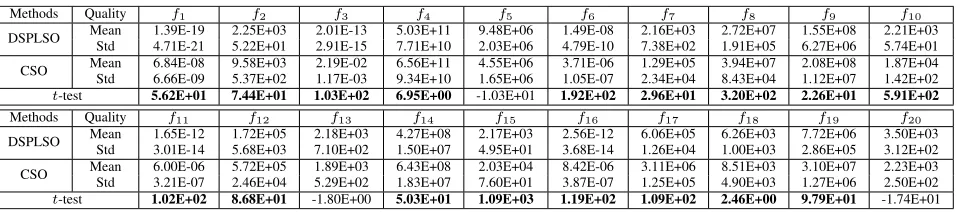
TABLE IV
COMPARISONRESULTSBETWEENDSPLSOANDCSOON20 CEC’2010 BENCHMARKFUNCTIONSWITH2000-D. THEMEANVALUE AND
STANDARDDEVIATIONALONGWITHTWOTAILEDt-TEST ATSIGNIFICANCELEVEL OFα=0.05 WITHRESPECT TOFUNCTIONVALUES
AREREPORTEDOVER30 INDEPENDENTRUNS. THEBOLDEDt VALUESMEANTHATSPLSO ISSIGNIFICANTLYBETTERTHANCSO
From Fig. S4 in the supplemental material, we can see that DSPLSO defeats all the three algorithms on seven func-tions ( f1,f3,f4,f6,f7,f11, and f14) in terms of the quality of solutions and on f13,f18, and f20, though DSPLSO achieves the same best results as CSO, it converges faster. Separately, from the perspective of the quality of solutions, DSPLSO shows its superiority to CCPSO2 [16] on 14 functions, dom-inates CSO [53] on 15 functions, and beats DECC-DG [41] on 12 functions, respectively.
From Fig. S5 in the supplemental material, we can find that DSPLSO defeats all the three methods on three func-tions (f1,f4, and f8) and on f5,f7, and f12, both DSPLSO and CSO achieve the best results. In detail, DSPLSO defeats CSO on six functions, dominates CCPSO2 on nine functions, and beats DECC-DG on ten functions, respectively. Besides, DSPLSO performs similarly to CSO, CCPSO2 and DECC-DG on 5(f3,f5–f7,f12), 1(f11), and 1(f6) functions, respectively.
Comprehensively, on one hand, DSPLSO can find compet-itive or even better solutions than other methods, e.g., shown in Figs. S4(a), (c), and (f) and S5(a) and (d) in the supple-mentary material; on the other hand, DSPLSO can possess a competitive or even faster convergence speed, e.g., shown in Figs. S4(c), (m), (r), and (t) and S5(a) and (l) in the sup-plemental material. All these can be potentially attributed to the proposed SPL, which allows particles to learn from dif-ferent predominant exemplars, enlarging the learning ability of particles. This learning strategy not only brings bene-fits in enhancing diversity for the swarm, leading to good exploration ability, but also potentially promotes the exploita-tion ability, probably resulting in fast convergence and good solutions.
Overall, the experimental results in Tables II and III and the convergence plots in Figs. S4 and S5 in the supplemen-tal material, demonstrate the efficiency and effectiveness of DSPLSO in dealing with large-scale optimization.
D. Scalability to Higher Dimensionality
To further evaluate the scalability of DSPLSO to higher dimensionality, we conduct experiments on DSPLSO for opti-mizing 2000-D problems by modifying the dimension size in the CEC’2010 function generators to 2000.
First, we take a look at the parameter settings of NP and
φ on 2000-D problems with the segment number set S the same as the one used for 1000-D problems. Table SIV in
the supplemental material, presents the experimental results of DSPLSO with NP varying from 200 to 1000 and φ rang-ing from 0.1 to 0.35 on the six functions that are also used for observing the influence of NP andφ on 1000-D problems in Table SIII in the supplemental material, From this table, similar conclusions can be drawn.
1) With NP fixed, a properφis needed. When NP is smaller than 600, φ = 0.1 is preferred; when NP is medium, such as within [600, 800], φ = 0.15 is preferred; and when NP is large, such as 1000, φ=0.2 is preferred. This indicates that when NP becomes large, φ should also choose a properly large value as well.
2) With φ fixed, a large NP is preferred. Comparing the results of DSPLSO with different NP and the corre-sponding bestφ, we can find that a large NP is needed, such as 1000, to afford enough diversity for the opti-mizer to locate the global optima. Above all, we find that NP=1000 andφ=0.2 is the most proper setting for DSPLSO on 2000-D problems.
Then, the comparison between DSPLSO and CSO [53] is conducted. Here, only CSO is selected to make a compari-son because that not only is it the state-of-the-art, but also it belongs to the same approach to large-scale optimization as DSPLSO, which evolves all dimensions together. In addition, NP=1000 andφ=0.15 is adopted for CSO as recommended in [53]. In this series of experiments, the maximum number of fitness evaluations is set to 5×10⁶.
Table IV exhibits the comparison results with highlighted
t values indicating DSPLSO is significantly better than CSO.
From this table, we can see that DSPLSO significantly outper-forms CSO on almost all functions, except for f5 and f20 on which DSPLSO performs worse than CSO and f13 on which DSPLSO and CSO achieve similar performance.
Further, to compare the convergence behaviors of DSPLSO and CSO on 2000-D problems, we conduct experiments on these problems with the number of fitness evaluations varying from 1×10⁶to 1×10⁷. Fig. S6 in the supplemental material shows the comparison results.
The above verified superiority of DSPLSO over CSO mainly benefits from two aspects.
1) Compared with CSO, where the loser is limited to only learn from its corresponding winner, the relatively poor particles in RP in DSPLSO possess better learn-ing ability, due to learnlearn-ing from different predominant exemplars, which is driven by PL.
2) Instead of updating all dimensions using only one exem-plar (the corresponding winner for a loser) in CSO, DSPLSO divides the dimensions of each particle to be updated into several segments, and then evolves the dimensions in each segment together by learning from a randomly selected predominant exemplar, which is driven by SL. For different dimension segments, the exemplars may be different. This learning strategy has the potential to gather the useful information in differ-ent exemplars together. The cooperation between SL and PL leads to SPL, which can afford promising exploration and exploitation abilities.
All in all, this series of experiments demonstrate the good scalability of DSPLSO to higher dimensionality.
V. CONCLUSION
This paper has proposed a novel SPLSO. To self-adaptively determine the appropriate number of segments for dif-ferent problems, borrowing ideas from MLCC [43] and CCPSO2 [16], we designed a segment number pool to dynam-ically select a proper segment number, leading to DSPLSO. This new optimizer allows the relatively poor particles to learn from different good particles through the SPL. The SPL strategy may contribute to fast convergence and high diver-sity to some extent, which are verified by the experiments on two widely used large-scale problem sets—the CEC’2010 and CEC’2013 benchmark function sets. The comparison results between DSPLSO and different state-of-the-art algorithms demonstrate the competitive feasibility and efficiency of the new optimizer. Additionally, the experimental results on 2000-D problems further substantiate the competitive scalability of DSPLSO to higher dimensionality.
Though DSPLSO has shown its ability in dealing with large-scale optimization, at times it still falls into local optima. For instance, the results on f5,f8,f9, and f14 shown in TableIIand on f4,f8,f11, and f13 shown in TableIIIare far away from the global optima. This is unfortunately a common drawback for other optimization algorithms as well. Our future research is to investigate how to mitigate the trapping at local optima and further enhance the performance of DSPLSO.
REFERENCES
[1] M. Dorigo, M. Birattari, and T. Stutzle, “Ant colony optimization,” IEEE
Comput. Intell. Mag., vol. 1, no. 4, pp. 28–39, Nov. 2006.
[2] K. V. Price, R. M. Storn, and J. A. Lampinen, Differential Evolution:
A Practical Approach to Global Optimization. New York, NY, USA:
Springer, 2006.
[3] M. Clerc, Particle Swarm Optimization, vol. 93. Hoboken, NJ, USA: Wiley, 2010.
[4] R. A. Sarker, M. Mohammadian, and X. Yao, Evolutionary Optimization, vol. 48. New York, NY, USA: Springer, 2002.
[5] I. Fister, Jr., M. Perc, S. M. Kamal, and I. Fister, “A review of chaos-based firefly algorithms: Perspectives and research challenges,” Appl.
Math. Comput., vol. 252, pp. 155–165, Feb. 2015.
[6] Y. Zhang, Y.-J. Gong, H. Zhang, T.-L. Gu, and J. Zhang, “Towards fast niching evolutionary algorithms: A locality sensitive hashing-based approach,” IEEE Trans. Evol. Comput., in press, 2016.
[7] P. Faria, J. Soares, Z. Vale, H. Morais, and T. Sousa, “Modified par-ticle swarm optimization applied to integrated demand response and DG resources scheduling,” IEEE Trans. Smart Grid, vol. 4, no. 1, pp. 606–616, Mar. 2013.
[8] M. Shen et al., “Bi-velocity discrete particle swarm optimization and its application to multicast routing problem in communication networks,”
IEEE Trans. Ind. Electron., vol. 61, no. 12, pp. 7141–7151, Dec. 2014.
[9] J. Zhang, C. Zhang, T. Chu, and M. Perc, “Resolution of the stochas-tic strategy spatial prisoner’s dilemma by means of parstochas-ticle swarm optimization,” PloS One, vol. 6, no. 7, 2011, Art. no. e21787. [10] I. Fister et al., “Particle swarm optimization for automatic creation
of complex graphic characters,” Chaos Solitons Fractals, vol. 73, pp. 29–35, Apr. 2015.
[11] X. Wen et al., “A maximal clique based multiobjective evolutionary algo-rithm for overlapping community detection,” IEEE Trans. Evol. Comput., in press, 2016.
[12] X.-Y. Zhang et al., “Kuhn–Munkres parallel genetic algorithm for the set cover problem and its application to large-scale wireless sensor networks,” IEEE Trans. Evol. Comput., vol. 20, no. 5, pp. 695–710, Oct. 2016.
[13] Z.-H. Zhan, J. Zhang, Y. Li, and H. S.-H. Chung, “Adaptive particle swarm optimization,” IEEE Trans. Syst., Man, Cybern. B, Cybern., vol. 39, no. 6, pp. 1362–1381, Dec. 2009.
[14] M. Campos, R. A. Krohling, and I. Enriquez, “Bare bones particle swarm optimization with scale matrix adaptation,” IEEE Trans. Cybern., vol. 44, no. 9, pp. 1567–1578, Sep. 2014.
[15] J. Kennedy, “Bare bones particle swarms,” in Proc. IEEE Swarm Intell.
Symp., Indianapolis, IN, USA, 2003, pp. 80–87.
[16] X. Li and X. Yao, “Cooperatively coevolving particle swarms for large scale optimization,” IEEE Trans. Evol. Comput., vol. 16, no. 2, pp. 210–224, Apr. 2012.
[17] R. Eberhart and J. Kennedy, “A new optimizer using particle swarm theory,” in Proc. 6th Int. Symp. Micro Mach. Human Sci., vol. 1. Nagoya, Japan, 1995, pp. 39–43.
[18] J. Kennedy and R. Eberhart, “Particle swarm optimization,” in Proc.
IEEE Int. Conf. Neural Netw., vol. 4. Piscataway, NJ, USA, 1995,
pp. 1942–1948.
[19] Y.-J. Gong et al., “Genetic learning particle swarm optimization,” IEEE
Trans. Cybern., vol. 46, no. 10, pp. 2277–2290, Oct. 2016.
[20] W.-N. Chen et al., “A novel set-based particle swarm optimization method for discrete optimization problems,” IEEE Trans. Evol. Comput., vol. 14, no. 2, pp. 278–300, Apr. 2010.
[21] W.-N. Chen et al., “Particle swarm optimization with an aging leader and challengers,” IEEE Trans. Evol. Comput., vol. 17, no. 2, pp. 241–258, Apr. 2013.
[22] Q. Fan and X. Yan, “Self-adaptive differential evolution algorithm with zoning evolution of control parameters and adaptive mutation strategies,”
IEEE Trans. Cybern., vol. 46, no. 1, pp. 219–232, Jan. 2016.
[23] X. Qiu, K. C. Tan, and J.-X. Xu, “Multiple exponential recombination for differential evolution,” IEEE Trans. Cybern., in press, 2016. [24] Q. Yang et al., “Adaptive multimodal continuous ant colony
optimiza-tion,” IEEE Trans. Evol. Comput., in press, 2016.
[25] T. Liao, K. Socha, M. A. M. de Oca, T. Stützle, and M. Dorigo, “Ant colony optimization for mixed-variable optimization problems,” IEEE
Trans. Evol. Comput., vol. 18, no. 4, pp. 503–518, Aug. 2014.
[26] P. Yang, K. Tang, and X. Lu, “Improving estimation of distribution algorithm on multimodal problems by detecting promising areas,” IEEE
Trans. Cybern., vol. 45, no. 8, pp. 1438–1449, Aug. 2015.
[27] Q. Yang et al., “Multimodal estimation of distribution algorithms,” IEEE
Trans. Cybern., in press, 2016.
[28] I. Fister, I. Fister, Jr., X.-S. Yang, and J. Brest, “A comprehensive review of firefly algorithms,” Swarm Evol. Comput., vol. 13, pp. 34–46, Dec. 2013.
[29] J. Kennedy, “Stereotyping: Improving particle swarm performance with cluster analysis,” in Proc. IEEE Congr. Evol. Comput., vol. 2. La Jolla, CA, USA, 2000, pp. 1507–1512.
[30] Z. Ren, A. Zhang, C. Wen, and Z. Feng, “A scatter learning particle swarm optimization algorithm for multimodal problems,” IEEE Trans.