Applications in Wireless
Communications
Ni Ding
A thesis submitted for the degree of
Doctor of Philosophy
The Australian National University
I would like to give my sincere thanks to my supervisors, Professor Rodney A. Kennedy and Professor Parastoo Sadeghi, for their guidance, support and encour-agement throughout my PhD studies. They have given me freedom and flexibility in pursuing my research interests and explore new ideas, which have found their way into this thesis. I would also like to acknowledge the support from the College of Engineering and Computer Science for assisting with the transfer of my PhD from Sydney to Canberra and for providing the excellent research environment and facili-ties. I also acknowledge the helpful discussions with the friendly people in the signal processing and communications groups in the Research School of Engineering, the Australian National University.
I would like to thank Professor Chung Chan for the great time discussing and understanding in depth the potential of my research works when I was visiting the Chinese University of Hong Kong from Nov 1, 2015 to Feb 9, 2016. I would like to thank Professor Tie Liu for the warm welcome and nice discussions when I was visiting the Texas A&M University from Feb 13, 2016 to Mar 12, 2016.
In addition to those supports to my research works, I would like to thank my friend, Wei (Wendy) Dong, Guofeng (Eric) Zhang, little Edward Zhang and Manli Xu for helping me settle down in Canberra and all the nice time and great fun that we had when we were sightseeing the places inside and around Canberra and analyzing and practicing the cooking recipes.
This monograph studies the submodularity in wireless communications and how to use it to enhance or improve the design of the optimization algorithms. The work is done in three different systems.
In a cross-layer adaptive modulation problem, we prove the submodularity of the dynamic programming (DP), which contributes to the monotonicity of the optimal transmission policy. The monotonicity is utilized in a policy iteration algorithm to relieve the curse of dimensionality of DP. In addition, we show that the monotonic optimal policy can be determined by a multivariate minimization problem, which can be solved by a discrete simultaneous perturbation stochastic approximation (DSPSA) algorithm. We show that the DSPSA is able to converge to the optimal policy in real time.
For the adaptive modulation problem in a network-coded two-way relay channel, a two-player game model is proposed. We prove the supermodularity of this game, which ensures the existence of pure strategy Nash equilibria (PSNEs). We apply the Cournot tatonnement and show that it converges to the extremal, the largest and smallest, PSNEs within a finite number of iterations. We derive the sufficient conditions for the extremal PSNEs to be symmetric and monotonic in the channel signal-to-noise (SNR) ratio.
Acknowledgments vii
Abstract ix
1 Introduction 1
1.1 Submodularity on vector lattice . . . 1
1.1.1 Monotonic Optimal Decision . . . 1
1.1.2 Strategic Complementarities . . . 4
1.2 Submodularity on set lattice . . . 5
1.3 Contributions . . . 6
1.3.1 Cross-layer Adaptive Modulation . . . 7
1.3.2 Adaptive Modulation in Two Way Relay Channel . . . 9
1.3.3 Communication for Omniscience . . . 10
1.4 Thesis Outline . . . 12
2 Preliminaries 15 2.1 Partially Ordered Set . . . 15
2.2 Lattice . . . 16
2.3 Submodularity . . . 17
2.3.1 Parametric Submodular Function . . . 17
2.3.1.1 Monotone Comparative Statics . . . 18
2.3.1.2 Tarski Fixed Point Theorem . . . 19
2.3.2 Submodular Set Function . . . 20
2.3.2.1 Submodular Function Minimization . . . 21
2.3.2.2 Dilworth Truncation . . . 22
2.4 Notations . . . 22
3 Cross-layer Adaptive Modulation 23 3.1 System . . . 25
3.3 Objective . . . 28
3.4 Dynamic Programming . . . 29
3.5 Monotonic Optimal Transmission Policy . . . 30
3.5.1 Nondecreasing Optimal Policy in Queue State . . . 31
3.5.2 Nondecreasing Optimal Policy in Queue and Channel States . . 32
3.5.3 Examples . . . 34
3.6 Monotonic Policy Iteration . . . 36
3.7 Discrete Simultaneous Perturbation Stochastic Approximation . . . 39
3.7.1 Obtaining Gradients . . . 41
3.7.2 Simulated Objective Function . . . 42
3.7.3 Step Size Parameters and Penalty Coefficient . . . 43
3.7.4 Complexity and Convergence Performance . . . 43
3.8 Summary . . . 47
Appendices . . . 50
3.A Monotonicity ofQinbin Proof of Theorem 3.5.5 . . . 50
3.B L\-convexity of Qin(b,a)in Proof of Theorem 3.5.5 . . . 50
3.C L\-convexity of ˆV(y,f,h)inyin Appendix 3.B . . . 51
3.D First Order Stochastic Dominance . . . 51
3.E Proof of Submodularity ofQin(b,h,a)in Theorem 3.5.7 . . . 52
4 Adaptive Modulation in Two-way Relay Channel 53 4.1 System . . . 56
4.2 Game Formulation . . . 57
4.2.1 Two-player Game model . . . 58
4.2.2 Nash Equilibria . . . 59
4.2.3 Single-agent Adaptive Modulation . . . 60
4.3 Pure Strategy Nash Equilibrium . . . 60
4.3.1 Existence and Cournot Tatonnement . . . 62
4.3.2 Simulation Results . . . 63
4.3.3 Pareto Order of Extremal PSNEs . . . 67
4.4 Symmetry and Monotonicity of Nash Equilibria . . . 67
4.5 Summary . . . 73
Appendices . . . 74
4.B Proof of Theorem 4.4.1 . . . 74
4.C Proof of Corollary 4.4.4 . . . 75
5 Communication for Omniscience 77 5.1 Introduction . . . 77
5.2 System Model . . . 81
5.2.1 Asymptotic and Non-asymptotic Models . . . 82
5.2.2 Finite Linear Source Model and CCDE . . . 82
5.3 Minimum sum-rate and Optimal Rate Vector . . . 85
5.3.1 Preliminaries . . . 86
5.3.2 Nonemptiness of the Base Polyhedron . . . 86
5.3.3 Minimum Sum-rate . . . 89
5.3.4 Related Results . . . 93
5.3.5 Secrecy Capacity and Multivariate Mutual Information . . . 96
5.4 Lower Bound on Minimum Sum-Rate . . . 96
5.5 Algorithms for the Minimum Sum-rate CO Problem . . . 98
5.5.1 Principal Sequence of Partitions (PSP) . . . 100
5.5.2 Modified Decomposition Algorithm . . . 103
5.5.3 Coordinate-wise Saturation Capacity Algorithm by Fusion Method105 5.5.3.1 Coordinate-wise Saturation Capacity (CoordSatCap) Algorithm . . . 106
5.5.3.2 A Fusion Method Implementation . . . 110
5.5.4 Solutions for the Finite Linear Source Model . . . 113
5.5.5 Complexity . . . 116
5.5.5.1 CoordSatCapFus vs. CoordSatCap . . . 117
5.5.5.2 MDA algorithm . . . 117
5.5.5.3 SIA algorithm . . . 119
5.6 Minimum Weighted Sum-rate Problem . . . 121
5.7 Fundamental Partition: Minimal Separators . . . 122
5.7.1 Properties of Minimal/Finest Separators . . . 123
5.7.2 Separable Convex Function Minimization . . . 125
5.8 Complimentary User Subset for Successive Omniscience . . . 127
5.9 Summary . . . 134
5.A Lemma 5.A.1 in Proof of Theorem 5.3.3 . . . 136
5.B Proof of Theorem 5.5.5 . . . 136
5.C Tight Sets and CoordSatCap Algorithm . . . 137
5.C.1 Edmond Greedy Algorithm . . . 139
5.D Proof of Lemma 5.5.10 . . . 139
5.E Proof of Lemma 5.5.11 . . . 140
5.F Fundamental PartitionP∗ noncrossing ˆX φi . . . 140
5.G Submodular Function Minimization Algorithms . . . 141
5.H Divide-and-conquer Algorithm . . . 142
5.I Proof of Theorem 5.7.2 . . . 144
5.J Integral Rate Increment Method for Fairness . . . 145
5.K Proof of Theorem 5.8.5 . . . 145
5.L Proof of Theorem 5.8.8 . . . 146
6 Conclusion 147 6.1 Future Work . . . 147
Introduction
Submodularity refers to the property of functions defined on lattice [1–3].1 While it has been known in economics for a long time, submodularity also naturally appears in many other fields, e.g., operations research, computer science and graph theory. It is shown that the submodularity imposes a structure which allows much stronger mathematical results than we would be able to achieve without it [4]. These struc-tured results have been widely used in various optimization problems recently and these applications are based on two main groups: submodularity on vector lattice and submodularity on set lattice.
1
.
1
Submodularity on vector lattice
In economics, the comparative statics compares one static condition, equilibrium or economic outcome with another [5, 6]. It is used to study how the equilibrium state varies after a change in some underlying exogenous parameter. A typical application is in the study of markets [7]: Comparative statics is used to analyze how the equi-librium price and quantity are affected by the variations in the demand and supply determinants. It has also been used in the studies on monetary and fiscal policies in [8, 9].
1.1.1 Monotonic Optimal Decision
In [1], Topkis studied the monotone comparative statics based on the submodularity on the vector lattice. It is shown that, for a parametric submodular cost function
that is defined on a vector lattice, the best response of a decision maker is monoton-ically nondecreasing in the exogenous parameter. When the exogenous parameter describes the condition of the environment, e.g., market price, temperature and stor-age, the best decision rule, or the optimal policy, is a nondecreasing function in the environment/system state. This result has been widely used to study various economic problems or behaviors. For example, in [10], it is proved that the submod-ularity of the cost function is the necessary and sufficient condition for the variation of the welfare to be monotonically nondecreasing in income, which also relieves the smoothness assumption so that the result applies to the case when the domain of the cost function is discrete; in [11], a study on the stopping problem shows that the submodularity ensures that the optimal project stopping time that maximizes a discounted cash flow is nonincreasing in the discount factor.
Although statics refers to the equilibrium status rather than an evolutional pro-cess, the study of monotone comparative statics can be easily extended to dynamic or stochastic models. In [12], the author studied the submodularity, log-submodularity and single-crossing properties of the expected cost functions to show the monotone comparative statics in the stochastic decision making problems. While these results have been applied to various problems such as the optimal portfolio investment in [13,14], the main applications appear predominantly in the inventory and produc-tion models in operaproduc-tions research. Based on Markov decision process (MDP) model, it is shown in [15, 16] that the optimal control of an inventory system with one prod-uct and two categories of customers is fully characterized by a switching curve due to the submodularity of the dynamic programming (DP). In [17, 18], the monotonic-ity of optimal appointment management in the primary-care clinics is also proved based on the submodularity. It turns out that the transmission control problem in many wireless communications systems, e.g., the buffer departure management in data link layer, can be also fully characterized by the monotone comparative statics in the queue occupancy control in [19–22].
of the wireless channel so as to improve the average transmission error rate. Since the data generating process and the variation of the channel signal-to-noise (SNR) ratio are stochastic,2there is a cross-layer transmission control problem that is formulated in [23–27]: how to make sequential decisions on determining the transmission rate in each symbol durations so that the long-term costs incurred by the queueing effects in the data link layer and transmit error rate and/or spectral efficiency in the physical layer are minimized. The authors in [24–26] derived the stationary probability of the queue occupancy to estimate the long-term average cost so that the optimal policy could be searched by linear programming (LP). Whereas the authors in [28–33] con-sidered discounted infinite horizon MDP model so that the optimal solution could be found by dynamic programming (DP): policy or value iteration [34]. For the latter case, the monotonicity of the optimal randomized policy in queue occupancy/state is proved or established in [30–33] based on the submodularity of DP.
However, in the majority of the existing studies on monotone comparative statics in cross-layer transmission control problems, the existence of the submodularity is only proved under certain conditions. For example, in [28], the submodularity of the state transition probability is proved by assuming uniformly distributed traffic rates. In [30], the strict submodularity of DP is assumed to be preserved by a weight factor in the cost function, where, however, the exact value of this factor is not given. On the other hand, most of these studies only prove the monotonicity of the optimal transmission policy in the queue state.3 It remains unclear if there exists an optimal
deterministic policy that is monotonically varying in both queue and channel states. And, if so, it is worth discussing whether the monotonicity exists naturally or with less constraints imposed on the message arrival statistics or the parameters in the cost function.
In addition, there is also a problem of how to utilize the monotonicity to facilitate the optimal policy learning process. There are some developments in the existing literature. For example, based on the monotonicity of the optimal policy, the authors in [32] adapted the DP to a monotonic policy iteration (MPI) algorithm and the au-thors in [28, 31] proposed a stochastic approximation algorithm. It has been shown that both approaches are able to relieve the curse of dimensionality4 of DP for deter-2Stochastic data generating process means that the quantity of messages generated by mobile devices is random.
3These works can be summarized by the monotone comparative statics on queue departure control in [21].
brute-mining a monotonic randomized optimal policy. While the studies in [28, 31, 32] are based on a constrained MDP model, it remains of interest if the submodularity exists in a cross-layer transmission control problem that is modeled by an unconstrained MDP model and, if so, whether the submodularity contributes to the existence of a deterministic, rather than randomized, optimal transmission policy. Most important of all, we are interested in whether the MPI and stochastic approximation algorithms can be still applied for determining this monotonic deterministic optimal policy and whether the convergence performance and/or complexity can be improved or not.
1.1.2 Strategic Complementarities
On the other hand, in a multi-agent decision-making problem, when the exogenous parameter in the monotone comparative statics refers to the strategies taken by other decision makers, the strategies of all decision makers reinforce each other. This sce-nario is called strategic complementarities [36]. In [37], Tarski proved that the fixed points of a nondecreasing function or mapping from a nonempty complete lattice to itself formed a nonempty complete lattice. Consequently, in [38], Davis relaxed the complete lattice constraint to lattice, i.e., it was proved that the fixed points of a nondecreasing mapping from a lattice to itself formed a complete lattice which was necessarily nonempty. In a non-cooperative game with strategic complementarities, i.e., when the cost functions of all players in the game are submodular, these results ensure the existence of not only the Nash equilibrium in pure strategy form, but also the extremal equilibria, the largest and smallest equilibria [39, 40].
In economics, the concept of supermodular game5 has been used to relieve the
constraints for the existence of the structured results in industrial organization anal-ysis. For example, in [41], the existence of multiple equilibria in the Cournot market was proved based on the strategic complementarities, which does not require the quasi-convexity of the cost functions; in [42], the taxonomy of strategic behavior was proved just based on the monotonicity of the marginal payoffs, which relaxes the assumption of the existence of a unique and stable market equilibrium in the second stage of the game.
In wireless communications, there is a problem of how to control the transmitters’
force search way [34], due to which the complexity grows large in the cardinality of the state space of MDP. This problem is called thecurse of dimensionality[35].
powers so as to minimize the interference and this problem is usually modeled by a supermodular game [43]. In [44], the authors introduced a price mechanism to the wireless power management problem, where the pricing function is a linear function of the transmit power and its supermodularity is used to improve the Nash equilib-rium by Pareto domination. In [45–47], the distributed power control problem was considered and the existence, uniqueness and stability of the Nash equilibrium were studied. In [48], the power control problem was formulated as a repeated supermod-ular game, where the authors proposed a reinforcement learning algorithm based on stochastic fictitious play and proved its convergence to the Nash equilibrium.
While the supermodular game model is frequently seen as an analysis tool in the power control problems, it remains of interest if the strategic complementarities ap-pears in other multi-agent optimization problems in wireless communications. And, if so, does the supermodularity of the game ensure the existence of the equilibria and how is the performance of these equilibria in terms of the quality of wireless transmissions, e.g., BER, interference and spectral efficiency. On the other hand, the existing literature in wireless communications does not shed light on the difference between the largest and smallest equilibria. The Pareto order of the equilibria in the supermodular game is revealed in [39, 40]. Therefore, it would be of interest to see if this Pareto order results in some preference or priority order of the equilibria in the practical applications in wireless communications.
1
.
2
Submodularity on set lattice
In [49], Fujishige studied the combinatorial optimization problem based on submod-ularity on set lattice, where it is proved that a submodular set function can be min-imized in strongly polynomial time. There are many examples of submodular set functions, e.g., the cut function of a graph [50], the rank function of a matroid [51] and the weighted coverage function [52].
optimiza-tion problems which can be directly used to fully characterize the cut-set bounds of the broadcast channels. In [55], the wireless relay network in [56] is studied based on a flow model called linking system and the max-flow min-cut theorem and sub-modularity of the cut function are proved, based on which an efficient algorithm is proposed to determine the maximum flow. It is shown that this algorithm can be easily adapted to determine the minimum costs that are incurred at the inputs and outputs of the relays.
On the other hand, the emerging studies on the information-theoretic network coding problems continue to use the submodularity of the entropy function. In [57], it is shown that every entropy function is the rank of a polymatroid, a subset of the submodular set functions. In [58], it is shown that the channel capacity upper bound in a multiaccess fading channel is a polymatroid rank function. In network coding, while some problems of the optimal recovery of messages, e.g. [54], can be described by a graph model which depicts the information flow in the network, many of them still directly deal with the entropy function, e.g., [59–61], for which the max-flow min-cut algorithms such as [62–64] do not apply. In these cases, it is worth discussing whether the combinatorial optimization problem under consideration can be reduced to SFM problems, due to the submodularity of the entropy function, so that it can be solved in polynomial time.
1
.
3
Contributions
In this monograph, we look into three different optimization problems in wireless communications. We study the optimization problems in these systems and prove the existence of the submodularity on both vector and set lattices. We show how to utilize the submodularity to propose efficient algorithms for solving the optimiza-tion problems under consideraoptimiza-tion. We also introduce new concepts, e.g., the L\ -convexity and principal sequence of partitions (PSP). We show that these properties can be used to refine and/or improve the results on monotone comparative statics and combinatorial optimizations in wireless communications.
packets
scheduler
FIFO queue
m-QAM
transmitter wireless fading channel
[image:21.595.119.514.111.214.2]data link layer physical layer
Figure 1.1: Cross-layer adaptive m-QAM system. The packet arrival process is stochastic. The number of bits in the QAM symbol is controlled by the scheduler.
studies on a queue-assisted cross-layer adaptive modulation problem, an adaptive modulation problem in the network-coded two-way relay channel (NC-TWRC) and the problem of communication for omniscience (CO).
1.3.1 Cross-layer Adaptive Modulation
We study the monotone comparative statics in the optimal transmission policy of a cross-layer adaptive m-quadrature amplitude modulation (m-QAM) problem in Fig. 1.1. In this system, it is assumed that the packets originated from data-generating devices are buffered by a finite-length first-in-first-out (FIFO) queue in the data link layer. The packets that leave the queue are transmitted over a wireless channel in the physical layer by m-QAM modulation. The number of packets departing the queue, or the constellation sizemin them-QAM modulation, is controlled by a scheduler.
We model this cross-layer adaptive modulation system by an MDP and derive sufficient conditions for the existence of a monotonic optimal transmission policy in both queue and channel states based on the submodularity and L\-convexity of
DP. We also utilize the monotonicity to propose two low complexity algorithms, monotonic policy iteration (MPI) based on L\-convexity and discrete simultaneous
perturbation stochastic approximation (DSPSA), to relieve the curse of dimension of DP.
Our main contributions in the cross-layer adaptive m-QAM problem are as fol-lows.
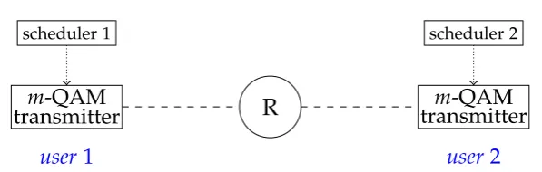
scheduler 1
m-QAM
transmitter
R
scheduler 2
m-QAM transmitter
[image:22.595.126.425.103.198.2]user1 user2
Figure 1.2: Adaptivem-QAM modulation in network-coded two-way relay channel. The relay is denoted by node ’R’.
of the optimal policy in the queue state: The increment of the optimal pol-icy between adjacent queue states is no greater than one, i.e., if the optimal modulation scheme is 2a-QAM for a certain queue state, then the optimal mod-ulation scheme for its adjacent queue states must be 2a-QAM, 2(a+1)-QAM or 2(a−1)-QAM.
• By observing the submodularity of DP, we derive the sufficient conditions for the optimal policy to be nondecreasing in both queue and channel states. We show that these conditions are satisfied if the channel experiences slow and flat fading and a proper value of the weight factor, a coefficient in the immediate cost function in MDP, is chosen.
• We utilize the bounded marginal effect to propose an MPI algorithm for search-ing the monotonic optimal policy based on the L\-convexity of DP. It is shown that the time complexity of MPI based onL\-convexity is much lower than the one based on submodularity that is proposed in [32, 33] and DP.
1.3.2 Adaptive Modulation in Two Way Relay Channel
For the network-coded two-way relay channel (NC-TWRC) in Fig. 1.2, we assume that adaptivem-QAM modulation is implemented at each of the two end users. The superposition of them-QAM symbols from the users are broadcast by a relay which adopts an amplify-and-forward physical layer network coding scheme. Let the adap-tive modulation be done in the physical layer only, instead of cross-layer. We reveal the strategic complementarities in this adaptive modulation problem and propose a two-player supermodular game model, where pure strategy Nash equilibria (PSNEs) always exist. We show the performance of the extremal, the largest and smallest, PSNEs in terms of BER and spectral efficiency and derive sufficient conditions for the symmetry and monotonicity of them in the SNRs of two user-to-user channels.
Our main contributions in the adaptivem-QAM problem in the NC-TWRC are as follows.
• We propose a two-player game model that is parameterized by the SNRs of two user-to-user channels. The purpose is to determine the joint strategies of users, the bit rates of bothm-QAM transmitters, such that the transmission error rate and spectral efficiency in the NC-TWRC are optimized.
• We prove the supermodularity of this two-player game which ensures the ex-istence of PSNEs due to Tarski fixed point theorem. We show that the largest and smallest PSNEs can be searched by Cournot tatonnement [66] which con-verges in a finite number of iterations. We run simulations to show that the extremal PSNEs are superior to the conventional single-agent adaptive modu-lation schemes in enhancing the spectral efficiency in the NC-TWRC system.
• We reveal the Pareto order of extremal PSNEs: The smallest PSNE Pareto dom-inates the largest one. Therefore, the smallest PSNE is always preferred to the largest one by both users.
user 1
z1={Wa,Wb,Wc,Wd,We}
user 2
z2 ={Wa,Wb,Wf} user 3
z3={Wc,Wd,Wf}
Figure 1.3: Coded cooperative data exchange (CCDE) system, an example of the communication for omniscience (CO) problem. Each Wj denotes a packet. User i
obtains zi, a subset of the packet set {Wa, . . . ,Wf}. The users want to obtain the
whole packet set by transmitting linear combinations of zis via lossless broadcast channels.
1.3.3 Communication for Omniscience
Finally, we consider the communication for omniscience (CO) problem: A set of users observe a discrete memoryless multiple source and want to recover the entire multiple source via communications. The 3-user coded cooperative data exchange (CCDE) in Fig. 1.3 is an example of the CO problem. It is assumed that each user obtains a portion of a packet set. The users transmit linear combinations of packets via error-free broadcast channels in order to help each other recover the packet set. We study the problem of how to attain omniscience with the minimum sum-rate, the total number of communications, and determine a corresponding optimal rate vector. The results cover both asymptotic and non-asymptotic models where the transmission rates are real and integral, respectively.
over a merged user set. We show by experiment results that this fusion method contributes to a reduction in computation complexity as compared to the original CoordSatCap algorithm.
Our main contributions in the CO problem are as follows.
• Based on the SW constraints, we define an intersecting submodular function that is parameterized by the value of the sum-rate. We show that the existence of an omniscience-achievable rate vector with the designated sum-rate is equiv-alent to the nonemptiness of the base polyhedron of this function, which can be determined by a necessary and sufficient condition on the Dilworth trunca-tion. Based on this condition, the minimum sum-rate in both asymptotic and non-asymptotic models can be determined via a maximization problem, which determines the highest lower bound on the achievability of the sum-rate im-posed by the SW constraint over all multi-way cuts of the user set. The finest maximizer of this problem is called the fundamental partition and denoted by
P∗.
• The optimal rate vector set, the set that contains all the omniscience-achievable rate vectors with the minimum sum-rate, is described by a submodular base polyhedron. The extreme points, or vertex, in this submodular base polyhedron are the fractional and integral optimal rate vectors in the asymptotic and non-asymptotic models, respectively.
mini-mum sum-rate in the non-asymptotic model. It is also shown that by choosing a proper linear ordering of the user indices, the optimal rate vectors returned by the MDA and SIA algorithms also minimize a weighted sum-rate function in the optimal rate vector set.
• We show that both MDA and SIA algorithms can be broken down into the tasks of solving SFM problems so that both algorithms complete in polynomial time. We compare the experiment results between the CoordSatCap and Co-ordSatCapFus algorithms. It is shown that the fusion method contributes to a reduction in computation complexity as compared to the CoorSatCap algo-rithm that is implemented in [67, 68] and the reduction is considerable when the number of users grows.
• We show that the fundamental partition P∗ is the minimal separator of a sub-modular function which gives rise to the decomposition property of P∗ in the asymptotic model: The separable convex function minimization problem over the optimal rate vector set can be broken into|P∗|subproblems, each of which formulates the separable convex function minimization problem that is defined on one element or user subset in P∗. These subproblems can be solved sepa-rately so that the overall complexity is reduced. The minimizer of this separable convex function minimization problem usually gives a fair rate allocation in the optimal rate vector set in the asymptotic model.
• We show that a complimentary user subset can be searched by the SFM algo-rithms, which allows the omniscience to be achieved in a successive manner: The local omniscience can be attained first without increasing the minimum sum-rate for attaining the global omniscience eventually.
1
.
4
Thesis Outline
In Chapter 3, we look into a cross-layer adaptive m-QAM modulation problem, where we show that the submodularity of the dynamic programming (DP) con-tributes to the monotonicity of the optimal transmission policy based on which we discuss how to relieve the complexity of DP. This chapter contributes to the author’s work in [69].
In Chapter 4, we model the adaptive m-QAM modulation problem in the NC-TWRC by a two-player game and prove the existence, symmetry and monotonicity of PSNEs. This chapter contributes to the author’s work in [70].
In Chapter 5, we study the CO problem based on the submodularity of the en-tropy function. We propose polynomial time algorithms for determining the mini-mum sum-rate and a corresponding optimal rate vector, discuss some properties of the fundamental partition and show how to achieve the omniscience in a successive manner. This chapter contribute to the author’s works in [71–76].
Preliminaries
Submodularity is a property that is defined on the lattice, where the lattice could be a set of vectors or a set space. In this thesis, the studies in Chapters 3 and 4 are based on the submodularity on a vector lattice, while the studies in Chapter 5 are based on the submodularity on a set lattice. In this chapter, we introduce the concepts of partially ordered sets and lattices, briefly show the submodularity in different types of lattices and describe how they are applied to the works in this thesis. The contents in Sections 2.1 and 2.2 are based on the studies in [1, 49].
2
.
1
Partially Ordered Set
For a setL,is abinary relationif, for alla,b∈ L, eithera bor a6b. In addition, if abanda 6=b, we denotea≺ b. If the binary relationship is
• reflexive: for all a∈ L,a a;
• antisymmetric: for alla,b∈ L, ifabandab, thena= b;
• transitive: for alla,b,c∈ L, if abandbc, thena c,
Lis called apartially ordered set (poset)with respect to and we denote this poset by
(L,). In the poset(L,), ifabfor two elements a,b∈ L, we say thataandbare ordered; ifa 6b, aand bare unordered. A poset is achainif it does not contain any unordered pair of elements.
Example 2.1.1. LetRK be an K-dimension real number space. ≤ is the binary relation
de-fined on RK such that, for x,x0 ∈ RK, x ≤ x0 if x
i ≤ x0i for all i ∈ {1, . . . ,K}. Then,
(RK,≤) is a poset. Let Ri = [li,ui] ⊆ R for all i ∈ {1, . . . ,K}. For R = ×Ki=1Ri,
posets, e.g., (ZK,≤) and (Z,≤), where Z = ×K
i=1Zi with Zi = {li,li +1, . . . ,ui} ⊆
Z for all i ∈ {1, . . . ,K}, are posets. In addition to parametric variables, poset also ex-ists in the set variables, e.g., (2V,⊆), where 2V is the power set of a finite set V, is a poset. Similarly, we can show that ({∅,{1},{1, 2}},⊆), ({∅,{1},{1, 2},{3}},⊆) and
({∅,{1},{1, 2},{3},{1, 3},{1, 2, 3}},⊆) are posets. In fact, ({∅,{1},{1, 2}},⊆) is a chain since any two elements in it are ordered w.r.t. ⊆.
2
.
2
Lattice
For a poset(L,), let L0 be a subset of L. We say thatbis an upper (lower) bound of L0 if a b(a b)for alla ∈ L0. Ifbis the upper (lower) bound ofL0 andb∈ L0, then bis called themaximum (minimum)of L0. We call the minimum (maximum) of the set of upper (lower) bounds ofL0 the supremum (infimum) ofL0 and denote by supL0(infL0). For any a,b ∈ L, we denote a∨b = sup{a,b}and a∧b = inf{a,b}, where the operations ∨ and ∧ are calledjoin and meet, respectively. We denote the maximum, or the maximal/largest element, of L0 byW
L0 = supL0 and minimum, or the minimal/smallest element, ofL0 byV
L0 = infL0. IfW
L0 andV
L0 exist, they are unique.
A poset (L,)is called alatticeifa∨b∈ Landa∧b∈ Lfor all a,b∈ Land the two operations,∨and∧, satisfy
• idempotency: for alla ∈ L,a∨a =aanda∧a= a;
• commutativity: for all a,b∈ L, a∨b=b∨a anda∧b=b∧a;
• associativity: for all a,b,c ∈ L, a∨(b∨c) = (a∨b)∨c and a∧(b∧c) = (a∧
b)∧c;
• absorption: for all a,b∈ L,a∧(a∨b) =a anda∨(a∧b) =a.
For a lattice (L,), the binary relation can be converted to the join and meet operations in that a b ⇐⇒ a∨b = b(ora∧b = a). Therefore, the three tuple
(L,∨,∧)denotes a lattice. For L0 ⊆ L, if (L0,∨,∧) is a lattice, then (L0,∨,∧) is a sublatticeof (L,∨,∧). For a lattice(L,∨,∧), ifW
L0 ∈ L andV
L0 ∈ Lfor allL0 ⊂ L,
(L,∨,∧)is a complete lattice, which is nonempty and have unique maximal/largest elementW
Land minimal/smallest elementV
Example 2.2.1. For x,x0 ∈ RK, let x∨x0 = (max{x
i,x0i}: i ∈ {1, . . . ,K}) and x∧
x0 = (min{xi,xi0}: i∈ {1, . . . ,K})be the component-wise maximization and minimization,
respectively. (RK,≤) is a lattice that can be denoted by (RK,∨,∧). (R,≤), where R i =
[li,ui] ⊆ R for all i ∈ {1, . . . ,K}, is a lattice that can be denoted by (R,∨,∧) where
W
R = (ui: i ∈ {1, . . . ,K}) andVR = (li: i ∈ {1, . . . ,K})being the unique maximum
and minimum, respectively. (ZK,≤) and(Z,≤), where Z = ×K
i=1Zi with Zi = {li,li+
1, . . . ,ui} ⊆ Zfor all i ∈ {1, . . . ,K}, are lattices and can be denoted by (ZK,∨,∧)and
(Z,∨,∧), respectively. In addition, for a finite set V,(2V,⊆)is a lattice that can be denoted by(2V,∪,∩)where V and∅are the unique maximum and minimum, respectively. LetL1=
{∅,{1},{1, 2}}, L2 = {{1},{1, 2},{1, 3},{1, 2, 3}} andL3 = {∅,{1},{1, 2},{3}}. It
can be shown that (L1,⊆)and (L2,⊆) are lattices that can be denoted by (L1,∪,∩)and
(L2,∪,∩), respectively, while(L3,⊆)is not since{1, 2} ∪ {3}={1, 2, 3}∈ L/ 3. We have
W
L1 = {1, 2} and V
L1 = ∅ being the maximal/largest and minimal/smallest elements, respectively, of L1 and W
L2 = {1, 2, 3} and V
L2 = {1} being the maximal/largest and minimal/smallest elements, respectively, ofL2.
2
.
3
Submodularity
Let f be a function that is defined on lattice(L,∨,∧). f issubmodularif
f(a) + f(b)≥ f(a∨b) + f(a∧b)
for all a,b ∈ L. f is supermodular if −f is submodular. f is modular if f is both submodular and supermodular. Depending on whether L is a vector set, e.g., RK,
ZK, or subset set, e.g., 2V, and how we embody the join and meet operations in the
lattice (L,∨,∧), the submodularity presents in different ways. We briefly describe two main categories, the parametric submodular function and the submodular set function, below and the related works in Chapters 3 to 5.
2.3.1 Parametric Submodular Function
Let ∨ and ∧ be the component-wise maximization and minimization, respectively. LetL ⊆RK such that(L,∨,∧)is a lattice. A function f: L 7→Ris submodular if
for allx,x0 ∈ L. In the case whenL ⊆ZK, f is submodular if
f(x+χi) + f(x+χj)≥ f(x) + f(x+χi+χj)
for allx∈ Landi,j∈ {1, . . . ,K}. Here,χi ∈ZK is the characteristic vector such that
theith entry is 1 and all other entries are 0.
Two concepts that are closely related to the submodularity on the integral vector lattice are L\-convexity and multimodularity. ForL ⊆ZK, a function f: L 7→R
+ is L\-convexif
ψ(x,ζ) = f(x−ζ1)is submodular in(x,ζ), where1= (1, 1, . . . , 1)∈ZK
and ζ ∈ Z; a function f: L 7→ R+ is multimodular if ψ(x,ζ) = f(x1−ζ,x2−
x1, . . . ,xK−xK−1)is submodular in(x,ζ), whereζ ∈ Z. The L\-convexity and
mul-timodularity are related to each other by a unimodular coordinate transform [2, 79]: Let
MK,i =
−Ui 0
0 LK−i
,
be a matrix whereUi andLi are thei×iupper and lower triangular matrix with all
nonzero entries being one, respectively. A function f is multimodular if and only if it can be represented by f(x) = g(±MK,ix)for some L\-convex function g; A function
g is L\-convex if and only if it can be represented by g(x) = f(±M−K,1ix) for some multimodular function f.
2.3.1.1 Monotone Comparative Statics
Monotone comparative statics [65] studies the situation that the optimal solution varies monotonically with the system parameters. It is shown in [79, 80] that the submoularity, L\-convexity and multimodularity result in a monotonic optimal
de-cision rule in the state or parameters of the environment. In this monograph, the monotonicity of the optimal decision rule in the queue departure control problem in Chapter 3 is proved by the submodularity and L\-convexity. Multimodularity is often used to show the monotonicity of the queue admission control problems, e.g., [3, 81, 82].
be a lattice.1 Let f: X × A 7→ R be the cost function. f(x,a) quantifies the cost incurred when the decision maker takes actionain statex. It is shown in [1, 39] that the optimal policy, or decision rule, θ(x) = argmina∈Af(x,a)is nondecreasing in x and f(x,θ(x)) is submodular in x if f(x,a) is submodular in (x,a). In addition, if
f(x,a)isL\-convex in(x,a), the increment of the optimal decision rule is bounded:
θ(x+1) ≤ θ(x) +1 [83]. The monotonicity of the optimal policy can be utilized
to facilitate the optimal policy learning process. A typical example is when A is a finite integer set, where the optimal policy θ(x) can be fully characterized by a
finite set of turning points. In Chapter 3, we show that the optimal policy of a cross-layer adaptive modulation problem is monotonic in discrete queue and channel states due to the submodularity and L\-convexity of DP, where the set of optimal turning points is the optimizer of a multivariate minimization problem which can be solved efficiently by a discrete stochastic approximation algorithm.
2.3.1.2 Tarski Fixed Point Theorem
In game theory, the monotone comparative statics in the strategy set also results in the existence of a fixed-point of the best response function, which ensures the existence of the Nash equilibrium in pure strategy form. According to Brouwer fixed-point theorem [84], if f: R 7→ R is a continuous function where R ⊆ RK is a
compact convex set, there exists a fixed-point x = f(x). Although Nash used the Brouwer fixed-point theorem in [85] to prove the existence of Nash equilibrium in mixed strategy form in any game, it remained unclear if there existed a Nash equi-librium in the pure strategy form. In [37], Tarski proved that, for a non-decreasing function f: L 7→ L where L is a complete lattice, the fixed-points form a com-plete lattice which is nonempty and ensures the existence of PSNEs in supermodular games [36, 39, 40] where the cost/utility function is submodular/supermodular. Re-call that a lattice could be a real or integral number set. Tarski fixed-point theorem can be considered as one of the discrete fixed-point theorems which also ensures the existence of PSNEs in a supermodular game where the strategy space is discrete.
To determine the PSNEs, there are many equilibrium/strategy learning algo-rithms in game theory [86], e.g., the fictitious play method in which a player chooses
a best response by observing the others’ strategies, the regret matching method in which a player chooses a strategy with a probability that is proportional to the player’s regret for not playing that strategy, the minimaxQ-learning algorithm which can be considered as a reinforcement learning algorithm extended from the single-agent to multi-single-agent decision making problem. For the supermodular game in par-ticular, there exists a fictitious play, or best response, method called the Cournot tatonnement that converges to the PSNEs in a finite number of iterations [36].
In Chapter 4, we model an adaptive modulation problem in NC-TWRC by a two-player game, where we prove the supermodularity of this game and the existence of PSNEs and show how to implement the Cournot tatonnement to search the PSNEs.
2.3.2 Submodular Set Function
Let set union∪ and set intersection ∩ be the join ∨ and meet∧ operations, respec-tively. For a finite set V, let L ⊆ 2V such that (L,∪,∩) is a lattice. A set function
f: L 7→Ris submodular if
f(X) + f(Y)≥ f(X∪Y) + f(X∩Y)
for all X,Y ∈ L. The rank functions of matroid and polymatroid are two examples of submodular set function.
For a finite set, a pair(V,I)withI being the family of independent sets is called matroid[87]. For a matroid, the rank function ρis defined as
ρ(X) =max{|I|: I ⊆X,I ∈ I }, ∀X⊆V
The rank function satisfies: (a) 0 ≤ ρ(X) ≤ |X| for all X ⊆ V; (b) ρ(X) ≤ ρ(Y)
for all X,Y ⊆ V such that X ⊆ Y; (c) submodularity. A matroid rank function is integral and has the unit-increase property: For any X,Y ⊆ V such that X ⊂ Y and
|X|+1 = |Y|, we have either ρ(X) = ρ(Y) or ρ(X) +1 = ρ(Y). Also, the family
of independent sets can be characterized as I = {I: I ⊆ V,ρ(I) = |I|}. A typical
example is the rank function of a matrix. For a matrix M = [xi: i∈V]that contains
|V|column vectors,(V,I)with I being the family of independent vector sets of M is a matroid.
and proposed the concept of polymatroid. The two tuple(V,ρ)is calledpolymatroid,
where ρ is the rank function that satisfies: (a) ρ(∅) = 0; (b) ρ(X) ≤ ρ(Y) for all
X,Y ⊆ V such that X ⊆ Y; (c) submodularity. Clearly, a polymatroid rank function is the matroid rank function without the integrality and unit-increase property, i.e., the polymatroid rank function is a generalization of the matroid rank function.
While the matroid and polymatroid have been applied to many practical engi-neering problems, e.g., the matroid property in the discrete event control in op-erations research in [88], the polymatroid property in the maximum network flow problem in [89] and the extended polymatroid property in the stochastic dynamic scheduling problem in [90], the author in [91, 92] found that the essential combi-natorial structure in the matroid and polymatroid holds without the mononoticity property (ρ(X) ≤ ρ(Y) for all X,Y ⊆ V such that X ⊆ Y) and proposed a more
general framework: submodular and supermodular systems. A detailed descrip-tion on the generalizadescrip-tion from the matroid to the submodular system can be found in [49, Chapter II].
2.3.2.1 Submodular Function Minimization
Consider the combinatorial optimization problem
min{f(X): X∈ L}.
It is called submodular function minimization (SFM) problem if f is submodular. It is shown in [49] that the minimizers of this problem forms a lattice, where the maximal and minimal minimizers exist. For example, for the SFM problem min{f(X): X ⊆
V}, it is possible forL1 = {{1},{1, 2},{1, 3},{1, 2, 3}} to be the set of minimizers, but not for L2 = {{1, 2},{1, 3},{1, 2, 3}} because L2 is not a lattice. For L1 as the set of the minimizers, {1, 2, 3} and {1} are the maximal and minimal minimizers, respectively.
2.3.2.2 Dilworth Truncation
The Dilworth truncation operation was first proposed in [100] to build a new matroid with certain properties based on a specified rank in a given matroid. It has also been used in other applications, e.g., determining the least number of merging and splitting of the nodes in an electrical network that results in a graph without a circuit that intersects more than one element of a given partition of the edge set in [101], converting a polymatroid to a matroid in [102].
In this monograph, we use the Dilworth truncation to enforce the polyhedron tightness [103], the tightness of the upper bounds in a polydedron. For a set function f: 2V 7→ R, the polyhedron is the region in R|V| such that the vectors x in it are bounded by ∑i∈Xxi ≤ f(X) for all X ⊆ V. The Dilworth truncation is defined as
ˆ
f(X) = minP ∈Π(X)∑C∈P f(C)for all X ⊆ V, whereΠ(X)is the set of all partitions of X. For function f: 2{1,2} 7→ R such that f({1}) = 3 and f({2}) = 4, consider two cases of f({1, 2}): When f({1, 2}) = 6, ˆf({1, 2}) = 6; When f({1, 2}) = 8,
ˆ
f({1, 2}) =7. It can be seen that ˆf({1, 2}) =min{f({1, 2}),f({1}) +f({2})}so that the upper bound∑i∈{1,2}xi ≤ f({1, 2})is tightened to∑i∈{1,2}xi ≤ fˆ({1, 2}).
2
.
4
Notations
In this monograph, we use the uppercase letters, e.g., V, X, to denote a finite set. The lowercase letters, e.g. α, x,y, denote scalers, while the lowercase letters in bold
font, e.g., x, y, denote vectors. R and Z denote the real and integer number sets, respectively, while R+ and Z+ denote nonnegative real and integer number sets, respectively. For a subset X of V, χX = (xi: i ∈ V)is the characteristic vector of X
such thatxi =1 ifi∈ Xandxi =0 ifi∈/X. When X={i}is a singleton, we use the
notationχi instead ofχ{i}. 1 = (1, . . . , 1)denotes an all one vector and0= (0, . . . , 0)
Cross-layer Adaptive Modulation
In this chapter, we consider a cross-layer adaptive modulation system that is mod-eled as a Markov decision process (MDP). Based on the submodularity of dynamic programming (DP), we prove the monotonicity of the optimal transmission policy and show that the monotonic optimal policy can be searched by two low complexity algorithms: monotonic policy iteration (MPI) and discrete simultaneous perturbation stochastic approximation (DSPSA).
Adaptive modulation was proposed for wireless communications in [104–106]. The idea is to vary the transmission rates accordingly with the channel state to en-hance the spectral efficiency, e.g., the adaptive m-quadrature amplitude modulation (m-QAM) modulation system in Figure 3.1. In the 5th generation (5G) wireless net-work based on IEEE 802.11ac standard, while providing high data rate communica-tions services, we also need to ensure a good performance in terms of power and spectral efficiency, transmission error rate, coverage and latency, etc. For example, when the quadrature phase shift keying (QPSK) and QAM modulation schemes are widely adopted in 5G standard [107], the average transmission power consumption and transmission rate are two performance metrics [108] and one solution is to make the modulation scheme adaptive.
scheduler
m-QAM
transmitter wireless fading channel
physical layer
Figure 3.1: Adaptive m-QAM modulation in wireless transmission [104–106]: the number of bits per QAM symbol of them-QAM transmitter is controlled by a sched-uler according to the channel signal-to-noise ratio (SNR).
out in [24, 26, 109].
The authors in [26] suggested a cross-layer design, in which the stochastic nature of the packet arrival process is considered and the dynamics of queue occupancy and the long-term queueing losses are modeled. For example, in [26, 27, 29, 30, 110–112], by adopting finite-state Markov chain (FSMC) modeled wireless channel(s) [113], the MDP model is proposed to formulate the dynamics in the cross-layer adaptive m -QAM system and the optimal policy that minimizes the long-term losses incurred in both data link and physical layers is searched by a DP algorithm, e.g., value or policy iteration. The simulation results in these works show that scheduling across layers, instead of only one-layer, by considering the stochastic features of the system can provide good quality of service (QoS) and/or throughput in both data link and physical layers in the long run.
In this chapter, we study how to utilize the submodularity to relieve the compu-tational complexity of DP in the cross-layer adaptive m-QAM system. The study is based on the MDP formulation of them-QAM adaptive modulation system proposed in [29, 30]. We establish the sufficient condition for the existence of a monotonic opti-mal transmission policy in the queue and channel states based on the submodularity of DP. The monotonicity of the optimal policy in the queue state is due to the L\ -convexity, a special case of submodularity where the variation of the optimal policy is not only monotonic, but also restricted by a bounded marginal effect. We propose two low complexity algorithms, MPI and DSPSA, for solving the cross-layer adaptive m-QAM problem based on the monotonicity of the optimal policy. We show that the complexity of the MPI based onL\-convexity is much lower than MPI based on
sub-modularity and the DSPSA is able to adaptively track the optimum and optimizer in real time when the system parameters change.
3
.
1
System
Consider the cross-layer adaptive m-QAM system in Figure 3.2. Messages from higher layers are encapsulated in packets of equal length and stored in an first-in-first-out (FIFO) queue in the data link layer. The output of queue is connected to an m-QAM transmitter in the physical layer, where the bit rate of the modulation scheme is controlled by a scheduler. The packets from higher layers (e.g., application layer) arrive at the queue in the data link layer. The packet arrival process is stochas-tic. Them-QAM transmitter sends packets through a wireless fading channel to the receiver. The optimization problem of the scheduler is to minimize queue overflow in the data link layer and transmission power consumption in the physical layer in the long run.
Let the decision making process be discrete, i.e., the time is divided into small intervals called decision epochs and denoted by t. Each decision epoch lasts for TD
seconds. Let the decision making process start from t = 0 and go on for infinitely long time, i.e.,t ∈ {0, 1, . . . ,∞}. In this system, we assume the following.
Assumption 3.1.1. Let LP denote the length of packet in bits. The number of storage units
(in packets) in FIFO queue is LB <∞, i.e., the queue can store at most LB packets, or LBLP
f
(t)scheduler
FIFO queue
m-QAM
transmitter wireless fading channel
data link layer physical layer
Figure 3.2: Cross-layer adaptivem-QAM system. f(t)denotes the number of packets arrived at data link layer at time t. The packet arrival process {f(t)} is stochastic. The scheduler controls the number of bits in the QAM symbol in order to minimize the queue overflow and transmission power consumption simultaneously and in the long run.
packet loss due to the queue overflow.
Assumption 3.1.2. The packet arrival process{f(t)}is i.i.d.. f(t) ∈ {0, 1, . . . ,LB}denotes
the number of packets arrived at queue at t.
Assumption 3.1.3. Let a(t) ∈ {0, 1, . . . ,Am}denote the action taken by the scheduler at t,
where the maximum action Am ≤ LB. Action a(t) has different interpretations in physical
and data link layers. In the physical layer, a(t)=0denotes no transmission, and the value of a(t) when a(t) 6=0determines the number of bits in the QAM symbol that is transmitted by m-QAM transmitter at t. We assume that the number of symbols transmitted by m-QAM transmitter in one decision epoch is fixed to LP if a(t) 6= 0. Then, in the data link layer,
a(t) denotes the number of packets departing the queue. For example, if a(t) = 3, we have3 packets, or 3LP bits, departing from the queue. Each 3 bits are modulated to one23-QAM
symbol. The total LP 23-QAM symbols are transmitted through the wireless channel. Let
TS denote the symbol duration in seconds. Then, one decision epoch lasts for TD = LPTS
seconds.
Assumption 3.1.4. Let γ(t) denote the instantaneous signal-to-noise ratio (SNR) of the
wireless fading channel. {γ(t)}is a stationary random process that is independent of{f(t)}.
Let the full SNR variation range of the wireless channel be partitioned into K non-overlapping regions{[Γ1,Γ2),[Γ2,Γ3), . . . ,[ΓK,∞)}, where Γ1 < Γ2 < . . . < ΓK. Denote h(t) ∈ H =
{1, 2, . . . ,K} the channel state at t. We say h(t) = k if
γ(t) ∈ [Γk,Γk+1). The channel is
support the decision a(t)at each decision epoch.1
Assumption 3.1.5. The order of the events in each decision epoch is shown in Figure 3.3. At the beginning of the decision epoch t, the scheduler observes the system statex(t)and takes an action a(t). A cost c(x(t),a(t))is immediately incurred after a(t). Then, f(t)packet(s) arrives at queue. The definitions ofx(t) and c(x(t),a(t))will be given in Section 3.2.
x(t)
a(t)
c(x(t),a(t)) f(t) decision epocht
Figure 3.3: Events happen in decision epoch t in order: (1) System state x(t) is ob-served; (2) Action a(t) is taken; (3) Immediate cost c(x(t),a(t)) is incurred; (4) f(t) packet(s) arrive(s) at queue.
3
.
2
Markov Decision Process Modeling
Let b(t) ∈ B = {0, 1, . . . ,LB}be the number of packets held in the queue at decision
epoch t. We callb(t) the queue state/occupancy. We definex(t) = (b(t),h(t)) ∈ X =
B × H as the system state at t. Based on Assumptions 3.1.2 and 3.1.5, the variation of the queue state is governed by Lindley recursive equation [115]:
b:=min
[b−a]++ f,LB ,
where [y]+ = max{0,y}. Therefore, the queue transition probability can be deter-mined by the statistics of{f(t)}as
Pba((tt))b(t+1) =Pr(b
(t+1)|b(t),a(t))
=
Pr(f(t)= b(t+1)−[b(t)−a(t)]+) b(t+1) <LB
∑LB
l=LB−[b(t)−a(t)]+Pr
(f(t)= l) b(t+1) =L
B
.
(3.1)
1The value of channel state h(t) can be obtained by using some channel estimation technique,
e.g., [114]. We assume that the channel state does not significantly change from one decision epoch to another or when some pilot symbols are used to estimate the channel state. In this chapter, we assume the perfect channel estimation and that the value ofh(t)is known before the decision making,
Because of the independence of packet arrival and channel fading processes as as-sumed in Assumption 3.1.4, the system state transition probability is given by
Pxa((tt))x(t+1) =Pr(x
(t+1)|
x(t),a(t)) = Pba((tt))b(t+1)Ph(t)h(t+1).
(3.2)
Define the immediate costc: X × A 7→ R+as
c(x(t),a(t)) =c(b(t),h(t),a(t))
=cq(b(t),a(t)) +ctr(h(t),a(t)),
(3.3)
where cq and ctr quantify the costs associated with the queueing effect in the data
link layer and transmission power consumption in the physical layer, respectively. We define
cq(b(t),a(t)) =wEf
h
[b(t)−a(t)]++ f(t)−LB
+i
,
wherew>0 is a weight factor, and
ctr(h(t),a(t)) =−ln
(5 ¯Pe)(2a
(t)
−1)
1.5Γh(t)
,
where ¯Pe ≤ 0.2 is a bit error rate (BER) constraint. Here, ctr is an estimation of the
minimum power (in Watt) required to transmit an 2a(t)-QAM symbol in channel state h that will result in an average BER no greater than ¯Pe. As explained in [30], the
definition of ctr is based on a BER upper bound for m-QAM transmission derived
in [116]. Note, by using w, the immediate cost c in (3.3) is in fact a weighted sum of the losses incurred in data link and physical layers. The weight factor w can be regarded as the priority of minimizing the cost incurred in the data link layer as opposed to that in the physical layer.
3
.
3
Objective
The optimization objective of the scheduler is to minimize the discounted sum of the immediate costs over decision epochs, which can be mathematically described as
minE ∞
∑
t=0
βtc(x(t),a(t))x(0)=x
where β ∈ (0, 1) is the discount factor and x(t+1) ∼ Pr(·|x(t),a(t)). The discount
factorβdescribes how far-sighted a decision maker is: Sinceβassigns exponentially
decaying weights to future costs, the scheduler becomes more far-sighted as β→ 1.
In addition, β<1 ensures that the limit of the infinite series is finite.2
3
.
4
Dynamic Programming
Based on Assumptions 3.1.2 and 3.1.4, the MDP model in Section 3.2 is stationary (time-invariant).3 It is proved in [34] that there exists an optimal policy that is sta-tionary and deterministic for all discounted stasta-tionary MDPs with finite state and action spaces. Therefore, by defining the expected total discounted cost under a stationary deterministic policyθ: X → Aas
Vθ(x) =E
∞
∑
t=0
βtc(x(t),θ(x(t)))
x
(0) =x
, (3.5)
problem (3.4) is equivalent to
min θ
Vθ(x), ∀x ∈ X. (3.6)
SinceVθ can be expressed by Bellman equation [118]
Vθ(x) =c(x,a) +
∑
x0
Pxxθ(x0)Vθ(x 0)
, (3.7)
problem (3.6) can be solved by DP [34]
V(x):=min
a∈AQ(x,a), ∀x∈ X, (3.8) 2We consider discounted cost with
β<1 because, in this case, an optimal deterministic stationary policy always exists if the state and action spaces are finite [34, Theorems 6.2.7, 6.2.9 and 6.2.10]. When β=1, (3.4) is a minimum average cost problem, where the existence of an optimal stationary policy depends on whether the resulting Markov chian is recurrent or an unichain and these properties need to be either assumed or proved.
where
Q(x,a) =c(x,a) +β
∑
x0Pxxa 0V(x0). (3.9) The optimal policyθ∗ is determined by
θ∗(x) =argmin
a∈A
n
c(x,a) +β
∑
x0Pxxa 0V(N)(x0)o, ∀x∈ X, (3.10) where N is the iteration index when (3.8) converges.4 Note, from (3.7), we drop the notationt and usex= (b,h)andx0 = (b0,h0)to denote states in the current and next decision epochs, respectively, because the MDP under consideration is stationary.
3
.
5
Monotonic Optimal Transmission Policy
Let ∨ and ∧ be componentwise maximization and minimization, respectively, and
(L,∨,∧), where L ⊆ ZK be an integer lattice. The submodularity on the integer
lattice (L,∨,∧)is defined as follows, based on which we introduce theL\-convexity on the integer lattice(L,∨,∧).
Definition 3.5.1(Submodularity on integer lattice [2, 3]). f: L 7→ Ris submodular if f(x+χi) + f(x+χj)≥ f(x) + f(x+χi+χj)for allx ∈ Land i,j∈ {1, . . . ,K}.
Definition 3.5.2 (L\-convexity [2]). For L ⊆ Z, f : L 7→ R is L\-convex if f(x+
1) + f(x−1)−2f(x) ≥ 0 for all x ∈ L; For L ⊆ ZK, f : L 7→ R is L\-convex if
ψ(x,ζ) = f(x−ζ1)is submodular for allx∈ L.
In (3.9), Q is a function defined on lattice (X × A,∨,∧). It is proved in [80] that minimizing a submodular or L\-convex function results in a monotonic optimal solution, which we summarize in terms of functionQin the following two lemmas.
Lemma 3.5.3 ( [80, Theorem 2.8.1]). V(x) = mina∈AQ(x,a) is submodular in x and a∗(x) =arg mina∈AQ(x,a)is nondecreasing inxif Q(x,a)is submodular in(x,a).
Lemma 3.5.4 ( [83, Lemmas 2 and 3]). V(x) = mina∈AQ(x,a) is L\-convex in x, a∗(x) = arg mina∈AQ(x,a)is nondecreasing in x and a∗(x+1) ≤ a∗(x) +1, for all x if Q(x,a)is L\-convex in(x,a).
4It is proved in [34] that the sequence{V(n)(x)}generated by (3.8) converges toV∗(x)for allx, where
V∗(x) is the minimum and θ∗(x) =arg mina∈A{c(x,a) +β∑x0Pa
xx0V∗(x0)} is the minimizer of (3.6).
Every L\-convex function is also submodular. But, we remark that L\-convexity differs from submodularity in that the increment of the resulting optimizer a∗ from
x tox+1 is bounded by 1, which is called thebounded marginal effect[79]. In the re-maining context, we clarify that when we say that function f(x,y)has some property inxwe mean that f(x,y)has this property inxfor all fixed values ofy. For example, if f(x,y)is nondecreasing inx, then f(x+,y)≥ f(x−,y)for allyif x+≥ x−.
3.5.1 Nondecreasing Optimal Policy in Queue State
Based on Lemma 3.5.4, we show that the optimal transmission policy is always non-decreasing in queue state.
Theorem 3.5.5. The optimal policyθ∗(x) is nondecreasing in b and, for all(b,h), θ∗(b+
1,h)≤θ∗(b,h) +1.
Proof. The queue state at the next decision epoch b0 can be expressed in terms of queue state at the current decision epoch bin terms of b0 = min{[b−a]++ f,LB}.
The Qfunction in (3.9) can be rewritten as
Q(b,h,a) =c(b,h,a) +β
∑
h0 Phh0
∑
b0
Pbba0V(b0,h0)
=ctr(h,a) +wEf
h
[b−a]++ f −LB
i+
+
∑
h0 Phh0Ef
h
V(min{[b−a]++ f,LB},h0)
i
.
Based on proof in Appendix 3.A,Qis nondecreasing inbfor allV(b0,h0)that is non-decreasing inb0. Based on the proof in Appendix 3.B, Qis L\-convex in (b,a)for all V(b0,h0)that is L\-convex inb0. ConsiderV(b,h) =mina∈AQ(b,h,a)whenQ(b,h,a) is nondecreasing inbandL\-convex in(b,a). Leta∗(b,h) =arg mina∈AQ(b,h,a). We haveV(b,h)not only L\-convex inbaccording to Lemma 3.5.4, but also nondecreas-ing inbsince
V(b+1,h)−V(b,h) =Q(b+1,h,a∗(b+1,h))−Q(b,h,a∗(b,h))
≥Q(b+1,h,a∗(b+1,h))−Q(b,h,a∗(b+1,h))≥0. (3.11)
(b,a) and nondecreasing inb. According to Lemma 3.5.4, the optimal policy θ∗(x)
determined by (3.10) is nondecreasing in b and θ∗(b+1,h) ≤ θ∗(b,h) +1 for all (b,h).
Remark 3.5.6. Theorem 3.5.5 holds unconditionally, i.e., the monotonicity ofθ∗in b and the
bounded marginal effectθ∗(b+1,h) ≤ θ∗(b,h) +1 always exist regardless of the values of
system parameters such as the weight factor w, the discount factorβand the state transition
probabilityPxxa 0.
Here,θ∗(b+1,h)≤ θ∗(b,h) +1 means that, if we choose to transmit 2θ
∗(b,h) -QAM symbols in system statex = (b,h), the optimal modulation scheme is either 2θ∗(b,h) -QAM or 2θ∗(b,h)+1-QAM for system statex= (b+1,h).
It should be noted that the proof of the monotonicity of θ∗(x) due to the L\
-convexity of DP can be aligned with the results in the adaptive multiple-input and multiple-output (MIMO) transmission control [32] and the Markov game modeled adaptive modulation of cognitive radio [28]. In [32], the monotonicity ofθ∗ in bwas
shown by the multimodularity ofQin(b,−a). But
b
−a
=
1 0 0 −1
b a
=−M2,1−1
b a
,
where M2,1 is the unimodular coordinate transform matrix that is defined in
Sec-tion 2.3. So, the multimodularity of Q in (b,−a) is equivalent to the L\-convexity of Q in (b,a). In [28], the monotonicity of θ∗ was shown by the submodularity of
Q in (b,a). But, the Q function in [28] can also be expressed as a function of b−a. According to Definition 3.5.2, theL\-convexity of g(x1,x2) = f(x1−x2)in(x1,x2)is
equivalent to the submodularity ofg(x1,x2)in(x1,x2).
3.5.2 Nondecreasing Optimal Policy in Queue and Channel States
We derive the sufficient condition for the optimal policy to be nondecreasing in both queue occupancy and channel states as follows.
Theorem 3.5.7. If Phh0is first order stochastic nondecreasing5in h and
w≤ ctr(h+1,a) +ctr(h,a+1)−ctr(h,a)−ctr(h+1,a+1) (3.12)


![Figure 4.1: Two-phase physical layer network coding (PNC) scheme using amplify-and-forward (AF) protocol [131, 132] in the network-coded two-way relay channel(NC-TWRC).](https://thumb-us.123doks.com/thumbv2/123dok_us/8043840.221814/68.595.138.414.303.375/figure-physical-network-amplify-forward-protocol-network-channel.webp)

