This is a repository copy of
Network 'small-world-ness': a quantitative method for
determining canonical network equivalence
.
White Rose Research Online URL for this paper:
http://eprints.whiterose.ac.uk/10308/
Article:
Humphries, M.D. and Gurney, K. (2008) Network 'small-world-ness': a quantitative method
for determining canonical network equivalence. Plos One, 3 (4). Art No.e0002051. ISSN
1932-6203
https://doi.org/10.1371/journal.pone.0002051
[email protected]
https://eprints.whiterose.ac.uk/
Reuse
Unless indicated otherwise, fulltext items are protected by copyright with all rights reserved. The copyright
exception in section 29 of the Copyright, Designs and Patents Act 1988 allows the making of a single copy
solely for the purpose of non-commercial research or private study within the limits of fair dealing. The
publisher or other rights-holder may allow further reproduction and re-use of this version - refer to the White
Rose Research Online record for this item. Where records identify the publisher as the copyright holder,
users can verify any specific terms of use on the publisher’s website.
Takedown
If you consider content in White Rose Research Online to be in breach of UK law, please notify us by
Network ‘Small-World-Ness’: A Quantitative Method for
Determining Canonical Network Equivalence
Mark D. Humphries*, Kevin Gurney
Adaptive Behaviour Research Group, Department of Psychology, University of Sheffield, Sheffield, United Kingdom
Abstract
Background:Many technological, biological, social, and information networks fall into the broad class of ‘small-world’ networks: they have tightly interconnected clusters of nodes, and a shortest mean path length that is similar to a matched random graph (same number of nodes and edges). This semi-quantitative definition leads to a categorical distinction (‘small/not-small’) rather than a quantitative, continuous grading of networks, and can lead to uncertainty about a network’s small-world status. Moreover, systems described by small-world networks are often studied using an equivalent canonical network model – the Watts-Strogatz (WS) model. However, the process of establishing an equivalent WS model is imprecise and there is a pressing need to discover ways in which this equivalence may be quantified.
Methodology/Principal Findings:We defined a precise measure of ‘small-world-ness’Sbased on the trade off between high local clustering and short path length. A network is now deemed a ‘small-world’ ifS.1 - an assertion which may be tested statistically. We then examined the behavior ofSon a large data-set of real-world systems. We found that all these systems were linked by a linear relationship between theirSvalues and the network sizen. Moreover, we show a method for assigning a unique Watts-Strogatz (WS) model to any real-world network, and show analytically that the WS models associated with our sample of networks also show linearity betweenSandn. Linearity betweenSandnis not, however, inevitable, and neither is S maximal for an arbitrary network of given size. Linearity may, however, be explained by a common limiting growth process.
Conclusions/Significance: We have shown how the notion of a small-world network may be quantified. Several key properties of the metric are described and the use of WS canonical models is placed on a more secure footing.
Citation:Humphries MD, Gurney K (2008) Network ‘Small-World-Ness’: A Quantitative Method for Determining Canonical Network Equivalence. PLoS ONE 3(4): e0002051. doi:10.1371/journal.pone.0002051
Editor:Olaf Sporns, Indiana University, United States of America
ReceivedNovember 21, 2007;AcceptedMarch 16, 2008;PublishedApril 30, 2008
Copyright:ß2008 Humphries, Gurney. This is an open-access article distributed under the terms of the Creative Commons Attribution License, which permits unrestricted use, distribution, and reproduction in any medium, provided the original author and source are credited.
Funding:MDH acknowledges support by the EU Framework 6 IST-027819-IP (ICEA) project. KG acknowledges the support of EPSRC grant EP/C516303/1. The funders had no role in study design, data collection and analysis, decision to publish, or preparation of the manuscript.
Competing Interests:The authors have declared that no competing interests exist.
* E-mail: [email protected]
Introduction
Networks are widely used to both represent real-world systems for topological study [1] and as a substrate for modeling their dynamics [2]. Many real technological, biological, social, and information networks fall into the broad class of ‘small-world’ networks [3], a middle ground between regular and random networks: they have high local clustering of elements, like regular networks, but also short path lengths between elements, like random networks. Membership of the ‘small-world’ network class also implies that the corresponding systems have dynamic properties different from those of equivalent random or regular networks [3–7].
One popular method for studying small-world networks is to use an equivalent network model to generate other similar instances of the class of systems under study. Such generating models may also possess analytic properties that, we assume, may be extrapolated to the target system. One canonical model used as a candidate for network equivalence is the original Watts-Strogatz (WS) model, which has been used as a substrate for studying dynamics in the diverse fields of ecology [8], economics [9,10], epidemiology [11,12], and neuroscience [13].
However, the existing ‘small-world’ definition is a categorical one, and breaks the continuum of network topologies into the three classes of regular, random, and small-world networks, with the latter being the broadest. It is unclear to what extent the real-world systems in the small-real-world class have common network properties and to what specific point in the ‘‘middle-ground’’ (between random and regular) a network generating model must be tuned to genuinely capture the topology of such systems. Here we explore a continuous, quantitative, measure of ‘small-world-ness’, with the aim of overcoming these inadequacies in the current theory of small-world networks.
Network formalism
A key concept in defining small-worlds networks is that of ‘clustering’ which measures the extent to which the neighbors of a node are also interconnected. Watts and Strogatz [3] defined the clustering coefficientcwsi of nodeiby
cws
i ~ 2Ei
kiðki{1Þ ð 1Þ
whereEiis the number of edges between the neighbors ofi. The clustering coefficient of the network Cwsis then the mean ofcws
i
over all nodes. An alternative definition of network clustering in common use [14], based on transitivity, is expressed by
CD~ 3|number of triangles
number of paths of length 2, ð2Þ
where a ‘triangle’ is a set of three nodes in which each contacts the other two. Both capture intuitive notions of clustering but, though often in good agreement, values forCwsand CDcan differ by an order of magnitude for some networks. We consider mainly CD here, but report where usingCwsleads to different results.
A networkGwithnnodes andmedges is a small-world network [3] if it has a similar path length but greater clustering of nodes than an equivalent Erdo¨s-Re´nyi (E–R) random graph [15] with the same m and n (an E–R graph is constructed by uniquely assigning each edge to a node pair with uniform probability). More formally, letLgbe the mean shortest path length ofGandCDg its
clustering coefficient using (2). Let Lrand and CrandD be the
corresponding quantities for the corresponding E–R random graph. These ideas may be used to supply a semi-quantitative categorical definition of a small world network [3]
Definition 1. The network G is said to be a small-world network ifLg$LrandandCgD&CrandD .
Here a similar definition applies if we use (1) to define clustering coefficients.
New measures of small-world-ness
Put
cD
g~
CD
g
CD
rand
ð3Þ
and
lg~
Lg
Lrand ð 4Þ
We then define a quantitative metric of ‘small-world-ness’ SD according to
SD~c D
g
lg ð
5Þ
In a similar way, putting
cwsg ~ C ws
g
Cws
rand
ð6Þ
we defineSws
Sws~ cws
g
lg ð
7Þ
The categorical definition of small-world network above implies
lg$1 andcDg&1, which, in turn, givesS D
.1. We can, therefore, now make a quantitative categorical definition of a ‘small-world’ network
Definition 2. A network is said to be a small-world network if SD.1
A similar definition may also be given with respect toSws. However, notwithstanding the new categorical definition, we wish to emphasize here the utility of using a continuously graded notion of small-world-ness. We go on, therefore, to analyze the properties of the new metrics, and apply them to real-world data for the first time (in [16] we originally proposed this metric as a tool for comparing theoretical neuroanatomy models; its subse-quent adoption by others [17,18,19] motivated us to consider its theoretical and empirical applications as a universal metric).
Results
New metrics behave as required with the Watts-Strogatz model
We first checked that the metricSDbehaves as required on the canonical Watts-Strogatz (WS) model of small-world generation [3]. The WS model begins with a ring of n nodes, each node connected to its nearest neighbors out to some rangeK. Each edge in turn is ‘re-wired’ to a new target node with probability p (Figure 1A). Values ofp= 0 and p= 1 give regular and random networks, respectively, with intermediate p values resulting in ‘small-world’ networks that share properties of both provided that the network is connected and sparse — densely connected networks trivially have small mean path lengths and high clustering coefficients.
Figure 1 shows that small-world-ness captures the topology changes: it has a unique maximum at intermediate values of the re-wiring parameterp, indicating the maximum trade-off between high clustering and low path length (Figure 1B), and decays with increasing edge density for a fixed size of network, reflecting the requirement of sparseness (Figure 1C). We can see why this occurs for increasing density. The edge density of a network is given by
j~ 2m
n nð {1Þ: ð8Þ
As jR1 then both Cws, CDR1 and LR1 because all nodes
become connected; and as this would apply for both a given real-world network and its E-R random graph equivalent, so SD, SwsR1 regardless of n: high edge density results in low
small-world-ness.
Small-world-ness scales linearly withnfor real networks
We computedSDand Swsfor a broad range of technological, biological, social, and information networks (33 networks in total; Table 1, see Materials and Methods). To our surprise, we found that both forms of small-world-ness scale linearly with the size of the network across all systems falling into the small-world class (Figure 2A,B), irrespective of their originating domain or their other topological properties (e.g. their degree distribution, degree correlation). ForSD, it was not possible to find or calculateCD(and henceSD) for 6 of the 33 networks. However, for the remaining 27, all hadSD.1 and were therefore deemed to be small-world in the new scheme (Definition 2). To ensure the robustness of the categorization, networks with borderline values 1#SD#3 were tested for significance using Monte Carlo sampling of 1000
equivalent E–R random graphs for each network, estimating 99% confidence intervals using standard methods (see Materials and Methods). All such networks had small-world-ness scores signifi-cantly greater than an equivalent E–R random graph. For the 27 networks for which SD.1, linear regression on log-transformed quantities (see Materials and Methods) allowed an estimate of the best power law fit:SD= 0.023n0.96(r2= 0.78;p= 361029). This is an essentially linear scaling ofSDwithn.
For Sws, 3 networks in our data-set were not small-worlds: relationships amongst students [20] Sws= 0.27 (network #9); a freshwater food web [21,1]Sws= 0.74 (network#28); and the E-Coli reaction graph [22] Sws= 0.67 (network #32). This demonstrates both that the small-world property is not robustly achieved for small networks, and that it is contingent on the particular measure of clustering used. Once again, networks with borderline values 1#Sws#3 were tested using Monte Carlo methods for significant membership of the small-world category and were found to satisfy this criterion. For the 30 networks with Sws.1, a similar regression to that used for SD gave Sws= 0.012n1.11 (r2= 0.84; p= 1.3610211
). Thus, there is also a robust linear scaling ofSwswithn(see Text S1 for further details).
Linear scaling on the Watts-Strogatz model
Linear scaling of small-world-ness with network size was unexpectedly shown by the canonical Watts-Strogatz model [3] of small-world network generation. We now show that this result can be explained analytically. In what follows, many of the
relationships are held only approximately, but because these approximations are often very good we show them as equalities. Note that from here on we use subscript names to identify analytic quantities that pertain to a particular network model only.
IfLwsis the mean shortest path length in the WS model, then it is known [14] that
Lws~
n
Kf nKpð Þ, wheref xð Þ~
1
2pffiffiffiffiffiffiffiffiffiffiffiffiffiffiffix2z2xtanh
{1
ffiffiffiffiffiffiffiffiffiffi
x xz2 r
ð9Þ
Similarly, it is known for E-R random graphs [23] that
Lrand~ lnð Þn
lnðSkTÞ ð10Þ
whereÆkæis the expected value of the degree across the network. In the WS model, node degree and range are related byÆkæ= 2K, so that
Lrand~ lnð Þn
ln 2ð KÞ ð11Þ
Using (11), (9) and (4) the path length ratiolwsfor the WS model is
lws~
nln 2ð KÞf nKpð Þ
[image:4.612.60.419.62.327.2]Klnð Þn ð12Þ
Figure 1. Small-world-nessSbehaves as required on the Watts-Strogatz (WS)[3]model of small-world networks. AThe WS model begins with a ring ofnnodes, each node connected to its nearest neighbors out to some rangeK(hereK= 3). Each edge in turn is re-wired to a new target node with probabilityp.BThe WS model shows thatp= 0 gives a regular network, with high clustering but high path length;p= 1 gives a pseudo-random network, with low clustering and path length; and intermediatepvalues give small-world networks with high clustering and low path lengths. TheSmetric tracks these changes precisely, and shows which uniquepvalue corresponds to high clustering and low path length. NormalizedL(,); normalizedC(#); normalizedS(N).CThe small-world property only applies to sparse networks: densely connected networks
trivially have high clustering and short path lengths. With increasing edge densityjon the WS model, theSmetric indicates the absence of meaningful small-world structure. A particular edge density for the WS model is obtained by settingK= [j(n21)/2]. All numerical results obtained on graphs withn= 1000, each data-point an average over 20 realizations for eachp(withK= 10) orj(withp= 0.1) value.
doi:10.1371/journal.pone.0002051.g001
The function f(x) in (9) has an upper asymptote of ln(2x)/4x if
nKp&1. Thus, assumingnKp&1, (12) becomes
lws~
ln 2ð nKpÞln 2ð KÞ
4K2plnð Þn ð13Þ IfCD
wsis the clustering coefficient of the WS model (using (2) as the
metric), then it is known [24] that
CwsD~
3ðK{1Þ 2 2ð K{1Þð1{pÞ
3
ð14Þ
For E–R random graphs [23], to a good approximation,
CD
rand~SkT=n, so that usingÆkæ= 2K
CDrand~ 2K
n ð15Þ
Therefore, using, (14), (15) and (3)
cDws~ 3ðK{1Þ
4Kð2K{1Þð1{pÞ
3n
ð16Þ
From (5), (16) and (13),
SDws~h Kð ,pÞ ln 2Kplnð Þn ð Þzlnð Þn
[image:5.612.60.553.50.534.2]
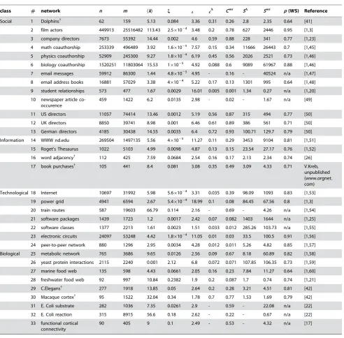
n ð17Þ Table 1.Table of small-world-ness values and other topological properties of real networks.
class # network n m Ækæ j L CD Cws SD Sws p(WS) Reference
Social 1 Dolphins{ 62 159 5.13 0.084 3.36 0.31 0.26 2.8 2.35 0.64 [41]
2 film actors 449913 25516482 113.43 2.561024 3.48 0.2 0.78 627 2446 0.95 [1,3]
3 company directors 7673 55392 14.44 0.002 4.6 0.59 0.88 228 341 0.77 [1,23]
4 math coauthorship 253339 496489 3.92 1.661025 7.57 0.15 0.34 11666 26443 0.7 [1,45]
5 physics coauthorship 52909 245300 9.27 1.861024 6.19 0.45 0.56 2026 2521 0.73 [1,46]
6 biology coauthorship 1520251 11803064 15.53 161025 4.92 0.088 0.6 9089 61967 0.88 [1,46]
7 email messages 59912 86300 1.44 4.861025 4.95 - 0.16 - 40524 n/a [1,47]
8 email address books 16881 57029 3.38 461024 5.22 0.17 0.13 1301 995 0.64 [1,48]
9 student relationships 573 477 1.67 0.0029 16.01 0.005 0.001 1.34 0.27 n/a [1,20]
10 newspaper article co-occurence
459 1422 6.2 0.0135 2.98 - 0.02 - 1.67 n/a [49]
11 US directors 11057 74414 13.46 0.0012 5.19 0.56 0.87 315 494 0.77 [50]
12 UK directors 8850 39741 8.98 0.001 6.46 0.61 0.89 386 561 0.71 [50]
13 German directors 4185 30438 14.55 0.0035 6.4 0.72 0.93 100.71 129.7 0.79 [50]
Information 14 WWW nd.edu 269504 1497135 5.56 461025 11.27 0.11 0.29 3453 9104 0.81 [1,51]
15 Roget’s Thesaurus 1022 5103 4.99 0.0098 4.87 0.13 0.15 23.54 27.17 0.76 [1,52]
16 word adjacency{
112 425 7.59 0.0684 2.54 0.16 0.17 2.13 2.34 0.74 [26]
17 book purchases{
105 441 8.4 0.081 3.08 0.35 0.49 3.09 4.33 0.71 V.Kreb,
unpublished (www.orgnet. com)
Technological 18 Internet 10697 31992 5.98 5.661024 3.31 0.035 0.39 98.09 1093 0.83 [1,53]
19 power grid 4941 6594 2.67 5.461024 18.99 0.1 0.08 84.45 67.56 0.8 [1,3]
20 train routes 587 19603 66.79 0.114 2.16 - 0.69 - 4.26 n/a [1,54]
21 software packages 1439 1723 1.2 0.0017 2.42 0.07 0.082 1403 1644 n/a [1,25]
22 software classes 1377 2213 1.61 0.0023 1.51 0.033 0.012 285.26 103.73 n/a [1,55]
23 electronic circuits 24097 53248 4.42 1.861024 11.05 0.01 0.03 33.5 100.5 0.91 [1,56]
24 peer-to-peer network 880 1296 2.95 0.0034 4.28 0.012 0.011 5.26 4.82 0.85 [1,57]
Biological 25 metabolic network 765 3686 9.65 0.0126 2.56 0.09 0.67 8.18 60.89 0.82 [1,58]
26 yeast protein interactions 2115 2240 0.001 2.12 6.8 0.072 0.071 107.85 106.35 0.73 [1,59]
27 marine food web 135 598 4.43 0.0661 2.05 0.16 0.23 7.84 11.27 0.64 [1,60]
28 freshwater food web 92 997 10.84 0.2382 1.9 0.2 0.087 1.7 0.74 0.74 [1,21]
29 C.Elegans{
277 1918 13.85 0.05 2.64 0.2 0.28 3.21 4.51 0.81 [42]
30 Macaque cortex{
95 1522 32.04 0.34 1.78 0.7 0.77 1.53 1.69 0.79 [42]
31 E. Coli substrate 282 1036 7.35 0.0261 2.9 - 0.59 - 22.08 n/a [22]
32 E. Coli reaction 315 8915 56.6 0.18 2.62 - 0.22 - 0.67 n/a [22]
33 functional cortical connectivity
90 405 9 0.1 2.49 - 0.53 - 4.32 n/a [17]
Entries ‘-’ indicate missing data; n/a indicates values that could not be computed. AllSD,Sws, edge densityjand impliedp(WS) were computed by us; for networks
marked{we have computed some or all ofÆkæ,L,CDandCwsfrom available data-sets. References are given for the source of the original network data, and also for the
analyses where these were done separately. doi:10.1371/journal.pone.0002051.t001
whereh(K,p) is a function ofKandponly. The term in the square brackets tends to 1 asnR‘and so, for large enoughn,SDfor the WS model scales withn. To quantify this approximation, we performed a linear regression on log-transformed quantities (just as for the real networks) over the typical range ofnencountered in our sample of networks, 102
#n#107, and found a linear fit, withr2within 1025of
unity.
Establishing the precise WS model correlate of a real network
The WS network is often used as a generative model for real small-world networks [e.g. 8–13]. This is assumed to establish a ‘first-pass’ model of that system’s topology, which may be augmented by considering other factors such as degree sequence [23], degree correlation [25], modularity [26] and other properties.
In matching the WS parametersK,p,nto the target system, we known, can measureÆkæ (givingK=Ækæ/2), but estimatingphas, hitherto, remained problematic. However, using our new metric of small-world-ness, it is possible to establishpin a principled way. Thus, ifGis a real (target) network with measured small-world-nessSD
g, we identify it with the WS network with the same value of
SD. That is, forme Kð ,p,nÞ~SD
wsðK,p,nÞ{SDg, whereSwsDðK,p,nÞis
given by the right hand side of (17), and minimiseewith respect to p, keeping K, n at their measured values. We did this for our sample of real-world systems, omitting those for whichÆkæ#2 since the expressions used in definingSD
ws are inaccurate in these cases
(we used Matlab routine fzero, initial value of p= 0.5). The resultingpvalues for the equivalent WS model are listed in Table 1 Given that the real-world networks showed SD/n, the WS networks derived from them under the procedure described here must do likewise (they have identical SD values). However, the result in the previous section would suggest that this impliesK,p are roughly constant for this set of WS networks.
To investigate the constancy of K we used the result that Ækæ= 2m/n(wheremis the number of edges in the network). So, using K=Ækæ/2, constant K is equivalent to establishing m/n. Figure 2C shows the result of regressingm againstn(using log-transformed quantities) for the real world networks. For networks
with SD.1, the best fit model was m= 2.46n1.06 (27 networks, r2= 0.92,p= 4610215
), implying a mean node degree ofÆkæ= 2m/ n<5; for networks withSws.1, the best fit model wasm= 3.16n1.03 (30 networks,r2= 0.91,p= 2610215
) implyingÆkæ<6.32. Thus, the real-world networks fulfill the prediction of constant mean node degree. A similar result holds for p values; we found that all testable real-world systems fall into a very limited range ofpfor the equivalent WS model (0.64#p#0.95 andsp= 0.0806).
An alternative view of these results is as follows. We could start with the empirically observed approximate constancy of mean node degreeÆkæand calculated rewiring parameterpfor the real world networks, and deduce a linear scaling of SD for the WS models. Then, under the equivalence ofSD for both real-world networks and their WS counterparts, we could have predicted that SDfor the real-world networks would also scale linearly.
The linear scaling of small-world-ness withnis not inevitable
Is the relationship S/n inevitable for all systems? (The subsequent argument holds for S based on either definition of clustering coefficient and so superscriptsD, ws are dropped). To investigate this we note that it is always possible to writeSi=aini for theith system, for some valueai; in the case of linear scaling,ai is constant. To proceed further, we now expressai in terms of other system parameters. Using the definition of S and (10) for random graphs,
Si~
CiLrand
LiCrand
~Ci
Li
nilnni
SkTilnSkTi ð18Þ
[image:6.612.63.536.60.219.2]whereCi,Li,Ækæiare the clustering coefficient, mean shortest path length, and mean node degree of systemirespectively. While we do not know exactly howLidepends onn, we note that the mean shortest path length for small-world networks is usually assumed to scale logarithmically like random graphs: from (11), Lrand= [1/ ln(Ækæ)]ln(n); and for the WS model, using (9) with largen,Lws= (1/ 4K2p)ln(n). Both relations are of the form L=bln(n) where b is
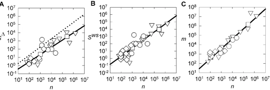
Figure 2. Correlation of real-world network properties. ASmall-world-nessSDscales linearly with network sizenacross real networks from all domains, and irrespective of their other properties. We show SD for all 27 networks for which CDcould be found or calculated; result was SD= 0.023n0.96(r2= 0.78;p= 361029). The dashed line is the theoretical maximum small-world-ness value ofSD= 0.181n(see text), given the implied
mean degree of Ækæ<5 (see below). BSimilarly, using known or calculatedCws, we found Sws= 0.012n1.11(30 networks withSws.1;r2= 0.84;
p= 1.3610211).CNumber of edgesmalso scales linearly with network sizen—CDdata-set shown. Best-fit model wasm= 2.46n1.06(27 networks,
r2= 0.92, p= 4610215), implying a mean node degree of Ækæ= 2m/n<5. For theCws data-set, we found m= 3.16n1.03(30 networks, r2= 0.91,
p= 2610215) implyingÆkæ
<6.32. Residuals of all regressions on log10-transformed data did not significantly differ from a normal distribution at
p= 0.01 (Anderson-Darling test [44].CDdata-set, 27 networks:nvsSD:A2= 0.36,p= 0.5;nvsm:A2= 0.45,p= 0.28.Cwsdata-set, 30 networks:nvsSws:
A2= 0.8,p= 0.04;nvsm:A2= 0.82,p= 0.033). Network domains: social (,); information (); technological (#); biological (X).
doi:10.1371/journal.pone.0002051.g002
independent ofn. We therefore writeLi=biln(ni), wherebiis the factor that ensures the equality to be true (i.e it plays a similar role in this respect asai).
This gives
ai~
Ci
biSkTilnSkTi ð19Þ
In general, there is noa priorireason to suppose that the variables Ci, Ækæi and bi are either all constant, or co-vary in a way commensurate with constancy forai. However, for the sample of networks used here, as noted above, the mean node degreeÆkæiis approximately constant. It is now instructive to see how much co-variation is required between the remaining two variables in order to ensure a significantly different power law holds betweenSandn. Thus, suppose that we fit a modelS=mn1.5so that we expect ai&mn0i:5. For the range ofnencountered here – approximately
four orders of magnitude –aiwould therefore have to range over 2 orders of magnitude. For this to occur, there must be sufficient variation inCi and bi, and these two quantities should correlate well withn. The ranges of the two variables are reasonably large in the data-set – using CD, 0.209#bi#2.52 and 0.005#Ci#0.72 – and could plausibly generate the required 100-fold variation. However, the correlation coefficients withnare very small: forbi, r2= 0.028 and for C
i, r2= 0.025. This would therefore appear to preclude a nonlinear relationship between SD and n for the networks studied here.
To study the effect of a lack of correlation between n and network parameters likeCion linear scaling betweenS
D
andn, we ran a Monte Carlo simulation (see Materials and Methods). Each one of 1000 experiments consisted of sampling 27 randomly drawnCvalues for networks with constantb, and with a spread of nover 4 orders of magnitude. For each network its small-world-ness was computed and a linear regression of S against n performed. This resulted in a mean ofr2= 0.8960.06 s.d. across the 1000 experiments, showing the strong tendency for linearity in this case.
The linear relationship is, however, sensitive to deviations from the approximation that Ækæ is constant. That is, networks that deviate furthest from the linearm/nmodel in turn deviate furthest from the linear S/n model (Figure 3). This was shown using a novel regress-delete-regress procedure outlined in Materials and Methods (we were able to directly test the sensitivity toÆkæ, rather than using a Monte Carlo approach as above, because the strong correlation ofmwithnprovided a baseline from which we could quantify deviation ofÆkæfrom constancy). Further, Figure 3 shows that if we delete a random set of networks from the data-set, then the average effect is to not change the fit to the linearS/nmodel: the linear scaling is robust, and does not depend on a specific network set.
The sensitivity of small-world-ness linearity withnto degreeÆkæ suggests that introduction of networks with very high edge density into our sample would destroy the linear scaling. We can rewrite (8) usingÆkæ= 2m/n
SkT^jn{1, ð20Þ
and see that mean degree scales linearly with edge density. Thus, a network with high edge density implies high mean degree, which in turn would fall far from the linearS=anmodel, as we have just shown.
One exemplar of a real system with high edge density is the network of individual neurons within a single vertebrate brain
region. Detailed network data for these are not available because of the great technical difficulties in reliably reconstructing even small networks such as the 302 neuronC. Elegansnervous system [27]. Indeed, high edge density itself may be the primary cause of technical problems in reconstructing complete systems from many domains, resulting in their absence from the network literature. Nonetheless, approximate reconstructions can be attempted. Quantitative anatomical models of individual brain regions suggest that each of the hundreds of thousands or millions of neurons receive many thousands of connections, and each themselves connect to similar numbers of target neurons [16,28]. Such networks of neurons can have very low small-world-ness values for their size [16], and thus fall far from the linear S/n model discovered here.
We conclude here that the linear relationship between small-world-ness and system size does not hold for an arbitrary collection of networks, but is highly likely if all such networks have a similar mean node degree.
Other scaling properties of small-world-ness
Having established that S scales linearly with n, it is also instructive to look at how its component ratios scale withn. We find, as expected, that most networks falling into the small-world class have approximately the same mean shortest path length as their equivalent E–R random graphs, and sol<1. Given this, it is unsurprising that bothcD
andcws
[image:7.612.317.474.57.204.2]then scale linearly withn(see Figure S1). We did find that three networks in our data-set — email messages (#7), software packages (#21), and software classes (#22) — had l<0.1, indicating that their mean shortest path length was an order of magnitude smaller than the equivalent E–R
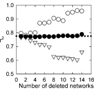
Figure 3. Robustness of WS model predictionS/n.We test the effect of real-world networks deviating from the constant Ækæ
assumption using the following iterative procedure: (i) regressnvsm
for the data-set (as in Figure 2C); (ii) select network to remove from data-set based on regression outcome; (iii) regressnvsSfor reduced data-set and record new goodness-of-fit (asr2); (iv) repeat from (i) until 50% of networks removed. We do this for 3 selection cases, based onSD
here, in step (ii): (a) removing the network with the largest deviation fromm/nlinear model increased the goodness-of-fit (#) for theS/n
linear model (the dotted line indicates the original goodness-of-fit value atr2= 0.78); (b) removing networks with the smallest deviation from
m/nlinear model decreased the goodness-of-fit (,) for theS/nlinear model; (c) random deletion did not consistently change the goodness-of-fit (N). Thus deviation from the assumption of constantÆkæcorrelates
with deviation from the linearS/nmodel for the real-world networks, as predicted by the WS model. In addition, case (c) shows that the linear
S/n model is robust to taking random sub-sets of the networks. Identical trends were obtained forSws. All random deletion data-points averaged over 1000 realizations of the regress-delete-regress sequence; both largest and smallest deviation cases were unique sequences. doi:10.1371/journal.pone.0002051.g003
random graph. These networks are thus ultra-small [29], and indeed both email message (#7) and software package (#21) networks fall further from the linear model than any others.
Given the existence of the linear scaling withn, the scaling of small-world-ness with some other topological properties is completely determined. We can directly determine from (20) how edge density behaves in our data-set (values forjare given in Table 1). Taking our fitted linear modelS=an, we can substitute n=S/ain (20) and find that
S^SkTaj{1:
ð21Þ
Substituting our found values ofÆkæandafor the fits to eitherSws or SD confirms that this is a good approximation. Therefore, because small-world-ness linearly scales with network size, and degree is approximately constant, thenSalso has a simple inverse linear scaling with edge density.
Real-world systems do not maximize small-world-ness
We can show that the specific scaling coefficient a in the relationship S=anfor the real-world networks studied here does not maximize small-world-ness for a particular size of network. First, we show that the WS model predicts an approximately constant amount of rewiringpthat maximizesSD, independent of network size. To do this, given the above analytic expressions (13) forlwsand (16) forcDws(and again assumingnKp&1), we found dSD
ws
dp, and setdSD
ws
dp~0. Solving this equality forpwould then give us the value ofpthat maximizedSD
ws, if one existed —
see Text S1 for details of the solution.
We did this over the rangen[103,1020 withK=Ækæ/2 = 2.5,
since this is implied by the result of Figure 2C. Ifp*is the value ofp giving maximal SD
ws, we found that for small networks (n= 10 3
) p*= 0.222 and, asnR‘,p*R0.246, so that the range ofp*is very
small. The constantKand very small range ofp*imply that the associated maximum SD
ws values should scale linearly with n. It
transpires that the theoretical maximum SDws depends almost
exactly in a linear way on n with slope 0.181 (and plotted in Figure 2A). Thus,SDis not maximized by the real-world networks.
A generative mechanism for a specific linearS/n
relationship
We have established and explained many simple properties of real-world networks and of their equivalence class in the WS model. We now show how the specific, sub-maximal, linear scaling ofS=ancould have been generated. The models we examine here are intended as informative examples of the generation and limits onSscaling, not an exhaustive list of those which could generate the specific linear scaling we found — that remains the subject of future work.
Many of the real-world systems share common generative principals despite their widely differing origins. Most systems have a growth process, showing some form of preferential attachment [30] that is limited by the cost of adding new edges and by the capacity to maintain them (as might be induced by aging) [31]. Simple models of this process result in ‘scale-free’ networks with power-law or truncated power-law degree distributions [30,31], a property that is also common to many real-world systems considered here [32] (but see [33] for an alternative view of some biological networks). However, networks generated by these models are not ‘small-world’ by either Definition 1 or 2. Their clustering coefficient is inversely proportional ton, going to zero as ngrows large [34]. Thus, they cannot show linear scaling ofS: it is at best constant and at worst goes to zero with increasingn.
A noisy, limited growth processcangenerate the specific linear S=anrelationships we report. A generalized form of the Klemm-Eguiluz model (GKE)[34,35] encapsulates this process, and has the unique property of creating networks that are both small-world (short path length, high clustering) and ‘scale-free’ (having a truncated power-law degree distribution) as found for many real-world systems considered here. (To the best of our knowledge, all known real-world systems with power-law-like degree distributions also fall into the broad ‘small-world’ class we discussed in the Introduction; it is only the scale-free networks formed by the simple models that form a distinct set of ‘scale-free-only’ networks). By using the GKE model, we therefore also show that linear scaling ofScan occur whether or not the real-world systems have ‘scale-free’ properties.
The GKE model begins with an active set ofMnodes. At every time-step a new node is added, connecting d edges: one edge added to a random inactive node with probabilityr, adding noise to the process; all remaining edges connect to randomly chosen active nodes. One of the active nodes is deactivated with a probability proportional to the active nodes’ degrees; finally, the new node is activated. The sequence repeats until the desired size of network is obtained.
We found that specific values forMandrcould generate GKE networks with the same linear scaling relationships between network size andSwsandSDthat we observed for the real-world networks (Figure 4; see Materials and Methods, and Figure S2). Therefore, a possible general mechanism for particular linear scaling rates of small-world-ness is a common size of both active node set and quantity of noise during creation of the real-world systems.
Discussion
[image:8.612.315.471.477.603.2]Small-world-ness is a topological property linking real-world systems across domains of research. Hitherto it has been defined only in semi-quantitative way (Definition 1). In this paper we propose quantitative measures of small-world-ness –SDandSws– and define a network to be in the small-world category with respect to either of them if the small-world-ness is greater than 1
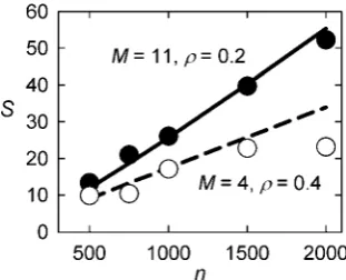
Figure 4. A limited growth process can generate the observed S/n relationships. We created 5 networks for every value of
n[½500,750,1000,1500,2000 using a generalized form of the
Klemm-Eguiluz model (GKE) [34,35], settingd= 3 so that the resulting networks had the same mean degree (,6) as we found for the real-world
systems. We searched on the GKE model’sMandrparameters (see text) to minimize the root mean square error between the resulting scaling of the averagedSws(N) andSD(#) values and the observed
real-world network relationships (respectively, the solid and broken lines). The best-fit parameters were different for the two forms of S, underlining that they measure two different properties of the real systems.
doi:10.1371/journal.pone.0002051.g004
(e.g Definition 2). This quantification of small-world-ness allows for the statistical testing of its presence in any given network.
The Watts-Strogatz (WS) model plays a key role in the study of small-world networks. It uses a generative process to create classes of small-world network and is now widely used as a model for studying dynamic systems [3–13]. However, until now, a precise parameterization of the WS model associated with a given kind of real-world network remained elusive. Our introduction of a quantitative measure of small-world-ness remedies this by demanding that the WS counterpart to a specific network have the same value ofSD(orSws). For the WS models it is possible to show analytically that, under certain circumstances (constant re-wiring parameter and range), the small-world-ness SDwill scale linearly with network sizen. Intriguingly, a wide class of real-world networks also shows this linear scaling. Given this similarity in behavior, the assumption of (limited) topological correspondence of the WS model with real networks implies certain constraints on empirically measured parameters (like mean degree) of these networks. These constraints appear to hold, and so the ideas developed here provide further support for using the WS model in the study of small-world systems.
We have shown that the linear scaling betweenSDandnis not an inevitable property of networks; it would be possible, for example, to include networks with very large edge density that would destroy any linear scaling. However, in the event of linear scaling, there is a variety of possible scaling constants and there is a noisy growth process that could give rise to the networks sharing the same scale (slope) parameter. Finally, we have shown that the small-world networks used here do not maximize SD (there are ‘steeper’ linear relationships betweenSDandn).
We cannot, on the basis of the work presented here, answer the question of why small-world-ness was not maximised, but we can give some insights as to why this is the case. The possible explanations split into two broad classes of structural and dynamical limitations. Our use of the GKE model showed that the limited capacity of a system’s nodes to maintain edges (whether due to physical cost, aging processes, or some other mechanism) is one structural limitation that could result in sub-maximal small-world-ness. Other structural limitations could include physical limits on node location and length of edges, such as might occur for the sub-stations and transmission wires in the power grid network.
Even if structural limitations were not an issue, then the system may have dynamical requirements that prevent it from maximis-ing small-world-ness. The constraints placed on a system’s topology by the dynamics required to fulfill its function are not well understood. Recent work has shown how the presence of particular network ‘motifs’ — repeating patterns of connections between a small number of nodes — can guarantee, for example, a chaotic attractor for the network as a whole [36]. The functional requirements of some real-world system may then lead to the inclusion of particular motifs to guarantee the necessary dynamics [37], and there is no necessary link between a system’s motifs and its global topological properties (of which small-world-ness is but one). Nonetheless, given that so many of the key motifs identified so far are either complete 3-node loops or contain them [37,38], the global topology will have a high clustering coefficient, and will most likely be a small-world network.
Other systems may have constraints placed directly on their global topology, and this too could prevent maximisation of world-ness. For example, in his original work on the small-world model, Watts [39] explored the dynamics of Kuramoto oscillators on a WS model substrate, and showed that the fraction of synchronised oscillators had a phase transition that
occurred for progressively smallerpas the oscillators’ symmetric coupling strength increased (for fixed n, K). Therefore, if a system’s function required it to be at the phase transition, so that it could rapidly switch between synchronised and desynchronised states with minimal perturbation, the required amount of (implied) rewiring may be far from that which maximised small-world-ness.
These are just a few of many possible explanations for why real-world systems do not maximise small-real-world-ness. Instead we might ask, when would small-world-ness be maximised? Maximum S essentially identifies the point in the network’s possible topologies where the highest clustering is achieved for the smallest deviation from the shortest mean path length. Such a network would be optimal for message-passing, such that all the nodes receive a message in the shortest possible number of network steps [40]. On this basis, we expect that some form of dynamic phenomenon, whether based on percolation (or, equivalently, epidemiological SIR models), oscillators, or some other general ordinary differential equation system, will have a strong correlation with small-world-ness. So, just as we have used a continuously graded ‘small-world-ness’ to quantitatively examine the topologies of the broad class of small-world networks, we may use this as the starting point for quantifying the continuum of dynamic properties that must also span this class.
Materials and Methods
Data-set of real-world systems
We collated a database of real-world networks’ topological properties, combining published results with our own analyses of available data-sets. These are presented in Table 1, extending the previous considerable effort of collating topological properties by Mark Newman [1]. All networks are treated as undirected. We list 33 real-world systems in total: we could computeSwsfor all systems andSDfor 27 systems —CDcould not be found or computed for those systems.
We emphasise that the networks were not chosen for their ability to fit the linear model ofS/n. The majority of the data-set (21 of 33) were obtained from a previous collation [1]: networks were only omitted from that prior data-set if neitherCwsorCDwere available for them (and hence were of no practical use to us here). Many of the additional networks we added filled sub-domains missing from the prior data-set, for example: the dolphin network [41] is an example of an animal social network; the cortical area connectivity map [42] is an example of large-scale neural connectivity. In addition, the regress-delete-regress sequence we used in the main text (and see below) shows two properties. First, that we could have applied that method to the data-set in Table 1 before further analysis, pruning the data-set down to those networks that showed the best fit to the linear model (by choosing the ‘most-deviant’ networks to omit), but did not. Second, that the linear scaling property is robust across randomly chosen sub-sets of the network data-set: on average, randomly deleting networks from the data-set did not significantly reduce the fit to the linear model.
Testing significance ofSscores
We assess the significance of borderline small-world-ness scoresS1 using Monte Carlo methods. The null hypothesis for the Watts-Strogatz definition of small-world networks is that the system is an Erdo¨s-Re´nyi (E–R) random graph. We thus constructedN= 1000 E–R networks with the same number of nodes n and edges m for each tested real-world system, computing SD
i and Swsi for the ith E–R network. The 99%
confidence limits for the null hypothesis were then defined for
each system. We first found the central 99% interval [a*, b*], that is [43]
# SD
iva
N ~0:005,
# SD
ivb
N ~0:995, ð22Þ
and similarly forSws. The 99% confidence interval for the system is then
CI~b {a
2 : ð23Þ
The upper 99% confidence limit is then CL0.01 = 1+CI (where by definitionSws,SD= 1 for an E–R random graph). A network with S.CL0.01 was therefore considered to significantly differ from a random network. We note that adopting a quantitative definition (Definition 2) of small-world-ness has led us to a procedure for a general statistical test for the presence of small-world structure, as defined by Watts and Strogatz [3], which is particularly useful for establishing meaningful departures from randomness in small networks.
Fits to linear scaling
Least-squares regressions on small-world-ness S and number of edges m against size of system n were performed on log10
-transformed data to normalize magnitude of errors across range ofn. Best fit linear model log10(x) =a+blog10(n) back-transformed
to a linear basis, giving x=anb, where a= 10a and b=b. MATLAB (Mathworks) functionregress was used to perform the regressions. The validity of r2 significance values was established by confirming that the residuals of each regression had a normal distribution atp= 0.01 using the Anderson-Darling test [44].
A regress-delete-regress procedure for testing robustness of predictions
We test the effect of real-world networks deviating from the constantÆkæassumption using the following iterative procedure:
1. regressnvsmfor the data-set (as in Figure 2B);
2. select network to remove from data-set based on regression outcome (3 different selection criteria were used, detailed below);
3. regressnvsSfor reduced data-set and record new goodness-of-fit (asr2);
4. repeat from step 1 until 50% of networks removed.
We do this for 3 selection cases in step 2. First, we tested removing the network with the largest deviation fromm/nlinear model in each iteration, hypothesizing that this should lead to an overall increase in fit to a linear model (increasedr2) forS=f(n) if the WS model behaviour reflected that of real-world systems. Second, we tested removing the network with the smallest deviation fromm/nlinear model at each iteration, hypothesizing that this should lead to an overall decrease in fit to a linear model (decreasedr2) forS=f(n) if the WS model behaviour reflected that of real-world systems. Third, we tested random deletion, where a random network was deleted at each iteration, irrespective of the regression outcome, to establish the baseline effect of removing systems from the data-set. The first and second cases are unique sequences of deleted networks; the third case we repeated 1000 times.
Monte Carlo testing of linear scaling
We tested the dominance of linear S/n scaling given an approximately constant mean node degree Ækæ and path length scalingb. For each Monte Carlo simulation, we drew 27 random Cvalues from a uniform distribution in [0,1], computing ai for each from Eq. (19) with constant bi= 1 and Ækæi= 6. We then computed Si=aini for each, using a logarithmic spread of 27 network sizesn[102,106to closely match the spread of the
real-world system sizes. Linear regression (as detailed above, including the log10-transform) was then performed on the set of simulated 27 Svalues and the r2 recorded. We repeated this procedure 1000 times.
Searching GKE model parameter space
We wished to determine if the generalized Klemm-Eguiluz model (GKE)[31,32] model could explain the particular scaling relationships we found for the real-world systems:
SD~0:023n0:96, ð24Þ
Sws~0:012n1:11: ð25Þ
We explored the (M, r) parameter space, searching over
M[½3,30in steps of 1, andr[½0,0:5in steps of 0.1. The lower
limit onMis set by the number of edges added per new vertex, and here we setd= 3 to give a mean degree ofÆkæ<6 for a GKE model network, approximately the same degree that was implied by the linearm/nrelationship for the real-world systems. For each (M,r) pair, we constructed 5 GKE model networks for each value of n[½500,750,1000,1500,2000and computed their Sws and SD
scores. We took the mean of these 5 scores for eachn, giving sets
S Sws
500,SSws750,SS1000ws ,SSws1500,SSws2000
and SSD
500,SSD750,SS1000D ,SSD1500,SS2000D
. The fit of the GKE model networks was then assessed by computing the root mean square error (RMSE) between these mean values and those given by the scaling relationships (24) and (25) for the tested sizes of network n. The parameters that minimised RMSE are given in Figure 4; the error landscapes are shown in Figure S2.
Supporting Information
Text S1 Supporting information text
Found at: doi:10.1371/journal.pone.0002051.s001 (0.22 MB PDF)
Figure S1 Correlation of real-world systems’ clustering coeffi-cient and path length ratios with system size. Clustering coefficoeffi-cient ratios (a)cD=CDCrandand (b)cws=CwsCrandboth scaled linearly
with S. Linear regressions found r2>0.86 in both cases. (c) As expected for small-world-networks, path length L was approxi-mately the same as that of an E-R random graph, and sol=L/ Lrand1 for most networks (note that we show l here for all 33
networks). All linear regressions performed on log10-transformed
data, as detailed in Materials and Methods of the main text. Found at: doi:10.1371/journal.pone.0002051.s002 (0.11 MB TIF)
Figure S2 The root mean square error (RMSE) distribution across tested values of the GKE model parameters. The RMSE is computed based on the difference between the mean values of small-world-ness for a set of generated GKE networks and the corresponding small-world-ness values from the specific linear relationships found for the real-world systems. (a) RMSE error
distribution for the fit to theSws/nrelationship. RMSE plotted on log scale to emphasise valley of minimum values. Stick-and-ball indicates the parameter pair that minimised RMSE. (b) RMSE error distribution for the fit to theSD/nrelationship. Stick-and-ball indicates the parameter pair that minimised RMSE. Found at: doi:10.1371/journal.pone.0002051.s003 (0.44 MB TIF)
Acknowledgments
We thank M. Newman and M. Kaiser for making their data-sets publicly available, and T. Stafford and T. Prescott for comments on drafts of this manuscript.
Author Contributions
Conceived and designed the experiments: MH KG. Performed the experiments: MH. Analyzed the data: MH KG. Contributed reagents/ materials/analysis tools: MH. Wrote the paper: MH KG.
References
1. Newman MEJ (2003) The structure and function of complex networks. SIAM Review 45: 167–256.
2. Boccaletti S, Latora V, Moreno Y, Chavez M, Hwang DU (2006) Complex networks: Structure and function. Phys Rep 424: 175–308.
3. Watts DJ, Strogatz SH (1998) Collective dynamics of ‘small-world’ networks. Nature 393: 440–442.
4. Lago-Fernandez LF, Huerta R, Corbacho F, Siguenza JA (2000) Fast response and temporal coherent oscillations in small-world networks. Phys Rev Lett 84: 2758–2761.
5. Barahona M, Pecora LM (2002) Synchronization in small-world systems. Phys Rev Lett 89: 054101.
6. Nishikawa T, Motter AE, Lai YC, Hoppensteadt FC (2003) Heterogeneity in oscillator networks: are smaller worlds easier to synchronize? Phys Rev Lett 91: 014101.
7. Roxin A, Riecke H, Solla SA (2004) Self-sustained activity in a small-world network of excitable neurons. Phys Rev Lett 92: 19801.
8. Little LR, McDonald AD (2007) Simulations of agents in social networks harvesting a resource. Ecol Model 204: 379–386.
9. Janssen MA, Jager W (2001) Fashions, habits and changing preferences: Simulation of psychological factors affecting market dynamics.
10. Delre S, Jager W, Janssen M (2007) Diffusion dynamics in small-world networks with heterogeneous consumers. Comput Math Organ Theory 13: 185–202. 11. Keeling MJ, Eames KTD (2005) Networks and epidemic models. J R Soc
Interface 2: 295–307.
12. Saramaki J, Kaski K (2005) Modelling development of epidemics with dynamic small-world networks. J Theor Biol 234: 413–421.
13. Netoff TI, Clewley R, Arno S, Keck T, White JA (2004) Epilepsy in small-world networks. J Neurosci 24: 8075–8083.
14. Newman ME, Moore C, Watts DJ (2000) Mean-field solution of the small-world network model. Phys Rev Lett 84: 3201–3204.
15. Bollobas M (2001) Random Graphs, 2nd Edition. Cambridge: Cambridge University Press.
16. Humphries MD, Gurney K, Prescott TJ (2006) The brainstem reticular formation is a small-world, not scale-free, network. Proc Biol Sci 273: 503–511. 17. Achard S, Salvador R, Whitcher B, Suckling J, Bullmore E (2006) A resilient, low-frequency, small-world human brain functional network with highly connected association cortical hubs. J Neurosci 26: 63–72.
18. Bassett DS, Meyer-Lindenberg A, Achard S, Duke T, Bullmore E (2006) Adaptive reconfiguration of fractal small-world human brain functional networks. Proc Natl Acad Sci USA 103: 19518–19523.
19. Sporns O (2006) Small-world connectivity, motif composition, and complexity of fractal neuronal connections. Biosystems 85: 55–64.
20. Bearman PS, Moody J, Stovel K (2004) Chains of affection: The structure of adolescent romantic and sexual networls. Am J Sociol 110: 44–91.
21. Martinez ND (1991) Artifacts or attributes? effects of resolution on the Little Rock Lake food web. Ecol Monogr 61: 367–392.
22. Wagner A, Fell DA (2001) The small world inside large metabolic networks. Proc Biol Sci 268: 1803–1810.
23. Newman ME, Strogatz SH, Watts DJ (2001) Random graphs with arbitrary degree distributions and their applications. Phys Rev E 64: 026118. 24. Barrat A, Weigt M (2000) On the properties of small-world networks. Eur
Phys J B 13: 147–160.
25. Newman ME (2003) Mixing patterns in networks. Phys Rev E 67: 026126. 26. Newman MEJ (2006) Finding community structure in networks using the
eigenvectors of matrices. Phys Rev E 74: 036104.
27. White JG, Southgate E, Thomson JN, Brenner S (1986) The structure of the nervous system of the nematode wormCaenorhabditis Elegans. Phil Trans Roy Soc B 314: 1–340.
28. Braitenberg V, Schuz A (1998) Cortex: Statistics and Geometry of Neuronal Connectivity. Berlin: Springer, 2nd edition .
29. Cohen R, Havlin S (2003) Scale-free networks are ultrasmall. Phys Rev Lett 90: 058701.
30. Barabasi AL, Albert R (1999) Emergence of scaling in random networks. Science 286: 509–512.
31. Amaral LA, Scala A, Barthelemy M, Stanley HE (2000) Classes of small-world networks. Proc Nat Acad Sci USA 97: 11149–11152.
32. Newman MEJ (2005) Power laws, Pareto distributions and Zipf’s law. Contemporary Physics 46: 323–351.
33. Khanin R, Wit E (2006) How scale-free are biological networks. J Comput Biol 13: 810–818.
34. Klemm K, Eguiluz VM (2002) Growing scale-free networks with small-world behavior. Phys Rev E 65: 057102.
35. Tian L, Zhu CP, Shi DN, Gu ZM, Zhou T (2006) Universal scaling behavior of clustering coefficient induced by deactivation mechanism. Phys Rev E 74: 046103.
36. Zhigulin VP (2004) Dynamical motifs: building blocks of complex dynamics in sparsely connected random networks. Phys Rev Lett 92: 238701.
37. Milo R, Itzkovitz S, Kashtan N, Levitt R, Shen-Orr S, et al. (2004) Superfamilies of evolved and designed networks. Science 303: 1538–1542.
38. Prill RJ, Iglesias PA, Levchenko A (2005) Dynamic properties of network motifs contribute to biological network organization. PLoS Biol 3: e343.
39. Watts DJ (1999) Small Worlds: The Dynamics of Networks Between Order and Randomness. Princeton: Princeton University Press.
40. Latora V, Marchiori M (2001) Efficient behaviour of small-world networks. Phys Rev Lett 87: 198701.
41. Lusseau D (2003) The emergent properties of a dolphin social network. Proc Biol Sci 270 Suppl 2: S186–S188.
42. Kaiser M, Hilgetag CC (2006) Nonoptimal component placement, but short processing paths, due to long-distance projections in neural systems. PLoS Comput Biol 2: e95.
43. Efron B (1979) Computers and the theory of statistics: Thinking the unthinkable. SIAM Review 21: 460–480.
44. Stephens MA (1974) EDF statistics for goodness of fit and some comparisons. J Am Stat Assoc 69: 730–737.
45. de Castro R, Grossman JW (1999) Famous trails to Paul Erdos. Math Intelligencer 21: 51–63.
46. Newman ME (2001) The structure of scientific collaboration networks. Proc Natl Acad Sci USA 98: 404–409.
47. Ebel H, Mielsch LI, Bornholdt S (2002) Scale-free topology of e-mail networks. Phys Rev E 66: 035103.
48. Newman MEJ, Forrest S, Balthrop J (2002) Email networks and the spread of computer viruses. Phys Rev E 66: 035101.
49. Ozgur A, Bingol H (2004) Social network of co-occurrence in news articles. In: Aykanat C, Dayar T, Korpeoglu I, eds. Computer and Information Sciences -ISCIS 2004. Berlin: Springer, volume LNCS3280, pp 688–695.
50. Conyon MJ, Muldoon MR (2006) The small world of corporate boards. J Bus Finan Account 33: 1321–1343.
51. Albert R, Jeong H, Barabasi AL (1999) Diameter of the world-wide web. Nature 401: 130–131.
52. Knuth DE (1993) The Stanford GraphBase: A Platform for Combinatorial Computing Addison-Wesley, Reading, MA.
53. Faloutsos M, Faloutsos P, Faloutsos C (1999) On power-law relationships of the internet topology. Comput Commun Rev 29: 251–262.
54. Sen P, Dasgupta S, Chatterjee A, Sreeram PA, Mukherjee G, et al. (2003) Small-world properties of the Indian railway network. Phys Rev E 67: 036106. 55. Valverde S, Ferrer Cancho R, Sole´ RV (2002) Scale-free networks from optimal
design. Europhys Lett 60: 512–517.
56. Cancho RF, Janssen C, Sole` RV (2001) Topology of technology graphs: small world patterns in electronic circuits. Phys Rev E 64: 046119.
57. Adamic LA, Lukose RM, Puniyani AR, Huberman BA (2001) Search in power-law networks. Phys Rev E 64: 046135.
58. Jeong H, Tombor B, Albert R, Oltvai ZN, Baraba´si AL (2000) The large-scale organization of metabolic networks. Nature 407: 651–654.
59. Jeong H, Mason SP, Barabasi AL, Oltvai ZN (2001) Lethality and centrality in protein networks. Nature 411: 41–42.
60. Huxham M, Beaney S, Raffaelli D (1996) Do parasites reduce the chances of triangulation in a real food web? Oikos 76: 284–300.