Nonlinear hydrodynamical evolution of eccentric Keplerian discs in two dimensions: validation of secular theory

discs in two dimensions: validation of secular theory

.

White Rose Research Online URL for this paper:

http://eprints.whiterose.ac.uk/108971/

Version: Accepted Version

Article:

Barker, AJ and Ogilvie, GI (2016) Nonlinear hydrodynamical evolution of eccentric

Keplerian discs in two dimensions: validation of secular theory. Monthly Notices of the

Royal Astronomical Society, 458 (4). pp. 3739-3751. ISSN 0035-8711

https://doi.org/10.1093/mnras/stw580

[email protected]

Reuse

Unless indicated otherwise, fulltext items are protected by copyright with all rights reserved. The copyright

exception in section 29 of the Copyright, Designs and Patents Act 1988 allows the making of a single copy

solely for the purpose of non-commercial research or private study within the limits of fair dealing. The

publisher or other rights-holder may allow further reproduction and re-use of this version - refer to the White

Rose Research Online record for this item. Where records identify the publisher as the copyright holder,

users can verify any specific terms of use on the publisher’s website.

Takedown

If you consider content in White Rose Research Online to be in breach of UK law, please notify us by

Nonlinear hydrodynamical evolution of eccentric Keplerian

discs in two dimensions: validation of secular theory

A. J. Barker

_{and G. I. Ogilvie}

Department of Applied Mathematics and Theoretical Physics, University of Cambridge, Centre for Mathematical Sciences, Wilberforce Road, Cambridge CB3 0WA, UK

ABSTRACT

We perform global two-dimensional hydrodynamical simulations of Keplerian discs with free eccentricity over thousands of orbital periods. Our aim is to determine the validity of secular theory in describing the evolution of eccentric discs, and to explore their nonlinear evolution for moderate eccentricities. Linear secular theory is found to correctly predict the structure and precession rates of discs with small eccentricities. However, discs with larger eccentricities (and eccentricity gradients) are observed to precess faster (retrograde relative to the orbital motion), at a rate that depends on their eccentricities (and eccentricity gradients). We derive analytically a nonlinear secular theory for eccentric gas discs, which explains this result as a modification of the pressure forces whenever eccentric orbits in a disc nearly intersect. This effect could be particularly important for highly eccentric discs produced in tidal disruption events, or for narrow gaseous rings; it might also play a role in causing some of the variability in superhump binary systems. In two dimensions, the eccentricity of a moderately eccentric disc is long-lived and persists throughout the duration of our simulations. Eccentric modes are however weakly damped by their interaction with non-axisymmetric spiral density waves (driven by the Papaloizou-Pringle instability, which occurs in our idealised setup with solid walls), as well as numerical diffusion.

Key words: accretion, accretion discs – planetary systems – hydrodynamics – waves – instabilities

1 INTRODUCTION

Eccentric gas discs are thought to arise in a number of as-trophysical contexts. The orbital evolution of a newly born planet due to its tidal interaction with the protoplanetary disc is intricately coupled with the evolution of eccentric motions within the disc. But the importance of this inter-action in producing the eccentricities of observed exoplan-ets is currently unclear (Papaloizou et al. 2001; Papaloizou 2002; Goldreich & Sari 2003; Kley & Dirksen 2006; D’Angelo et al. 2006; Bitsch et al. 2013). Eccentric gas discs are also thought to explain the superhump phenomenon in SU UMa-type binary stars (Whitehurst 1988; Lubow 1991; Goodchild & Ogilvie 2006; Smith et al. 2007) and the spectral variabil-ity of rapidly rotating Be stars (Okazaki 1991; Papaloizou et al. 1992; Ogilvie 2008). In addition, eccentric gas discs are formed by the tidal disruption of stars or gaseous plan-ets (Guillochon et al. 2011; Liu et al. 2013; Guillochon et al. 2014), and such a process might be responsible for the gas cloud G2 near Sgr A* in the Galactic Centre (Guillochon et al. 2014; Coughlin & Nixon 2015; Pfuhl et al. 2015).

De-⋆ _{Email address: [email protected]}

spite this wide range of applications, the nonlinear dynamics of eccentric discs remains poorly understood.

In the Solar system, several of the rings of Saturn and Uranus are observed to be elliptical, and a theory for nar-row eccentric rings (with small eccentricities but arbitrary eccentricity gradients) composed of weakly collisional par-ticles has been developed (Borderies et al. 1983; Chiang & Goldreich 2000). For small eccentricities, eccentric discs can be described as slowly precessing one-armed density waves (or shocks) (e.g. Okazaki 1991; Papaloizou et al. 1992; Lee & Goodman 1999; Goodchild & Ogilvie 2006; Ogilvie 2008; Saini et al. 2009). A particular solution for a global uni-formly eccentric (and apsidally aligned) Keplerian disc has also been studied by Statler (2001).

pro-portional to the planet-to-star mass ratio; secular theory ac-counts for the long-term behaviour of eccentricity and incli-nation resulting from the orbit-averaged perturbing forces. For a thin gaseous disc around a star, however, pressure pro-vides the most important departure from Keplerian orbital motion, being of second order in the aspect ratio H/R of the disc. Other subdominant forces, such as those due to the self-gravity of the disc (Tremaine 2001) and viscous or turbulent stresses (Ogilvie 2001), can also be important. In this situation, secular theory describes the long-term evolu-tion of eccentricity due to gas pressure (and other forces) in thin discs, but neglects contributions that are of fourth order or higher inH/R.

In recent work, we developed a local model of an ec-centric disc (Ogilvie & Barker 2014), which is similar to the shearing box that is commonly used to study the dynam-ics of circular astrophysical discs (Goldreich & Lynden-Bell 1965; Hawley et al. 1995). We used this model to analyse the vertical oscillatory flows that are driven by the variation in the vertical gravity around a non-circular orbit (Ogilvie & Barker 2014), and subsequently studied the local linear stability of these discs and their vertical flows (Barker & Ogilvie 2014). We found that eccentric discs are generically unstable (in three dimensions), being subject to a small-scale instability in which inertial waves are driven by a parametric resonance. This instability is expected to lead to wave ac-tivity or turbulence, and to damping of the disc eccentricity and eccentricity gradients (Papaloizou 2005b), unless these are maintained by external forcing (or additional instabili-ties e.g. viscous overstability). Nonlinear simulations are re-quired to determine the efficiency of this damping process so that its importance in real discs can be quantified (e.g. con-tinuing the work begun by Papaloizou 2005b, by taking into account the vertical structure of the disc).

In this paper we study the nonlinear hydrodynamical evolution of eccentric discs in two dimensions, deferring three-dimensional simulations to future work. Our aim is to determine the validity of linear secular theory (Ogilvie 2001; Papaloizou 2002; Ogilvie & Barker 2014) in describ-ing the structure and precession rates of eccentric discs, as well as to determine their two-dimensional nonlinear dynam-ics. In the process, we will derive analytically, and compare with simulations, a two-dimensional nonlinear secular the-ory for isothermal eccentric discs that is valid for any eccen-tricity and ecceneccen-tricity gradient, for a thin untwisted disc with non-intersecting orbits – this is a particular case of the general theory of Ogilvie (2001) that is amenable to analyt-ical study. In two dimensions, eccentric discs do not exhibit the parametric instability or vertical oscillatory flows. How-ever, a fundamental study of the two-dimensional nonlinear dynamics of eccentric discs has not yet been undertaken. We believe this to be worthwhile, in spite of the clear im-portance of three-dimensional effects in reality, because the two-dimensional dynamics that we will study are likely to also play a role in three dimensions. In particular, the force due to gas pressure, which tends to cause retrograde pre-cession of these discs, can be captured in two dimensions. These simulations also provide a necessary benchmark to al-low comparison with future three-dimensional simulations.

We outline our intentionally simplified numerical setup designed to study the dynamics of eccentric discs in§2. We derive analytically a nonlinear secular theory for untwisted

eccentric discs in two-dimensions in Appendix A. This the-ory is explored, and its predictions for the shapes and preces-sion rates of eccentric discs are compared with simulations, in§3. The long-term nonlinear evolution of eccentric discs is presented in §4, where we also analyse the background instability that arises due to our idealised setup with rigid walls in the absence of any free eccentricity. We then finish with our conclusions.

2 SIMPLIFIED MODEL

2.1 Background disc

Our model consists of an eccentric (nearly) Keplerian disc in a two-dimensional cylindrical domain as an initial condition. We study its resulting nonlinear evolution using the PLUTO code (Mignone et al. 2007), adopting cylindrical polar coor-dinates (R, φ) with corresponding velocity componentsuR

anduφ. Our governing equations are

(∂t+u· ∇)u=−1 Σ∇p−

GM

R2 eR, (1)

∂tΣ +∇ ·(Σu) = 0. (2)

To allow us to more easily understand the outcome of our simulations, we consider a power-law disc which is isother-mal (where the pressurep=c2

sΣ, and Σ is the total surface

density; with sound speedcs= const), with background disc

surface density,

Σb(R) = Σ0R−σ, (3)

for the circular case, whereσwill be varied. (We expect the qualitative results of this paper to carry over to discs with different thermodynamic behaviour, and those with a ra-dially varying sound speed.) The axisymmetric basic state of the disc has angular velocity Ω = Ω0R−

3

2 (which does

not strictly apply whenσ6= 0 due to radial pressure gradi-ents), where Ω0is the Keplerian angular velocity atR=Ri,

anduφ=RΩ. Our disc occupies the full azimuthal extent1

φ∈[0,2π), with radial extentR∈[Ri, Ro], on which the

ra-dial boundary conditions are “reflecting” conditions2_{. These}

boundary conditions were chosen to confine the eccentric disc for a well-defined study. While these are not appropri-ate for all applications in which eccentric discs are thought to arise, they may reasonably approximate the boundaries of a disc that has been tidally truncated (e.g. Papaloizou 2005b). For example, our model might be relevant to nar-row rings that may be produced by disc-planet interactions that have formed multiple gaps. A reflecting edge may also be appropriate to describe the inner edge of the disc, if there is a sharp drop in the density there, or where discs match onto the surfaces of central objects e.g. white dwarfs

1 _{Meaning that periodic boundary conditions are applied to all}

quantities atφ= 0 andφ= 2π.

2 _{This means that the radial velocity in the ghost cells adjacent}

in Cataclysmic Variable systems. However, the aim of this paper is not to focus on any particular application, but to explore the fundamental dynamics of eccentric discs that might have more general applicability. We choose units such that Ω0 = Ri = Σ0 = 1, and vary the parameters cs (to

mimic a disc with aspect ratio H/R ∈ [0.025,0.1]),σ and

Ro, in addition to the eccentricity of the disc, which we will

now describe.

2.2 Eccentric mode

We initialise an eccentric disc using nonlinear secular the-ory (Appendix A). To do this we modify the velocity com-ponents and surface density of the background disc so that they describe an eccentric mode, to make the streamlines elliptical. The eccentric mode is a global slowly precessing density wave that satisfies the boundary conditions.

We define the complex eccentricityE(λ) =e(λ)eiω(λ), whereeandωare the eccentricity and longitude of pericen-tre. In secular theory, orbits are labelled using their semi-latus rectumλ, related to cylindrical radius by

R(λ, φ) = λ

1 +e(λ) cos (φ−ω(λ)). (4)

In linear secular theory for a 2D isothermal disc,

2Σ GM λ3

1

2_∂

tE= ic2s ∂λ Σλ3E′+λ2E∂λΣ, (5)

where E′ _≡∂

λE, and in this case R and λ are equivalent

(this can be transformed into the Schr¨odinger equation). Eq. A10 is the equivalent equation in the nonlinear secu-lar theory of Appendix A (in which care must be taken to take into account the difference between R andλ, and the resulting equation is a type of nonlinear Schr¨odinger equa-tion). We seek solutions that precess at the rate ωp, such

thatE∝eiωpt_{. Together with the boundary conditions}

E(λi) =E(λo) = 0, (6)

appropriate for fixed circular boundaries, we obtain an eigenvalue problem for the eigenvalueωp and eigenfunction

E. We solve this problem using a shooting method (Press et al. 1992), which works equally well for the solution of Eq. A10 (which is a nonlinear equation forE andE′_{). This}

method requires us to provide an initial guess for ωp and

E′_(λ

i) to select the appropriate solution. To do this, we use

a combination of trial and error and the results of an in-dependently coded solution to the linear problem using a Chebyshev collocation method. In each case, we select the fundamental eccentric mode, which has a single maximum in the eccentricity. This is the slowest precessing mode with the longest radial wavelength, which is chosen because it can be simulated more accurately than any mode of shorter wave-length. For the linear theory, we normalise the amplitude of the resulting mode so that its maximum eccentricity isA. In the nonlinear secular theory, its amplitude is determined by

E′_(λ

i), which we choose so that the maximum eccentricity

isA(to within an accuracy of approximately 10−4_).

A nonlinear eccentric mode cannot be exactly repre-sented as a single Fourier mode with an azimuthal wavenum-berm= 1. However, we can obtainuR, uφ,Σ for the

eccen-tric Keplerian disc as follows. First, we obtain the velocity components of the eccentric orbital motion at each grid point

(R, φ) usingE(λ):

uR =

r

GM

λ e(λ) sin(φ−ω(λ)), (7)

uφ =

r

GM

λ (1 +e(λ) cos(φ−ω(λ))), (8)

after we have converted points inλ, φ to R, φ (Murray & Dermott 1999). We obtain the surface density by considering mass conservation (Ogilvie & Barker 2014), by noting that M/P=JΩΣ (see Appendix A for definitions). We assume that the mass distribution in the disc is a power law inλof the formM(λ) = 2πλΣb(λ), so that

Σ = Σb(λ)

1−e(λ)232_{(1 +e(λ) cos(φ}

−ω(λ)) 1 + (e(λ)−λ∂λe(λ)) cos(φ−ω(λ)

, (9)

which is the natural extension of our cylindrical disc model. We use Eqs. 7–9 as our initial conditions in PLUTO, noting that there are errorsO(c2

s) because we have made the secular

(thin-disc) approximation (Ogilvie 2001). The eccentric disc is exactly represented in nonlinear secular theory for any eccentricity and eccentricity gradient. Note that we neglect the radial pressure gradient which would slightly modify the angular velocity profile whenσ6= 0.

We use a second-order Runge-Kutta time-stepping al-gorithm, with linear interpolation within grid-cells. We adopted the dimensionally-unsplit HLLC solver (which was chosen because preliminary investigation found it to be more robust than the Roe solver, and also much less diffusive than the HLL solver). The eccentric mode is input into PLUTO after appropriate interpolation to the grid used in the code.

3 PREDICTIONS AND VALIDATION OF NONLINEAR SECULAR THEORY

In this section, we will illustrate the predictions of secu-lar theory and compare them with the results of hydrody-namical simulations. We will focus only on aspects that are directly relevant for such a comparison, deferring a more detailed discussion of the simulations to§4.

3.1 Modification of pressure forces in nonlinear theory

Linear secular theory (Eq. 5, together with boundary condi-tions) predicts the structure and precession rate of eccentric modes as a function of the disc properties. For the case of an untwisted disc withRo=λo= 2 and σ= 0, we have

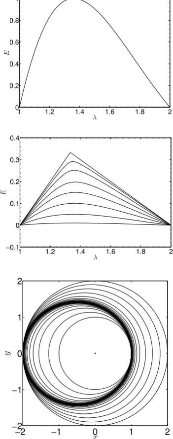
plot-ted the fundamental eccentric modeE(λ) in the top panel of Fig. 1. The amplitude is arbitrary, so this represents the shape of the disc for any amplitude according to linear the-ory. However, neighbouring orbits (for an untwisted disc) intersect if

e−λe′2

>1, (10)

which is observed to occur for this linear mode atR=Riif

A&0.143 (forRo= 2; similarly this occurs whenA&0.18

forR0= 3, and A&0.24 forR0 = 10). This suggests that

1 1.2 1.4 1.6 1.8 2 0

0.2 0.4 0.6 0.8 1

E

λ

1 1.2 1.4 1.6 1.8 2

−0.1 0 0.1 0.2 0.3 0.4

E

λ

−2 −1 0 1 2

−2 −1 0 1 2

x

y

Figure 1.Illustrative fundamental eccentric mode solutionse(λ) in a domain withRo= 2 andσ= 0 (andcs= 0.05) according to linear secular theory (top) and nonlinear secular theory (middle). The amplitude in the top panel is arbitrary. Middle: solutions with

A≈0.01,0.05,0.1,0.15,0.2,0.25,0.3 and 0.332 have been plotted. Bottom: orbital geometry in thex, y-plane for the eccentric mode withA≈0.332, showing orbits spaced equally inλ, which clearly shows the compression and near-intersection of orbits in this case.

via shocks. However, this prediction is based on linear the-ory.

Nonlinear secular theory (Eq. A10, together with the boundary conditions) predicts the shape of the eccentric mode to depend on its amplitudeA, as we illustrate in the middle panel of Fig. 1 for several amplitudes as indicated in the caption. Inspection of the functional form of the terms on the right hand side of Eq. A10 informs us why this is the case: these terms increasingly differ from those in

lin-ear theory as the orbits approach an intersection, i.e. the shape depends on the amplitude because pressure forces act to minimise intersections. This also causes the precession of the mode to differ from the predictions of linear theory, as we will demonstrate in§3.2.

With our adopted boundary conditions, nonlinear the-ory predicts a maximum attainable amplitude for the eccen-tricity, corresponding to the upper curve in the middle panel of Fig. 1, which occurs whenA≈0.332. We have plotted the orbital geometry for the eccentric disc withA≈0.332, with orbits spaced equally inλ, in the bottom panel of Fig. 8. This shows clearly the compression and near-intersection of orbits near the inner and outer boundaries for this mode, in addition to the fact that it can no longer be described purely as anm = 1 mode. The maximum value can be explained simply by considering the (untwisted) eccentric mode which is marginally intersecting, so thate−λe′ _{=±1, that also}

satisfies the boundary conditions that e(λi) = e(λo) = 0.

The solution is the piecewise linear profile

e= (_λ

λi −1, ifλ∈[λi, λm],

1−λλo, ifλ∈(λm, λo],

(11)

where

λm=

2

λ−1

i +λ−

1

o

. (12)

The maximum eccentricity of this mode is

emax≡e(λm) =

λo−λi

λi+λo

, (13)

which explains our observation of a maximum eccentricity for the fundamental eccentric mode in a domain with a given size (in numerical calculations we observeemax(λo = 2) ≈

0.332, emax(λo = 3) ≈ 0.496 and emax(λo = 5) ≈ 0.66).

This solution is what we must obtain from geometrical con-siderations simply because we force the eccentricity to van-ish at the boundaries. However, this result depends on the boundary conditions, since this limit would no longer ap-ply if e′_(λ

o) = 0, for example, and we would not obtain a

maximum eccentricity smaller than one.

3.2 Precession rates: validation of theory

According to linear theory, the eccentric mode precesses slowly in a retrograde sense due to gas pressure. To see that this must be the case, we can multiply Eq. 5 byE∗_{, seek}

solutionsE∝eiωpt _{and integrate overλto obtain:}

ωp=

c2

s

Rλo

λi λ

2_|E|2_∂

λΣ−λ3Σ|E′|2dλ

2Rλo

λi (GM λ

3₎12_Σ|E|2_dλ

, (14)

with our chosen boundary conditions (Goodchild & Ogilvie 2006). This quantity is a negative real number if∂λΣ6 0,

i.e.σ>0, indicating retrograde precession3_.

3 _{If we were to model a real system by including additional effects}

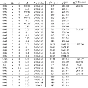
cs Ro σ A NR×Nφ Ppobs(±1) Pppred PpNS,Lin,pred 0.05 2 0 0.005 200x256 287 278.33 286.01 0.05 2 0 0.01 200x256 287 278.11

0.05 2 0 0.025 200x256 284 276.56 0.05 2 0 0.05 200x256 280 271.03 0.05 2 0 0.075 200x256 272 262.07 0.05 2 0 0.1 200x256 261 249.78 0.05 2 0 0.125 200x256 248 234.35 0.05 2 0 0.15 200x256 230 216.00

0.05 3 0 0.01 300x256 744 726.78 742.22 0.05 3 0 0.1 300x256 718 700.20

0.05 3 0 0.2 300x256 645 621.45 0.05 3 0 0.25 300x256 589 562.74 0.05 3 0 0.3 300x256 518 490.66

0.05 5 0 0.01 500x256 1629 1592.91 1627.26 0.05 5 0 0.1 500x256 1608 1571.43

0.05 5 0 0.2 500x256 1546 1509.13 0.05 5 0 0.3 500x256 1446 1402.52 0.05 5 0 0.4 500x256 1267 1231.76

0.025 2 0 0.01 200x256 1123 1112.4 1121.47 0.075 2 0 0.01 200x256 133 143.39 130.99

0.1 2 0 0.01 200x256 77 69.53 76.44 0.05 2 1.5 0.01 200x256 277 271.05 279.46 0.05 2 3 0.01 200x256 257 251.87 260.58 0.05 2 5 0.01 200x256 224 215.68 224.52 0.05 2 0 0.05 800x1024 280 271.03

0.05 2 0 0.05 400x512 280 271.03 0.05 2 0 0.05 100x128 280 271.03 0.05 2 0 0.05 50x64 287 271.03

Table 1.Table of simulations used to validate nonlinear secular theory. In each case the precession is retrograde. The error bars for

Pobs

p correspond with the time interval between output files used for this analysis.Pppredis the prediction from nonlinear secular theory (Eq. A10) and PpNS,Lin,pred is the (non-secular) prediction from solution of the two-dimensional linearised isothermal hydrodynamic equations in Appendix B (we have entered the latter in the smallestAentry in the table for each case, but it should be remembered that these results are based on a linear calculation). Simulations were run for at least one full precession period.

The precession rate depends onσ,Ro andcs, but is

in-dependent of the amplitude of the eccentric mode in linear theory. However, we have shown that nonlinear secular the-ory predicts the structure of the eccentric mode to be modi-fied if the orbits are close to intersecting, so we might expect

ωp to depend on its amplitude also. We demonstrate that

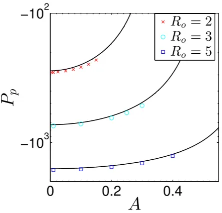
this is indeed the case in the black solid lines in Fig. 2, where we have plotted the precession period Pp= _ω2π

p against the

amplitude of the eccentric mode for several calculations with differentRo∈[2,3,5] and variousAwithσ= 0 and

assum-ing a thin disc withcs= 0.05. Gas pressure causes the mode

to precess faster, in a retrograde sense, as the eccentricity and eccentricity gradients are increased. We obtain the lin-ear prediction in the limitA→0, with a departure that is initially∝A2, before steepening for largeA. The precession period continues to shorten untilA→emax, whenPp→0,

so that the secular approximation is no longer valid. Nonlin-ear secular theory therefore predicts its own breakdown for large amplitudes, which occurs when the orbits in the disc come close to intersecting.

In Fig. 2 we have also plotted the initial precession pe-riod computed from hydrodynamical simulations (symbols according to the legend) that were run for at least one full precession period. A table of simulations used for this com-parison, and those in the rest of this section, is given in Table 1. We calculate the precession period by computing them= 1 component of the radial velocity (this quantity is

used to represent the power in bothm=±1),

ˆ

u1(R, t) =

1

π

Z 2π

0

uR(R, φ, t)e−iφdφ, (15)

from which the mean longitude of pericentre can be com-puted from

hω(t)i= 1

Ro−Ri

Z Ro

Ri

tan−1

−Im[ˆ_Re[ˆu_u1(R, t)] 1(R, t)]

dR, (16)

which is approximately valid for the eccentric mode even whenAis not small. Since this mode precesses retrogradely, hωidecreases cyclically fromπto−π, and we calculate the initial precession period by eye by checking at what time hωi ≈ π after t = 0. The data used for this analysis is output at each time unit in the simulation, giving errors of ±1 in the determination of Pobs, which we further verified

by visual inspection ofuR(R, φ, t) at these time snapshots.

Simulations with A & 0.15 for Ro = 2 were not plotted,

since the eccentric mode underwent non-negligible damping during a single precession period, as we will discuss further in§4. Fig. 2 shows that our results are in good agreement with the nonlinear secular theory for eachRo considered.

To further validate the predictions of secular theory, we have listed the observed and predicted values of Pp as

various disc (and simulation) parameters are varied in Ta-ble 1. The variation ofPpwithσandcs is reasonably

0

0.2

0.4

−10

−10

A

P

p

Ro

= 2

R

= 3

Ro

= 5

Figure 2.Precession periodPpversus peak eccentric mode am-plitudeAshowing a comparison between nonlinear secular theory (black solid lines) and the results of hydrodynamical simulations in a domainRo = 2,3 and 5 (red crosses, light blue circles and blue squares, respectively),cs = 0.05 andσ = 0. This demon-strates that the eccentric mode precesses faster as its amplitude is increased. We observe good agreement between simulations and nonlinear secular theory asAandRoare varied (with a departure of approximately 3%). Note that secular theory predicts its own breakdown for large amplitudes, asPp→0.

cs= [0.025,0.05,0.075,0.1], the fractional error

correspond-ingly takes the approximate values [1,3.2,7.5,10]%, indicat-ing a roughlyc2

s dependence for this quantity, as expected

from secular theory (Ogilvie 2001; Ogilvie & Barker 2014). To confirm that this departure indeed results from the par-tial inaccuracy of the secular approximation, we have also computed the precession frequency of anm= 1 linear eccen-tric mode by solving the two-dimensional linearised isother-mal (non-secular) hydrodynamic equations as outlined in Appendix B, for the cases listed in the table. This accu-rately matches the observed precession rates of our smallest

Asimulations in each case. For thin discs withcs.0.1, the

precession period predicted by secular theory matches the observed values to within a few percent, typically tending to predict slightly slower precession.

We have also computed the precession rate for a set of calculations with A = 0.05 as the resolution is varied, as indicated in Table 1. This indicates convergence is attained for the precession period even at low resolutions such as 100×128, but a departure appears for even lower resolutions. This suggests that simulations with typically-adopted reso-lutions would be expected to capture the precession rates of global eccentric modes, but may not accurately capture the precession of shorter wavelength modes.

3.3 Summary

We have shown that the retrograde precession of eccentric discs as a result of their gas pressure is enhanced for suf-ficiently large eccentricities and eccentricity gradients. This

dependence of the precession rate on the eccentricity and its gradient is a new result4 (though there was some numerical evidence of this in Papaloizou 2005b), and occurs because pressure forces are enhanced when the orbits come close to intersecting. While the numerical results would change if we were to adopt different boundary conditions, this gen-eral behaviour is likely to be robust since it arises from the functional form of the stress integrals (see Appendix A).

We have thoroughly validated the predictions of nonlin-ear secular theory regarding the precession rates of eccentric discs as various parameters are varied, in the regime where

ωp ≪ Ω. We find that the departure from secular theory

scales asO(c2s), typically being a few percent or smaller for

thin discs ifωp≪Ω (which we have shown to break down

at large amplitudes). We now turn to a more detailed anal-ysis of our simulation results, focussing on the long-term evolution of the eccentricity in two dimensions.

4 MORE DETAILED DISCUSSION OF SIMULATION RESULTS

4.1 Background instability: nonlinear evolution of the “Papaloizou-Pringle” instability

Our basic setup has rigid walls to confine an eccentric mode and permit a well-defined study. However, it is well known that a circular supersonic rotating shear flow in a container with one or more rigid boundaries is unstable to the de-velopment of non-axisymmetric instabilities (Papaloizou & Pringle 1984, 1985; Goldreich & Narayan 1985; Goldreich et al. 1986; Papaloizou & Pringle 1987; Kato 1987; Narayan et al. 1987). These instabilities are driven either by Kelvin-Helmholtz-type mechanisms (which require a potential vor-ticity minimum, which is not the case in our problem), or by over-reflection of spiral density waves from the corota-tion region. While most of the original work on this prob-lem focused on thick discs (referred to as “accretion tori”) where this instability excites low azimuthal wavenumber (m=O(1)) modes on a local orbital timescale, slower grow-ing instabilities with high azimuthal wavenumbers (m≫1) have also been found to occur in thin Keplerian discs (Pa-paloizou & Pringle 1987; Narayan et al. 1987; Hanawa 1987). The nonlinear evolution of these instabilities has been stud-ied by Godon (1998) (and earlier for thick “accretion tori” by Hawley 1987), where they were observed to drive sub-sonic wave activity in hydrodynamic discs.

The basic mechanism of instability in a thin nearly Ke-plerian disc can be explained as follows. An outgoing spiral density wave with frequency ωm and azimuthal

wavenum-ber m 6= 0 with a radial angular momentum flux I that approaches its corotation region (the region where the wave frequency satisfiesωm≈mΩ) is primarily reflected from its

inner Lindblad resonance (whereωm−mΩ =−κ, andκ≈Ω

is the epicyclic frequency), with the angular momentum flux in the reflected wave beingR. However, this wave is also par-tially transmitted through the corotation region (in which it is evanescent), requiring an outgoing wave to be launched

4 _{We also note that a precession rate that depends on the}

at the outer Lindblad resonance (whereωm−mΩ =κ) with

transmitted angular momentum fluxT =I − R. In a Kep-lerian disc, waves propagating inside corotation (ωm6mΩ)

carry a negative angular momentum flux (so that I < 0), whereas those outside corotation (ωm>mΩ) carry a

posi-tive flux (so thatT >0). This means thatR=I−T <I, so that the reflected wave is amplified. If there is an inner im-permeable boundary, the reflected wave will be completely reflected once more so that it will re-enter the corotation region, enabling further amplification at the expense of the Keplerian flow. This mechanism of instability, which is due to the “over-reflection” of waves from the corotation region, also occurs if there is a rigid outer boundary, but does not occur if both boundaries perfectly transmit wave energy, and it can be eliminated with sufficient viscosity.

While our primary aim is to study the evolution of ec-centric discs, this instability (which is an artifact of our model) will drive subsonic wave activity that will interact with the eccentric mode. Because of this, we briefly describe the properties of this instability for a circular disc in this section, before discussing the evolution of eccentric discs in the next. In Figs. 3 and 4, we present calculations that show the energy in the lowest ten azimuthal wavenumbers

Em(t) =

Z Ro

Ri

1

2|ˆum(R, t)|

2_{RdR, (17)}

where

ˆ

um(R, t) =

1

π

Z 2π

0

uR(R, φ, t)e−imφdφ, (18)

which is defined so that it represents the power in the so-lution with a given value of |m|, so that onlym > 0 need to be considered for this quantity. We compare three differ-ent numerical resolutions NR×Nφ: 200×256 (labelled as

L), 400×512 (labelled as M) and 800×1024 (labelled as H). Each simulation has Ro = 2,cs = 0.05, and is started

with random white noise perturbations to each component of the velocity on the grid-scale5 _{with amplitude 10}−5_c

s.

Since this instability preferentially excites high azimuthal wavenumbers and there is no explicit viscosity in our sim-ulations, we expect some dependence on resolution, though we will show that the results for M and H appear to have converged.

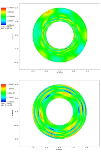
Fig. 3 illustrates that simulation L exhibits instability with the excitation ofm∼5 propagating waves byt∼2000, but this initially saturates at low amplitude. At later times,

m∼3 standing waves develop throughout the domain. We illustrate the velocity field during these stages in Fig. 5 for this simulation, in the early linear growth phase (top) and during the later phase (bottom). The RMS radial velocity driven by the instability, normalised by the sound speed,

hu/csi=

s 1

c2

sπ(R2o−R2i)

Z 2π

0 Z Ro

Ri u2

RRdRdφ, (19)

is plotted in Fig. 6 for all three simulations, along with the efficiency of angular momentum transport

α= 1

c2

sπ(R2o−R2i)

Z 2π

0 Z Ro

Ri

uR(uφ−RΩ)RdRdφ. (20)

5 _{No attempt is made to ensure that these are identical for each}

resolution adopted.

0 0.5 1 1.5 2

t

×104

10-10 10-9 10-8 10-7 10-6 10-5

m= 1 m= 2 m= 3 m= 4 m= 5 m= 6 m= 7 m= 8 m= 9 m= 10

(a) L

0 0.5 1 1.5 2

t

×104

10-10 10-8 10-6 10-4

m= 1 m= 2 m= 3 m= 4 m= 5 m= 6 m= 7 m= 8 m= 9 m= 10

(b) M

0 0.5 1 1.5 2

t

×104

10-10 10-8 10-6 10-4

m= 1 m= 2 m= 3 m= 4 m= 5 m= 6 m= 7 m= 8 m= 9 m= 10

(c) H

0 0.5 1 1.5 2

t

×104

10-10 10-8 10-6 10-4

m= 1 m= 2 m= 3 m= 4 m= 5 m= 6 m= 7 m= 8 m= 9 m= 10

(a) L,Ro= 3

0 0.5 1 1.5 2

t

×104

10-10 10-8 10-6 10-4

m= 1 m= 2 m= 3 m= 4 m= 5 m= 6 m= 7 m= 8 m= 9 m= 10

(b) M,Ro= 3

Figure 4.Same as Fig. 3, but for simulations withRo= 3 with resolutions of 300×256 (L) and 600×512 (M).

During simulation L , the maximum RMS velocities attained are very subsonic, withhui ∼10−3₋₁₀−2_c

s, and the angular

momentum transport is weak, withα.10−5_.

Simulations M and H reach larger turbulent velocities of hui ∼0.03cs and somewhat more efficient angular

momen-tum transport withα∼10−4 _{(Fig. 6) – note thatα= 10}−4

impliestvisc= R

2 i

αcsH =

1

αc2

s ≈4×10

6_{. The initial instability}

in these simulations preferentially excites m ∼ 9 compo-nents, withm∼6 dominating at later times, which differs from simulation L. However, the instability appears to be well captured with the resolution adopted for simulation M, since simulation H does not differ significantly. In addition, results do not appear to be strongly dependent on the do-main size, with simulations in a dodo-main withRo= 3 (where

resolutions L and M correspond with 300×256 and 600×512 grid-points, respectively) giving similar spectra at late times (compare Fig. 3 with Fig. 4) and broadly comparable tur-bulent velocities and angular momentum transport (Fig. 6) – note that the initial turbulent stages are different, with

m∼6 modes excited initially that remain dominant at late times. (We have also checked that the outcome of the

in-Figure 5.Radial velocity uR in the linear growth phase (top; propagating spiral waves are produced at inner boundary) and at a later stage (bottom; global radial standing waves are shown) of the instability in our lowest resolution simulation, illustrating the non-axisymmetric waves generated by the instability.

stability does not depend significantly onσ, at least where

σ61.5.)

The instability excites spiral density waves that sat-urate with subsonic velocities and lead to weak but non-negligible angular momentum transport. This instability provides background wave activity which complicates the analysis of eccentric modes in the next section. Depending on the particular waves excited by this instability, their non-linear interaction with the predominantly m= 1 eccentric mode could either drain energy from, or transfer energy into, this component. Hence, we would not expect secular theory to be valid in the presence of a strong non-axisymmetric component, given that it neglects wave-wave couplings.

Given that this instability is minimised for the resolu-tion adopted for simularesolu-tion L, we primarily focus on simu-lations using this resolution in the next section, where we turn to analyse the long-term evolution of eccentric discs.

4.2 Long-term nonlinear evolution of free eccentric modes

As in § 3.2, we initialise the flow with an eccentric mode with peak eccentricity amplitudeAand study its nonlinear evolution, focussing on its behaviour over many (50−70) precession periods.

We begin by analysing the temporal evolution of the ec-centric mode energy for variousAin Fig. 7. We plotE1 (as

dur-0 0.5 1 1.5 2

t _×104

10-3 10-2 10-1

h

u

/cs

i

L M H L,Ro=3 M,Ro=3

0 0.5 1 1.5 2

t

×104 10-7

10-6 10-5 10-4 10-3 10-2

α

L M H L,Ro=3 M,Ro=3

Figure 6. Top: RMS turbulent velocities normalised by cs (hu/csi), which are subsonic with ∼ 0.05cs. Bottom: angular momentum transportαdriven by the instability, which exhibits mean values ofα∼10−5₋₁₀−4 _{for our configuration with rigid}

boundaries.

ing the initial stages. The eccentric mode persists through-out our simulations, but experiences two different kinds of damping as the simulation progresses. Firstly, numerical dif-fusion acts to damp the eccentric mode, which is particularly pronounced for cases with higherA. Since the streamlines are then highly concentrated (see e.g. the bottom panel of Fig. 1), and there are strong eccentricity gradients, these modes experience appreciable damping by numerical diffu-sion on the grid-scale. However, this is only the most im-portant damping mechanism during the initial stages when

A&0.125. During later stages (i.e. aftert&1000), the dom-inant damping mechanism is the interaction of the m = 1 eccentric mode with other non-axisymmetric waves that are driven by the instability discussed in§4.1. These waves are excited in the absence of an eccentric mode, but interact with the eccentric mode through nonlinear interactions to generate additional non-axisymmetric components. In most cases this interaction acts to damp the eccentric mode, but it can also transfer energy into the eccentric mode in some cases e.g. seeA= 0.005 whent∼2500.

In Fig. 8, we have plotted the temporal evolution ofEm

form∈[1,10] to illustrate the growth ofm6= 1 components

0

0.5

1

1.5

2

x 10

10

10

10

10

10

10

t

E

A= 0.005

A= 0.01

A= 0.025

A= 0.05

A= 0.075

A= 0.1

A= 0.125

A= 0.15

Figure 7.Energy in the eccentric modeE1 (technically the

en-ergy in the|m|= 1 components of the flow) as a function of time for a set of simulations withRo= 2,cs= 0.05,σ= 0 for varying

A(each with a resolution of 200×256). The simulation is run for approximately 70 linear precession periods and shows that the eccentric mode persists throughout the duration of these simula-tions. It does, however, experience gradual amplitude-dependent damping.

of the solution. The top left panel repeats our results when

A= 0 (Fig. 3) to provide a point of reference. The remaining panels show the same quantity for several different values of

A. When A = 0.005, background instability occurs at ap-proximately the same time as theA= 0 case, preferentially exciting similar modes (together with those with azimuthal wavenumbers that differ by 1), and them6= 1 components of the solution saturate with similar energies (∼10−7_{). The}

m= 1 component does not undergo significant damping un-tilt∼2500, after the background instability has set in. This supports our interpretation that this damping of the eccen-tric mode is due to its interaction with non-axisymmeeccen-tric waves driven by the background instability, and not due to a separate instability of the eccentric mode itself.

In Fig. 9, we have plotted the same quantity but for a set of simulations that have double the radial and azimuthal resolution (starting with simulation M of§4.1). The eccen-tric mode evolves similarly in these cases as in the lower resolution simulations in Fig. 8. However, the background instability is excited earlier in the simulations with small

A, which leads to slightly different long-term quantitative evolution for the eccentric mode amplitude (in fact there is slightly more efficient damping in some of these simulations compared with those with the lower resolution, demonstrat-ing that the amplitude decay is not primarily due to numer-ical diffusion).

AsAis increased, this instability occurs sooner in the simulation, presumably because there is more energy in

0 0.5 1 1.5 2 t

×104

10-10 10-9 10-8 10-7 10-6 10-5

m= 1 m= 2 m= 3 m= 4 m= 5 m= 6 m= 7 m= 8 m= 9 m= 10

(a)A= 0

0 0.5 1 1.5 2

t

×104

10-10 10-9 10-8 10-7 10-6 10-5

m= 1 m= 2 m= 3 m= 4 m= 5 m= 6 m= 7 m= 8 m= 9 m= 10

(b)A= 0.005

0 0.5 1 1.5 2

t

×104

10-10

10-8

10-6

10-4

m= 1 m= 2 m= 3 m= 4 m= 5 m= 6 m= 7 m= 8 m= 9 m= 10

(c)A= 0.01

0 0.5 1 1.5 2

t

×104

10-10

10-8

10-6

10-4

m= 1 m= 2 m= 3 m= 4 m= 5 m= 6 m= 7 m= 8 m= 9 m= 10

(d)A= 0.05

0 0.5 1 1.5 2

t

×104

10-10

10-8

10-6

10-4

10-2

m= 1 m= 2 m= 3 m= 4 m= 5 m= 6 m= 7 m= 8 m= 9 m= 10

(e)A= 0.1

0 0.5 1 1.5 2

t

×104

10-10

10-8

10-6

10-4

10-2

m= 1 m= 2 m= 3 m= 4 m= 5 m= 6 m= 7 m= 8 m= 9 m= 10

(f)A= 0.15

Figure 8.Energy in different azimuthal wavenumber components of the solution (Em) for m ∈ [1,10] as a function of time for several different amplitudesAfor a set of simulations with 200×

256 grid points. The instability that occurs in the absence of an eccentric mode also occurs whenA6= 0, which excites non-axisymmetric waves that subsequently interact with the eccentric mode, generally leading to damping. However, the eccentric mode itself does not appear to be subject to separate instabilities in two dimensions.

other non-axisymmetric components typically saturate with similar power to theA = 0 case. In all simulations, there is an amplitude- and time-dependent damping (or transient growth, as briefly observed at t ≈ 2000 in the A = 0.005 simulation in Fig. 8) of the eccentric mode due to its in-teraction with waves driven by the background instability. However, our interpretation, which is guided by Figs. 8 and 9, is that the eccentric mode does not appear to be subject to additional instabilities due to the presence of a nonzero eccentricity (at least in two dimensions), only to the finite-A

modification of the instability that occurs when A= 0 due to our adoption of rigid walls.

In Fig. 10, we plot|uˆ1(R)| att= 0 (solid black lines)

and t= 20000 (red dashed lines; marking the end of each

0 0.5 1 1.5 2

t

×104

10-10

10-8

10-6

10-4

m= 1 m= 2 m= 3 m= 4 m= 5 m= 6 m= 7 m= 8 m= 9 m= 10

(a)A= 0

0 0.5 1 1.5 2

t

×104

10-10

10-8

10-6

10-4

m= 1 m= 2 m= 3 m= 4 m= 5 m= 6 m= 7 m= 8 m= 9 m= 10

(b)A= 0.01

0 0.5 1 1.5 2

t

×104

10-10

10-8

10-6

10-4

m= 1 m= 2 m= 3 m= 4 m= 5 m= 6 m= 7 m= 8 m= 9 m= 10

(c)A= 0.05

0 0.5 1 1.5 2

t

×104

10-10

10-8

10-6

10-4

10-2

m= 1 m= 2 m= 3 m= 4 m= 5 m= 6 m= 7 m= 8 m= 9 m= 10

(d)A= 0.1

Figure 9.Same as Fig. 8 except for a set of simulations with 400×512 grid points.

1 1.5 2

0 0.002 0.004 0.006 0.008 0.01 ˆ u1 R

t= 0

t= 20000

(a)A= 0.01

1 1.5 2

0 0.01 0.02 0.03 0.04 0.05 ˆ u1 R

t= 0

t= 20000

(b)A= 0.05

1 1.5 2

0 0.02 0.04 0.06 0.08 0.1 ˆ u1 R

t= 0

t= 20000

(c)A= 0.1

1 1.5 2

0 0.05 0.1 ˆ u1 R

t= 0

t= 20000

(d)A= 0.15

Figure 10.Magnitude of the radial velocity in them= 1 com-ponent of the solution (|uˆ1|) as a function ofRat the beginning

1 1.5 2 −3

−2 −1 0 1 2 3

ω

R

(a)A= 0.01

1 1.5 2

−3 −2 −1 0 1 2 3

ω

R

(b)A= 0.1

Figure 11.Longitude of pericentreωas a function ofRfor simu-lations at timest= [0,30,60,90,120,150,180,210,230,260,290]. This illustrates that the eccentric disc remains approximately un-twisted during one precession period, though slight twists can develop.

simulation), which shows the damping of the eccentric mode. In addition, this demonstrates that the eccentric mode re-mains coherent, persisting throughout the duration of these simulations in a form that is similar to the initial conditions. The similarity in the mode shape at these two times sup-ports the validity of secular theory in describing the shapes of these modes.

Our initial disc model is untwisted, but we do not con-strain it to remain so. In Fig. 11, we showω(R) forA= 0.01 and A= 0.1, for times t∈[0,300] (slightly more thanPp)

spaced in intervals of 30 time units. At t = 0, the disc is untwisted with ω = π, but slight twists develop dur-ing the course of the simulation, preferentially near to the outer boundary. However, the disc remains approximately untwisted as it evolves throughout these simulations with a net twist that is small even whenA = 0.1 (smaller than 0.5 rads). It is possible that numerical damping, which is likely to act in a similar way to a shear viscosity (Ogilvie 2001), could be responsible for this twist in the outer re-gions (where the grid cells are largest), thereby preventing the disc from remaining entirely untwisted (also, if the ini-tial conditions are not exact nonlinear solutions, some twist would be expected to develop). Alternatively, since e →0 as R → 2, the phase of the complex eccentricity becomes undefined at this location, so we might expect the twist at this location to be arbitrary.

Finally, we analyse the decay rate of the eccentric mode, which we plot in Fig. 12 for several simulations, showing the effects of varying the resolution. This picture is not clear-cut because the background instability is stronger for the higher resolution case. This illustrates that eccentric modes in two dimensions persist for a very long time, even in the presence of amplitude-dependent wave-wave interactions and numer-ical damping.

4.3 Summary

In this section we have presented the results of nonlinear hydrodynamical simulations designed to study the long-term evolution of eccentric discs in two dimensions. Eccen-tric discs remain coherent and do not appear to be sub-ject to instabilities as a result of their free eccentricity in

0 0.05 0.1 0.15

−2 −1.5 −1 −0.5 0 0.5

1x 10 −4

A ˙_E/E

max200 mean200 max400 mean400

Figure 12. Decay rate of maximum and mean eccentricity in the eccentric mode ˙E/E, as a function of A at resolutions of 200×256 and 400×512. The error bars represent the maximum and minimum damping rates observed in these simulations. The red lines are plotted for reference, and have approximate slopes of −2×10−4 _{and −5×10}−4_{, respectively. Note that ˙E/E ≈}

−5×10−5 _{corresponds with a damping time of approximately}

2×104_.

two dimensions, and would presumably persist forever if there was no background instability. They are, however, damped (typically) by their nonlinear interaction with non-axisymmetric spiral density waves – these waves are driven by a background (“Papaloizou-Pringle”) instability in our setup with rigid walls6_{. In real discs there are various}

mech-anisms that could produce such an incoherent ensemble of non-axisymmetric waves e.g. additional sources of turbu-lence such as magneto-rotational instability (e.g. Heinemann & Papaloizou 2009a,b), gravitational instability (e.g. Pa-paloizou & Savonije 1991; Laughlin & Rozyczka 1996), con-vection (e.g. Mamatsashvili & Rice 2011), or possibly the tidal interaction between multiple proto-planets and the disc.

Previous simulations of eccentric modes by Papaloizou (2005b) used linear secular theory to construct the initial conditions. This enhances the damping of the eccentric mode due to the generation of shocks at the inner boundary of the domain, since we have observed the linear mode to cause orbital intersections ifA is sufficiently large. On the other hand, the modes that we have input using nonlinear sec-ular theory do not experience such strong shock-induced damping, as indicated in Fig. 7. These modes do experi-ence amplitude-dependent damping by numerical diffusion, which can be particularly strong for largeA cases, where the orbits are closer to intersecting. But in our simulations the most important damping mechanism is the interaction of the eccentric mode with other non-axisymmetric waves.

6 _{This instability also occurs (with a similar growth rate) with}

5 CONCLUSIONS

In this paper we have studied fundamental aspects of eccen-tric gas discs that should have general applicability. We have derived analytically a nonlinear secular theory for isothermal two-dimensional untwisted eccentric Keplerian discs (valid for arbitrary eccentricities and eccentricity gradients for which neighbouring orbits do not intersect; Appendix A), and verified its predictions with idealised hydrodynamical simulations using the PLUTO code. Linear secular theory is found to accurately describe the structures and precession rates of eccentric discs with small eccentricities (and eccen-tricity gradients), which precess in a retrograde sense due to gas pressure. Discs with larger eccentricities (and eccentric-ity gradients) are observed to precess at a faster rate, which we have explained as a modification of the pressure forces, and resulting disc structure to prevent orbital intersections, that occurs when the orbits in a disc nearly intersect.

The nonlinear modification of the pressure forces might be particularly important for the highly eccentric discs pro-duced in tidal disruption events (Guillochon et al. 2011; Liu et al. 2013; Guillochon et al. 2014; Coughlin & Nixon 2015), or for narrow eccentric gas rings (cf. Borderies et al. 1983, which was applied to planetary rings). Another potential application is to the period excess in superhump binary sys-tems, which is thought to be explained due to the precession of an eccentric gaseous disc (Whitehurst 1988; Lubow 1991; Murray 2000; Goodchild & Ogilvie 2006; Smith et al. 2007). However, there is observational evidence of temporal vari-ability of the period excess (Mason et al. 2008; Nakata et al. 2014), which may in part be caused by evolution of the pres-sure forces due to the varying eccentricity and eccentricity gradients in the disc. It would be worthwhile to apply nonlin-ear secular theory to this problem (e.g. extending Goodchild & Ogilvie 2006) in order to explore this possibility further.

Eccentric discs do not appear to exhibit hydrodynamic instability as a result of their free eccentricity in two di-mensions, and we would expect them to essentially persist forever in our simulations except for their interaction with non-axisymmetric spiral density waves excited by a back-ground (Papaloizou-Pringle) instability (which arises in our setup with rigid walls), in addition to numerical viscosity. Presumably the eccentricity would be damped on the disc (turbulent) viscous timescale, but our simulations are not run for this duration (the viscous timescale is very long be-cause the background instability transports angular momen-tum only weakly). Eccentricity can also be affected by non-adiabatic thermal processes, not considered in this paper. Indeed, (Statler 2001) has argued that a uniform eccentric-ity is preferred because the surface denseccentric-ity of the disc is then constant around each orbit. However, even in this case the fluid undergoes periodic compression because of the varia-tion of vertical gravity around the elliptical orbit (which is not captured in two dimensions).

Our observation that gas discs with free eccentricities can remain eccentric for thousands of orbital periods (Fig. 7) is potentially important regarding the interpretation of ob-served large-scale asymmetries in gas discs. In particular, the presence of such asymmetries is often used to infer the presence of perturbing planets (e.g. Reg´aly et al. 2014; Hashimoto et al. 2015; Pinilla et al. 2015). However, since we have shown that eccentric modes can be long-lived features,

there are alternative mechanisms in addition to perturbing planets that can induce free eccentricity, e.g. gravitational instabilities in the gas disc during the pre-main sequence phase (Adams et al. 1989).

However, it should be noted that any conclusions re-garding the longevity of disc eccentricities are based on two-dimensional simulations with only a weak background in-stability. In three dimensions eccentric discs are subject to a parametric instability that excites small-scale inertial waves (Papaloizou 2005a; Barker & Ogilvie 2014). This is expected to lead to enhanced damping of the disc eccentricity and ec-centricity gradients (Papaloizou 2005b), but further work adopting a realistic vertical disc structure is required to de-termine its nonlinear outcome. The simulations presented in this paper provide a starting point to allow us to undertake such calculations.

ACKNOWLEDGEMENTS

AJB is supported by the Leverhulme Trust and Isaac New-ton Trust through the award of an Early Career Fellow-ship. The early stages of this research were supported by STFC through grants ST/J001570/1 and ST/L000636/1. We would like to thank the referee for constructive com-ments that led us to strengthen our conclusions.

APPENDIX A: NONLINEAR SECULAR THEORY OF ECCENTRIC DISCS

In this section we derive analytically a nonlinear secular the-ory for eccentric discs in two dimensions utilising the local model of Ogilvie & Barker (2014), for the case of an un-twisted isothermal disc in which λω′ _{= 0, i.e. the orbits}

are aligned (for which nonlinear pressure effects are likely to be minimised). While the formalism can be extended to the case of a twisted disc including viscosity, and to discs with different thermodynamic behaviour (Ogilvie 2001), we do not believe it to be possible to derive the corresponding nonlinear theory analytically in terms of algebraic functions (particularly the stress integrals) except for this special case. We denote cosθbycand sinθbysto simplify the expres-sions below, where theθ =φ−ω(λ), is the true anomaly. At eachλ, the reference orbit is Keplerian, so

R=λ(1 +ec)−1_{, (A1)}

and the angular velocity of the orbital motion is

Ω = r

GM

λ3 (1 +ec)

2_{. (A2)}

The orbital period for a fluid element with this orbit is

P= Z 2π

0

Ω−1_{dθ= 2π} r

λ3

GM(1−e

2₎−32, (A3)

and its specific angular momentum isℓ=√GM λ.

eccentric disc with non-intersecting orbits:

Z Z

JR2Tλφdφdz = 0, (A4)

Z Z

JR2Tλφeiφdφdz = ic

2

se e2−1

λM (λe′₎2 e

2

−eλe′₋₁

+p(e2_{−1) ((e−λe}′₎2₋₁₎ !

,

(A5)

Z Z

JRλTλλeiφdφdz =

c2

s 1−e2

3/2 M (λe′₎2

e+λe′_−e3 √

1−e2

− e+λe

′_+e2_λe′_−e3

q

1−(e−λe′₎2

!

, (A6)

Z Z

JR2Tφφeiφdφdz = c2seM, (A7)

whereTij_=−pgij_andJ=RR

λ. In each case the integrals

are over the full extent of the disc in φ and z. We have defined Rλ ≡ ∂λR and Rφ ≡ ∂φR, so that the relevant

components of the metric tensor are

gλλ=R

2_+R2

φ

R2_R2

λ

, gλφ=−_RR2_Rφ

λ

, gφφ= 1

R2. (A8)

The one-dimensional mass density is

M=

Z Z

JΣ dφ. (A9)

The mass and angular momentum do not evolve since the first integral above vanishes, which results from us ne-glecting shear viscosity. The complex eccentricity evolves ac-cording to

ℓM∂tE =

Z Z

2eiφ∂λ(JR2Tλφ)−iλeiφ∂λ(JRλTλλ)

−i eiφJR2Tφφ−JR 2

λ e

iφ_Tλφ_dφdz,(A10)

which is a type of nonlinear Schr¨odinger differential equation (that is second order inλ).

For general initial conditions, the time-evolution will produce a twist in the disc, but it is possible to seek modal solutions that remain untwisted. In this case, inputting the stress integrals above leads to an equation for the evolution of the complex eccentricity for any eccentricity and eccen-tricity gradient for an untwisted disc, as long as the orbits do not intersect. The final form of this equation after sub-stituting the stress integrals is too complicated to be worth writing down in closed form here. It can, however, be com-puted in Mathematica and exported to text format for input in our Matlab scripts that are used to solve Eq. A10.

We seek modesE∝eiωpt_{that precess slowly at the rate} ωp, so that Eq. A10 is converted to an eigenvalue problem

of the form

ωpe=f(λ, e, e′, e′′), (A11)

subject to appropriate boundary conditions, wheref is in general a nonlinear function of its arguments.

The behaviour of the stress integrals for large e,e′ _is

straightforward to understand. As the orbits become closer to intersecting ((e−λe′₎2

→ 1) or e → 1 or (λe′₎2 → 1, strong pressure forces arise, which modify the eccentricity

profile so that the orbits do not intersect. An interesting result of these forces is that they modify the global preces-sion rate of the mode throughout the disc so that it pre-cesses more rapidly in a retrograde sense as the orbits be-come closer to intersecting, even if this near intersection only occurs in a small region of the disc. We note that the for-malism of Borderies et al. (1983) for narrow eccentric rings (with small eccentricities but arbitrary eccentricity gradi-ents) applied to an isothermal gas also predicts a precession rate (their Eq.13) that depends on the eccentricity gradient, and which diverges in the limit of intersecting orbits. This is consistent with our results.

The 2D isothermal model is a simplification of a real-istic 3D eccentric disc. The isothermal case (with adiabatic index of 1) is the most compressible 2D model that we can consider, where the pressure increase for a given stream-line convergence is minimised (over less compressible mod-els with adiabatic indices larger than 1). However, in 3D the disc can also expand vertically, which may somewhat allevi-ate this pressure increase. However the qualitative behaviour of the 2D isothermal model is likely to carry over to more realistic models.

APPENDIX B: LINEAR NON-SECULAR THEORY IN 2D

As listed in Table 1, we solve the eigenvalue problem for the full (non-secular) isothermal hydrodynamical equations in two dimensions to compute the precession frequency of the fundamentalm= 1 linear eccentric mode, to allow compar-ison with simulations and secular theory. We assume linear perturbationsu′

R, u′φ,Σ′∝ei(φ−ωpt), which satisfy

−iˆωu′

R= 2Ωu′φ−

c2s

Σb

∂RΣ′+c

2

sΣ′

Σ2

b

∂RΣb, (B1)

−iˆωu′

φ=−(2Ω +R∂RΩ)u′R−

ic2s

RΣ

′_{, (B2)}

−iˆωΣ′_=−Σ

b

_u′

R

R +∂Ru

′

R

−u′

R∂RΣb−

iΣb

R u

′

φ,(B3)

where ˆω=ωp−Ω, subject to the BCs thatu′R= 0 atR=Ri

andR=Ro. In this case

Ω = Ω0R−

3 2

1−σc

2

s

Ω2 0

R

1 2

, (B4)

where we have taken into account the radial pressure gra-dient in full. This is solved using a Chebyshev collocation method (adopting 101 points in radius, which we find to be more than sufficient to compute the fundamental mode), which converts the problem to a standard eigenvalue prob-lem that can be solved (for which we use a QZ method) to compute the precession frequencyωp.

REFERENCES

Adams F. C., Ruden S. P., Shu F. H., 1989, ApJ, 347, 959 Barker A. J., Ogilvie G. I., 2014, MNRAS, 445, 2637 Bitsch B., Crida A., Libert A.-S., Lega E., 2013, A&A, 555,

A124

Chiang E. I., Goldreich P., 2000, ApJ, 540, 1084 Coughlin E. R., Nixon C., 2015, ApJL, 808, L11

D’Angelo G., Lubow S. H., Bate M. R., 2006, ApJ, 652, 1698

Godon P., 1998, ApJ, 502, 382

Goldreich P., Goodman J., Narayan R., 1986, MNRAS, 221, 339

Goldreich P., Lynden-Bell D., 1965, MNRAS, 130, 125 Goldreich P., Narayan R., 1985, MNRAS, 213, 7P Goldreich P., Sari R., 2003, ApJ, 585, 1024 Goodchild S., Ogilvie G., 2006, MNRAS, 368, 1123 Guillochon J., Loeb A., MacLeod M., Ramirez-Ruiz E.,

2014, ApJL, 786, L12

Guillochon J., Manukian H., Ramirez-Ruiz E., 2014, ApJ, 783, 23

Guillochon J., Ramirez-Ruiz E., Lin D., 2011, ApJ, 732, 74 Hanawa T., 1987, A&A, 185, 160

Hashimoto J., et al., 2015, ApJ, 799, 43 Hawley J. F., 1987, MNRAS, 225, 677

Hawley J. F., Gammie C. F., Balbus S. A., 1995, ApJ, 440, 742

Heinemann T., Papaloizou J. C. B., 2009a, MNRAS, 397, 52

Heinemann T., Papaloizou J. C. B., 2009b, MNRAS, 397, 64

Kato S., 1987, PASJ, 39, 645

Kley W., Dirksen G., 2006, A&A, 447, 369 Laughlin G., Rozyczka M., 1996, ApJ, 456, 279 Lee E., Goodman J., 1999, MNRAS, 308, 984

Liu S.-F., Guillochon J., Lin D. N. C., Ramirez-Ruiz E., 2013, ApJ, 762, 37

Lubow S. H., 1991, ApJ, 381, 259

Mamatsashvili G. R., Rice W. K. M., 2011, MNRAS, 417, 634

Mason P. A., Robinson E. L., Gray C. L., Hynes R. I., 2008, ApJ, 685, 428

Mignone A., Bodo G., Massaglia S., Matsakos T., Tesileanu O., Zanni C., Ferrari A., 2007, ApJS, 170, 228

Murray C. D., Dermott S. F., 1999, Solar system dynamics Murray J. R., 2000, MNRAS, 314, L1

Nakata C., Kato T., Nogami D., Pavlenko E. P., Ohshima T., de Miguel E., Stein W., Siokawa K., Morelle E., Itoh H., Dubovsky P. A., Kudzej I., Maehara H., Henden A., Goff W. N., Dvorak S., Antonyuk O. I., Muyllaert E., 2014, PASJ, 66, 116

Narayan R., Goldreich P., Goodman J., 1987, MNRAS, 228, 1

Ogilvie G. I., 2001, MNRAS, 325, 231 Ogilvie G. I., 2008, MNRAS, 388, 1372

Ogilvie G. I., Barker A. J., 2014, MNRAS, 445, 2621 Okazaki A. T., 1991, PASJ, 43, 75

Papaloizou J. C., Savonije G. J., 1991, MNRAS, 248, 353 Papaloizou J. C. B., 2002, A&A, 388, 615

Papaloizou J. C. B., 2005a, A&A, 432, 743 Papaloizou J. C. B., 2005b, A&A, 432, 757

Papaloizou J. C. B., Nelson R. P., Masset F., 2001, A&A, 366, 263

Papaloizou J. C. B., Pringle J. E., 1984, MNRAS, 208, 721 Papaloizou J. C. B., Pringle J. E., 1985, MNRAS, 213, 799 Papaloizou J. C. B., Pringle J. E., 1987, MNRAS, 225, 267 Papaloizou J. C. B., Savonije G. J., Henrichs H. F., 1992,

A&A, 265, L45

Pfuhl O., Gillessen S., Eisenhauer F., Genzel R., Plewa P. M., Ott T., Ballone A., Schartmann M., Burkert A., Fritz T. K., Sari R., Steinberg E., Madigan A.-M., 2015, ApJ, 798, 111

Pinilla P., de Juan Ovelar M., Ataiee S., Benisty M., Birn-stiel T., van Dishoeck E. F., Min M., 2015, A& A, 573, A9

Press W. H., Teukolsky S. A., Vetterling W. T., Flan-nery B. P., 1992, Numerical recipes in FORTRAN. The art of scientific computing. Cambridge: University Press, —c1992, 2nd ed.

Reg´aly Z., Kir´aly S., Kiss L. L., 2014, ApJL, 785, L31 Saini T. D., Gulati M., Sridhar S., 2009, MNRAS, 400,

2090

Smith A. J., Haswell C. A., Murray J. R., Truss M. R., Foulkes S. B., 2007, MNRAS, 378, 785