Aspects of the Nutrition and Physiology
of
Eucalyptus glob ulus
by
Andrew Edward Knowles, BSc (Hons)
Submitted in fulfilment of the requirements for the Degree of
Doctor of Philosophy
This thesis contains no material which has been accepted for a degree or diploma by the University or any other institution, except by way of background information and duly acknowledged in the thesis.
To the best of my knowledge and belief this thesis contains no material previously published or written by another person except where due
acknowledgement is made in the text of the thesis, nor does the thesis contain any material that infringes copyright.
Statement of Authority
This thesis may be made available for loan and limited copying in accordance with the Copyright Act 1968.
Abstract
Nutrient deficiency in forests is an international concern. In Europe and north-eastern North America, new forms of forest "die-back" are being associated with soil magnesium, potassium and calcium deficiencies, often in conjunction with acid soils. In South Africa, the soils are often extremely infertile, lacking in most of the macronutrients. New Zealand, a country with extensive forestry estates, has soil that is abundant in both potassium and magnesium, yet the magnesium is in a form that is unavailable to plants. And in Australia the age of the soil and the relatively intensive cropping of the existing plantations have led to concerns about their current and future health.
While fertilization can ameliorate nutrient deficiency, such fertilisation can itself lead to reduced productivity through increased leaching of other cations freed from the soil matrix by the application. Even without fertilization, poor "balance" between the nutrients present in the soil is believed to decrease yield. Early identification of sub-optimal nutrition can reduce the economic effects of poor growth in plantations. There are many indicators used for inferring sub-optimal nutrition, but all require a degree of calibration which, itself, requires knowledge of the plants' nutritional requirements.
To investigate the base cation requirements of the common plantation forestry species Eucalyptus globulus, three two-factor hydroponic experiments were performed. Potassium, magnesium and calcium were supplied at three different concentrations, which were chosen such that the range of concentrations was around that found in Australian forestry plantations. Furthermore, the chosen concentrations allowed observation of the effects of a wide range of base cation ratios.
mass) was related to the concentrations of supplied potassium and magnesium: the lowest concentrations (10 [tM) were clearly sub-optimal with the growth significantly depressed in comparison with the other two treatments (500 11M and 5,000 iM), which were not significantly different from each other. On the other hand, the plants were indifferent to the supplied concentration of calcium,
displaying neither depressed growth or symptoms that could be attributable to insufficient or excessive calcium, despite the wide range of concentrations supplied (10 !AM to 5,000 uM). It was evident from the chlorophyll content and the fluorescence parameters that the photosynthetic apparatus of the plants was not under stress, nor were there any significant differences between treatments, in contrast to the highly significant effects of treatments on plant biomass and foliar concentration.
The uptake of the base cations potassium, magnesium and calcium was very closely related, although not linearly, to the concentrations of those cations
available in the growth medium, and there was excellent correspondence between shoot and root cation concentrations. The correspondence between individual shoot cation concentrations and plant dry weight was, however, less than satisfactory.
Interactions between base cations in the growth medium are often blamed for inadequate nutrition leading to poor growth, but interactions between potassium, magnesium and calcium within the roots and shoots of the experimental plants were not evident. Cation ratios are commonly used in plant nutrition experiments to provide an insight into the "balance" between pairs of nutrients. Investigation of ratios in the current experiment indicated that the ratios provided no
information that could not be gained from considering the individual ions.
Pinus radiata is Australia's most commonly grown plantation softwood. Unlike Eucalyptus species, Pinus radiata is known to exhibit potassium and magnesium deficiency symptoms. Moreover, anecdotal evidence suggests that Pinus radiata has greater requirement for base cations than does Eucalyptus globulus.
biological indicator of the nutritional status of Eucalyptus plantations. To this end, Pinus radiata were grown under similar conditions as the previously studied Eucalyptus globulus.
It was found that the potassium and magnesium requirements of the two species were very different, with Pinus radiata requiring significantly more potassium, but significantly less magnesium, than Eucalyptus globulus. The eucalypts' critical concentrations (concentrations giving 90% of the maximal growth) were found to be 1801.tM for potassium and 12611M for magnesium, while the pine's critical concentrations were 220 j.tM for potassium (but at 80% maximal growth), and 63 i.iM for magnesium. It follows that Pinus radiata would not be useful as a bioassay for Eucalyptus globulus.
Using nutrient concentrations in gross plant organs can lead to errors in
interpretations as they are, effectively, the net sum of all cellular fluxes since the germination of the seed. Rates of uptake, therefore, can be only crudely
ascertained and interactions between nutrients can only be inferred. Using radio-isotopes shortens the integration period, but is still a "bottom line" picture. Ultimately, nutrient uptake occurs at a cellular level, and is measurable as an ion flux using potentiometric ion-selective electrodes. In response to changing local conditions, ion fluxes can vary in magnitude and direction on a time scale of minutes; with simultaneous measurement of two or more ions it is possible to assess ion flux stoichiometry (whence interactions) and investigate molecular mechanisms behind ion fluxes.
It has been found that ion-selective electrode membranes may react to more than one ion, confounding observations. For example, two common physiological ion pairs interfere: magnesium liquid ion exchangers respond to calcium, and sodium to potassium, which causes problems. The magnitude and non-linear nature of the response renders difficult the "disentanglement" of the fluxes. A mathematical solution to this problem was proposed in the 1950s which, while closely
To allow measurement of flux responses in more natural conditions, an empirical equation was developed to allow the separation of magnesium-calcium and sodium-potassium fluxes. This permitted the first published, real-time measurements of magnesium fluxes around plant roots.
Simultaneous measurement of potassium, magnesium and calcium fluxes around the roots of Eucalyptus globulus and Triticum aestivum were performed under varying conditions in an attempt to ascertain the mechanisms of uptake and
whether there was competition between ions at the root surface, which is the most obvious location for ionic interaction. Analysis of the flux records indicated that the fluxes of the monovalent potassium was not affected by, nor had any effect on, the divalent cations, from which it could be concluded that the passive fluxes resulting from the applied stimuli were facilitated by channels that were selective between monovalent and divalent ions.
Oscillatory net ion fluxes from roots have previously been observed in the cations potassium, calcium, and hydrogen in the rapidly growing parts of a range of crop species, but whether such oscillations are present in mature, non-growing parts of plants or in tree species, was unknown. Observations confirmed that oscillatory cation fluxes could be found in the mature regions of plant roots, and were
characteristic for Eucalyptus globulus. In addition, oscillations were observed in magnesium fluxes, the first published reports of such phenomena. Further, simultaneous measurement of spatially-separated proton fluxes indicated that, while the period of the oscillations were similar, there were phase-differences between locations.
Acknowledgements
The following people have provided invaluable assistance to me during the course of this project, and many thanks are due to them.
From the School of Agricultural Science, University of Tasmania: Dr Sergey Shabala
Dr Philip Brown Mr Bill Peterson Ms Angela Richardson
From the CRC for Sustainable Production Forestry: Dr Philip Smethurst
Dr Chris Beadle Mr Keith Churchill Ms Anne Wilkinson Mrs Judy Sprent
From the School of Physics, University of Tasmania: Dr Ian Newman
Thanks must also go to Professor Barbara Hawkins and Professor Benoit Cote, the markers of this thesis. Their careful reading and helpful suggestions were greatly appreciated.
Tab
le
of
Con
ten
ts
Abstract 4
Acknowledgements 8
Table of Contents 9
Table of Figures 11
Table of Tables 15
1
.In
troduc
t
ion
19
2
.Effec
ts
of
Base
Ca
t
ion
Concen
tra
t
ions
and
Ra
t
ios
on
the
Dry
We
igh
t
,
Nu
tr
ien
t
Concen
tra
t
ions
and
Ra
t
ios
,
and
F
luorescence
Parame
ters
of
Euca
lyp
tus
g
lobu
lus
seed
l
ings
.
26
2.1. Introduction 26
2.2 Materials and Methods 29
2.3. Results 39
2.4. Discussion 57
2.5. Conclusions 75
Appendix 2.A. Differences Between Treatmentsinthe Two-factor
Concentration Experiments 78 Appendix 2.B. Some Leaf Chlorophyll Fluorescence Theory 91 Appendix 2.C. Eucalyptus Leaf Base Cation Concentrations 94 Appendix 2.D. Further Details of Nutrient Treatments ... 94
3
.Compar
ison
of
the
Base
Ca
t
ion
Requ
iremen
ts
of
Euca
lyp
tus
g
lobu
lus
and
P
inus
rad
ia
ta
seed
l
ings
.
98
3.1. General Introduction 98 3.2. Materials and Methods 993.3. Results 101
3.4. Discussion 108
3.5. Conclusions 114
Appendix 3.A. Pinus radiata Organ Base Cation Concentrations 116
4
.Overcom
ing
the
Prob
lem
of
Non-
idea
l
L
iqu
id
Ion
Exchanger
Se
lec
t
iv
i
ty
in
M
icroe
lec
trode
Ion
F
lux
Measuremen
ts
117
4.1. Introduction 117
4.5 Conclusion 135
5
.Roo
t
Ce
l
l
Transmembrane
Transpor
t
137
5.1. Introduction 137
5.2. Ion Transportin Plant Roots 137 5.3. Passive Transportersinthe Root Cell Plasma Membrane 140 5.4. Active Transportersinthe Root Cell Plasma Membrane 145
5.5. Conclusion 152
6
.Base
Ca
t
ion
F
luxes
Around
the
Roo
ts
of
Euca
lyp
tus
g
lobu
lus
seed
l
ings
153
6.1 Introduction 153
6.2 Materials and Methods 154
6.3. Results 159
6.4. Discussion 174
6.5. Conclusions 183
7
.Osc
i
l
la
tory
Ca
t
ion
F
luxes
around
the
Roo
ts
of
Euca
lyp
tus
g
lobu
lus
and
Tr
i
t
icum
aes
t
ivum
Seed
l
ings
.
184
7.1 Introduction 184
7.2 Materials and Methods 186
7.3. Results 188
7.4. Discussion 192
7.5. Conclusions 197
8
.Genera
l
Conc
lus
ions
198
Table of Figures
Figure 2.1. Variation in plant dry weight with supplied (a) magnesium and calcium; (b) potassium and magnesium; and (c) potassium and calcium Error bars are the s.e.m. Points within graphs that are labelled with identical letters are not significantly different from each other.
44
Figure 2.2. Variation in plant dry weight with supplied (a) potassium and (b) magnesium. The solid lines represent the regressions given in section 2.3.1; in the case of (b) the points at 40 uM were not included. 45 Figure 2.3. Treatment effect on normalised dry weight. The dry weights in the individual experiments were normalised against their respective MMM treatment, and combined where appropriate. This gives an indication of the effects of the treatments relative to each other. Error bars are give the 99% range based upon the s.e.m. Treatment codes are read as K above Mg above Ca.
45
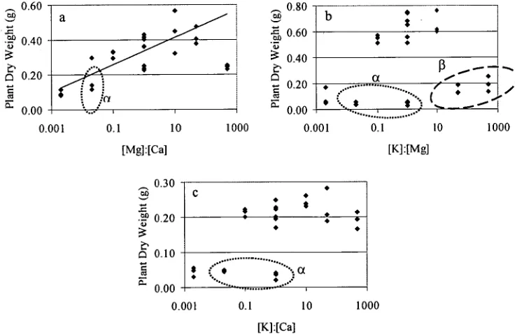
Figure 2.4. Effect of base cation ratios on ratio on average plant dry weight: (a) Mg:Ca, (b) K:Mg, (c) K:Ca. The solid line in (a) represents the regression of the plant dry weight on the natural logarithm of the ratio. Groups of points marked a and 13 are from low potassium and low magnesium treatments, respectively.
46
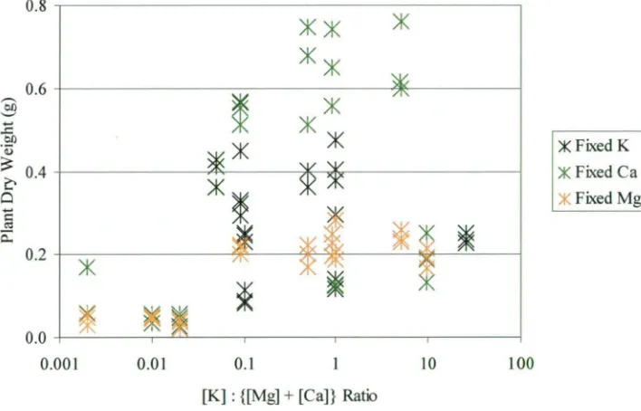
Figure 2.5. Effect of monovalent:divalent cation ratio on ratio on plant dry weight. The different colours relate to different experiments: * — fixed
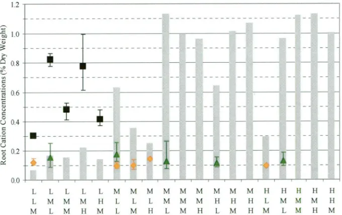
potassium; * — fixed magnesium; * — fixed calcium. 47 Figure 2.6. Variation of root cation concentrations at the lowest supplied
concentrations of those nutrients. Key: • ; • magnesium; • calcium. The error bars represent the lowest and highest concentrations for that cation and treatment. Treatment codes are read as K above Mg above Ca. The grey bars are the normalised biomass values from figure 2.3 included for reference: the values on the y-axis apply directly.
48
Figure 2.7. Variation of root base cation concentrations with supplied base cations: (a) potassium; (b) magnesium; (c) calcium. The different colours relate to different experiments: * — fixed potassium; * — fixed magnesium; * — fixed calcium. The solid lines are the regressions the equations for which are in table 2.7.
49
Figure 2.8. Relationships between Eucalyptus globulus root nutrient
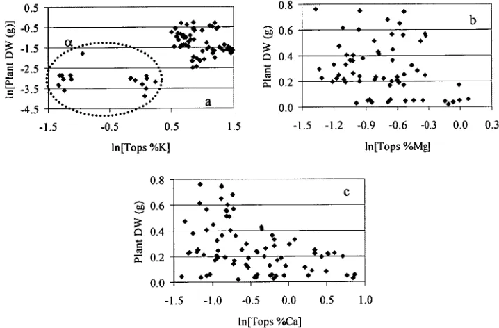
concentrations: (a) magnesium and potassium; (b) calcium and potassium; (c) calcium and magnesium. n = 81 50 Figure 2.9. Relationships between Eucalyptus globulus shoot and root nutrient concentrations: (a) potassium; (b) magnesium; and (c) calcium. n = 81 51 Figure 2.10. Relationships between Eucalyptus globulus plant dry weight and shoot nutrient concentrations: (a) potassium; (b) magnesium; and (c) calcium. Variables were transformed as appropriate. n = 81. The oval marked a in (a) denotes two clusters of similar weight but difference shoot potassium concentration.
53
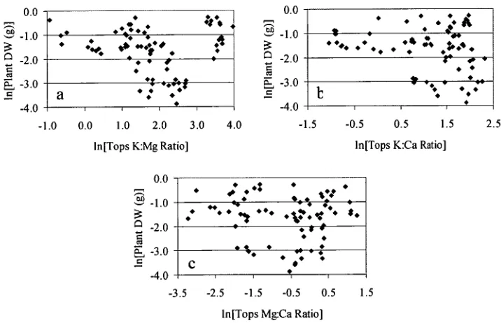
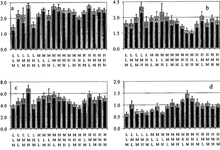
Figure 2.11. Relationships between Eucalyptus globulus plant dry weight and shoot nutrient ratios: (a) potassium-magnesium; (b) potassium-calcium; and (c) magnesium-calcium. Variables were transformed as appropriate. n = 81 55 Figure 2.12. Variation of leaf chlorophyll parameters with treatment: (a)
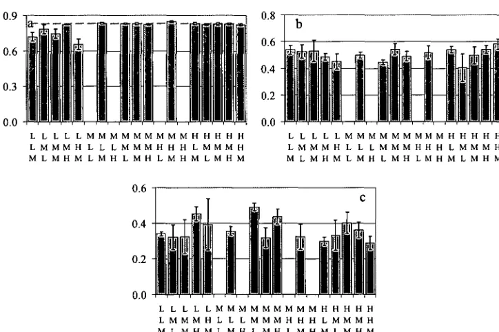
Figure 2.13. Variation of leaf fluorescence parameters with treatment: (a) Fv:Fm; (b) qP; (c) qN. For reference purposes, the common Fv:Fm value of 0.83 is indicated by a dashed red line. Error bars are s.e.m. 57 Figure 2.14. Variation of shoot base cation concentration with different
supplied magnesium and calcium concentrations: (a) potassium; (b) magnesium; and (c) calcium. Key: —*— Low calcium; —N— Medium calcium; —A— High calcium. Error bars are s.e.m. Points indexed with the same letter are not significantly different from each other. The larger, red point is the treatment that created the statistical interaction in the biomass data.
62
Figure 2.15. Variation of root base cation concentrations with supplied potassium and magnesium. The solid line in the botton left plot is the line of best fit to the relation. 69 Figure 2.B.1. Simplified response of chlorophyll to steps in measuring
fluorescence with a PAM, showing associated quantities, for dark adapted and light adapted plants. PQ = photochemical quenching; Non PQ =
non-photochemical quenching. Adapted from the Walz Mini-PAM Manual.
94
Figure 3.1. Variation of Pinus radiata dry weight with supplied (a) potassium; and (b) magnesium. The solid line represents the fitted curve; for comparison purposes, the dashed line represents the variation in Eucalyptus globus dry weight (see Figure 2.2).
103
Figure 3.2. Variation of Pinus radiata nutrient concentrations with supplied (a) potassium; and (b) magnesium. Legend: • Potassium; • Magnesium; •
Calcium; solid lines for shoot concentrations; dotted for root concentrations. 105 Figure 3.3. Variation of Pinus radiata root nutrient concentrations: (a)
magnesium with potassium; (b) calcium with potassium; (c) calcium with
magnesium. 106
Figure 3.4. Variation of Pinus radiata shoot nutrient concentrations: (a) magnesium with potassium; (b) calcium with potassium; (c) calcium with
magnesium. 107
Figure 3.5. Variation of Eucalyptus globulus shoot nutrient concentrations: (a) magnesium with potassium; (b) calcium with potassium; (c) calcium with
magnesium. 108
Figure 3.6. Variation of Pinus radiata shoot nutrient concentrations with root nutrient concentrations: (a) magnesium with potassium; (b) calcium with
potassium; (c) calcium with magnesium. 109 Figure 4.1. Configuration of a simple ion-selective electrode system. (After
Amman, 1996) 119
Figure 4.2. Calibration curves of Mg2+ and Ca2+ ion-selective microelectrodes. Electrodes were calibrated in standards, ranging from 50 to 500 mM. Electrode characteristics were as follows: Mg2+ LIX in Mg2+ standard: slope —
28.93 mV/decade, intercept -25.81 mV, correlation — 0.9994; Ca2÷ LIX in Ca2+ standard: -29.61 mV/decade, -7.98 mV, -0.9996; Mg2+ LIX in Ca2+ standard: -32.85 mV/decade, 8.01 mV, -0.9996.
126
Figure 4.3. Expected and calculated values for the magnesium concentration according to the concentrations of magnesium and calcium in the solution, in (1-1M).
129
Figure 4.4. Comparison of magnesium fluxes measured in 20011M Mg2+ in the presence of 2001.IM Ca2+calcium — calculated assuming no interference (triangles) and correcting for interference (closed circles) — and the absence of calcium (open circles). Negative values are net efflux.
Figure 4.5. Resolution of Na+ and K+ fluxesin responseto varioustypes of stresses by suggested method. a —transientfluxresponsesfrom Arabidopsis rootsin responseto hyperosmotic (200inM mannitol) stress. Fluxes were measuredinthe mature (4 mm fromthetip) zone of 8 d old roots. One representative example (out of 6)is shown. b — kinetics of Na+ and K+ flux responsesto ROS (1 mM copper ascorbate, Cu/A, added at 4 min). One representative example (out of 5)is shown. Negative values correspondto net ion efflux.
136
Figure 6.1. Average flux response of Eucalyptus globulus seedlingsto potassium stress applied att = 2 minutes: (a) K+, Apex; (b) K—, Apex;(c)
K+, Mature; (d) K—, Mature. Key: —N— Potassium; —*-- Magnesium; —A—
Calcium. Five plants pertreatment. Error bars are s.e.m (n = 5). Effluxis positive.
162
Figure 6.2. Average flux response of Eucalyptus globulus seedlingsto magnesium stress applied att = 2 minutes: (a) Mg+, Apex; (b) Mg—, Apex; (c) Mg+, Mature; (d) Mg—, Mature. Key: —N-- Potassium; —*— Magnesium;
—A— Calcium. Five plants pertreatment. Error bars are s.e.m (n = 5). Efflux
is positive.
163
Figure 6.3. Average flux response of Eucalyptus globulus seedlingsto calcium stress applied att = 2 minutes: (a) Ca+, Apex; (b) Ca—, Apex; (c) Ca+, Mature; (d) Ca—, Mature. In (b) and (d)the magnesium and calcium fluxes are plotted againstthe right-hand axis;the potassium ontheleft. Key: —.— Potassium; —*— Magnesium; —•— Calcium. Error bars are s.e.m (n = 5). Five plants pertreatment. Effluxis positive.
164
Figure 6.4. Average flux responseto salinity stress applied att = 2 minutes: (a) Eucalyptus globulus, apex; (b) Eucalyptus globulus, mature; (c) ET8, apex; (d) ET8, mature. In (a) and (c)the Mg and Ca fluxes are plotted against the right hand axes. Key: —N— Potassium; —•— Magnesium; —•— Calcium. Five plants pertreatment. Error bars are s.e.m (n = 5). Effluxis positive.
165
Figure 6.5. Relationships between Eucalyptus globulus net fluxes: (a) magnesium and potassium; (b) calcium and potassium; (c) calcium and
magnesium. The solidlinesinthe plots arethe regressions shownintable 6.4. 167 Figure 6.6. Relationships between Eucalyptus globulus net potassium and
magnesium fluxes forthetreatments: (a) K+; (b) K—; (c) Mg+; (d) Mg—; (e) Ca+; (f) Ca—; (g) Salt (Euc); (h) Salt (Wheat). The solidlineinthe plot are the regressions shownintable 6.5.
171
Figure 6.7. Relationships between Eucalyptus globulus net potassium and calcium fluxes forthetreatments: (a) K+; (b) K—; (c) Mg+; (d) Mg—; (e) Ca+; (f) Ca—; (g) Salt (Euc); (h) Salt (Wheat). The solidlinein (d)isthe regression shownintable 6.6.
172
Figure 6.8. Relationships between Eucalyptus globulus net magnesium and calcium fluxes forthetreatments: (a) K+; (b) K—; (c) Mg+; (d) Mg—; (e) Ca+; (f) Ca—; (g) Salt (Euc); (h) Salt (Wheat). The solidlineinthe plot are the regressions shownintable 6.7.
173
Figure 7.1. Fragment of record of oscillatory H+ flux around a root ofTriticum aestivum cv. "Machete" measured at — 21 mm fromthe apex. The solidlineis a simple sine function for comparison. Effluxis positive. 188 Figure 7.2. Fragments of records of oscillatory fluxes aroundthe roots of: (a)
Triticum aestivum cv. "ET8"; and (b) Eucalyptus globulus. Effluxis positive.
Figure 7.3. Two fragments of a record of Fr fluxes measured simultaneously at three different locations along the same root of Triticum aestivum cv. "Machete". The measurements were taken at 2.3 mm (triangles); 3.5 mm (squares); and 4.7 mm (diamonds). Efflux is positive.
Figure 7.4. Fragment of a record of Fl÷ fluxes measured simultaneously at three different locations along the root of Eucalyptus globulus. The measurements were taken at 0.23 mm (triangles); 1.40 mm (squares); and 2.30 mm (diamonds). Efflux is positive.
190
Table of Tables
Table 2.1. Soil solution concentrations of unfertilised forestry plantations
(from Mitchell & Smethurst, 2004) 31 Table 2.2. Treatments and concentrations used in the single and two-factor
experiments. 33
Table 2.3. Chemicals used in nutrient solutions for the base cation response
experiments. 34
Table 2.4. Significant dates in the experiments. 34 Table 2.6. Variation of average shoot and root K, Mg and Ca concentrations with the supplied concentration of that base cation. The second column details the supplied concentration of the cation of interest: Low = 10 uM; Medium = 500 uM; and High = 5,000 uM. Errors are s.e.m. All treatments for a given cation are significantly different at 1%. n = 37 for each treatment.
48
Table 2.7. Regressions of the root cation concentrations on the supplied concentration. The symbols KRoot, MgRoot, and CaRoot are the concentrations of
the cations in the roots in % per unit dry weight; and K w., mgsoh„ and Casoin are the supplied concentrations, in ?AM. The values r are the Pearson
correlation coefficients, with the significance determined for n = 81.
50
Table 2.8. Correlation between root concentrations of the base cations. The values r are the Pearson correlation coefficients, and the significance
determined for n = 81. 51
Table 2.9. Correlation between shoot and root concentrations. The values r are the Pearson correlation coefficients, and the significance determined for n = 81 52 Table 2.10. Correlation between plant dry weight and tops base cation
concentrations, transformed to provide the highest correlation. The values r are the Pearson correlation coefficients, and the significance determined for n = 81 52 Table 2.11. Correlation between the supplied base cation concentrations and root cation concentrations. From the information in Section 2.3.4, the natural logarithms of both the ratios and concentrations were used. The values r are the Pearson correlation coefficients, and the significance determined for n = 81.
54
Table 2.12. Correlations of base cation ratios throughout the plant: the root ratios against the solution ratios; the shoot ratios and the root ratios; and the shoot ratios and the plant dry weight. The symbols K:Mg, K:Ca and Mg:Ca are the appropriate cation ratios; DW is the plant dry weight; and the subscripts "Soln", "Root"; and "Shoot" indicate that the ratios are measured in the supplied solution, the root or the shoot, respectively. The values r are the Pearson correlation coefficients, and the significance determined for n = 81.
55
Table 2.A.1. Differences between treatments: plant dry weights. Superscript letters refer to pairs of apparently contradictory effects. Comparison of pair "a" shows that there was no significant difference between the two treatments (t = 1.559, 34 DoF), nor was their average significantly different from zero (t = 0.831, 35 DoF).
84
Table 2.A.2. Chla content, differences between treatments. Superscript letters refer to pairs of apparently contradictory effects. Comparison of the pair "a" shows that these two results are significantly different (t = 3.778, 34 DoF, 1%), which means that it is not possible to combine them to draw an overall
conclusion. Comparison of the pair "b" shows that these two results are not significantly different (t = 0.514, 34 DoF), nor is their average significantly different from zero (t = 1.099, 35 DoF).
Table 2.A.3. Chlb Content, differences between treatments. Superscript letters refer to pairs of apparently contradictory effects. Comparison of the pair "a" shows that these two results are not significantly different (t = 1.285, 34 DoF), nor is their average significantly different from zero (t = 0.676, 35 DoF). Comparison of the pair "b" shows that these two results are not significantly different (t = 0.875, 34 DoF), nor is their average significantly different from zero (t = 0.560, 35 DoF).
86
Table 2.A.4. Total Chl Content, differences between treatments. Superscript letters refer to pairs of apparently contradictory effects. Comparison of the pair "a" shows that these two results are not significantly different (t = 1.285, 34 DoF) from each other, nor is their average significantly different from zero (t = 0.676, 35 DoF).
87
Table 2.A.5. Chla:Chlb Ratio, differences between treatments. Superscript letters refer to pairs of apparently contradictory effects. Comparison of the pair "a" shows that these two results are significantly different (t = 4.949, 34 DoF,
1%) from each other so it is not possible to draw a conclusion about an over-all effect. Comparison of the pair "b" shows that these two results are
significantly different (t = 1.728, 34 DoF, 5%) from each other so it is not possible to draw a conclusion about an over-all effect. Comparison of the pair "c" shows that these two results are not significantly different (t = 1.574, 34 DoF) from each other, nor is their average significantly different from zero (t =
1.000, 35 DoF). Comparison of the pair "d" shows that these two results are not significantly different (t = 0.601, 34 DoF) from each other, nor is their average significantly different from zero (t = 0.991, 35 DoF).
88
Table 2.A.6. Fv:Fm ratio, differences between treatments. Superscript letters refer to pairs of apparently contradictory effects. Comparison of the pair "a" shows that these two results are significantly different (t = 4.345, 34 DoF, 1%) from each other so it is not possible to draw a conclusion about an over-all effect.
89
Table 2.A.7. Photochemical quenching fraction, qP, differences between
treatments. 90
Table 2.A.8. Non-photochemical quenching fraction, differences between
treatments. 91
Table 2.C.1. Eucalyptus spp. foliar base cation concentrations. Values are from field grown experiments, unless marked with an asterisk (hydroponic), or
dagger (soil in pot). 95
2.D.1. The concentrations of supplied potassium, magnesium and calcium,
along with the numbers of plants in each of the replicates of those treatments. 95 Table 3.1. Treatments and concentrations used in the Pinus radiata
single-factor experiments. Note that there were two replicates of each treatment. 100 Table 3.2. Chemicals used in nutrient solutions base cation response
experiments. 102
Table 3.3. Significant dates in P. radiata the plant response experiments. 102 Table 3.4. Regressions of the root cation concentrations on the supplied
concentration. The symbols KRoot, and MgRoot are the root concentrations of the
cations; and Ksoln, and Mgs„,„ are the supplied concentrations. The values r are the Pearson correlation coefficients, and the significance determined for n = 12 and n = 10 for potassium and magnesium, respectively.
104
Table 3.5. Correlation between root concentrations of the base cations. The values r are the Pearson correlation coefficients, and the significance
Table 3.6. Correlation between shoot concentrations of the base cations. The values r are the Pearson correlation coefficients, and the significance
determined for n = 22. 107 Table 3.7. Correlation between shoot concentrations of the base cations in
Eucalyptus globulus. The values r are the Pearson correlation coefficients, and the significance determined for n = 81. 108 Table 3.8. Correlation between shoot and root concentrations. The values r are the Pearson correlation coefficients, and the significance determined for n = 22. 109 Table 3.9. Foliar potassium and magnesium concentrations, with associated
visual deficiency symptoms and foliar ratio, from field-grown Pinus radiata.
From Adams (1973) 115
Table 3.A.1. Pinus radiata base cation concentrations. Values are from field grown experiments, unless marked with an asterisk (hydroponic), or dagger
(soil in pot). 117
Table 4.1. Calculated magnesium concentration of sample solutions of known magnesium concentration containing various concentrations of the interfering ion calcium. The first two columns show the supplied concentrations of magnesium and calcium in the samples, respectively. The third column shows the amount of magnesium calculated to be in the sample solution based upon the response of the MIFE system.
125
Table 4.2. The accuracy of the Nicolslcy-Eisenman equation (5) in predicting the voltage response of ion-selective membrane electrodes in the presence of an interfering ion. Samples (n = 4) containing known concentrations of Mg and Ca were measured using MIFE, the measured voltage being compared with the expected response calculated with equation 8 using the known Mg and Ca concentrations. Column "Fraction" = theoretical response ÷ actual response.
128
Table 6.1. Solutions used in stress-induced flux measurements. The treatments were applied as described in Section 6.2.3. The manufacturers of the chemicals are as in table 2.2.2. 155 Table 6.2. Chemicals used to make up ion-selective micro-electrode
calibration solutions 156
Table 6.3. Initial flux values used in plots of plant response to stress. The
errors are s.e.m., with n = 12 plant samples. 158 Table 6.4. Correlation between pre-treatment net ion fluxes. The values r are
the Pearson correlation coefficients, and the significance determined for 4,071
pairs. 166
Table 6.5. Correlation between net potassium and magnesium ion fluxes following potassium addition (K+) & removal (K—); magnesium addition (Mg+) & removal (Mg—); calcium addition (Ca+) & removal (Ca—); and salinity stress to Eucalyptus globulus (Euc) & Triticum aestivum (Wheat). The quantities K+ & Mg2+ in the regression refer to the net fluxes of those ions.
168
Table 6.6. Correlation between net potassium and calcium fluxes following potassium addition (K+) & removal (K—); magnesium addition (Mg+) & removal (Mg—); calcium addition (Ca+) & removal (Ca—); and salinity stress to Eucalyptus globulus (Euc) & Triticum aestivum (Wheat). The quantities K+ & Ca2+ in the regressions refer to the net fluxes of those ions.
169
Table 6.7. Correlation between net magnesium and calcium fluxes following potassium addition (K+) & removal (K—); magnesium addition (Mg+) & removal (Mg—); calcium addition (Ca+) & removal (Ca—); and salinity stress to Eucalyptus globulus (Euc) & Triticum aestivum (Wheat). The combined regression of the + / — data is given at +/-. The quantities Mg2+ & Ca2+ in the regressions refer to the net fluxes of those ions.
Table 7.1. Mean values (nmol 111-2 S-1) of net fl+ oscillations at different electrode locations in the elongation zone of "Machete" wheat root. Data are mean ± s.e. (n = 6-8). Differences marked with ** indicate significance at the
1% level. Influx is positive.
Table 7.2. Periods of net H+ oscillations at different electrode locations in the elongation zone of "Machete" wheat root. Data are mean ± s.e. (n = 6-8). Differences marked with * or ** indicate significance at the 5% or 1% level, respectively
191
1. Introduction
In forestry, as in all agricultural cropping activities, adequate nutrition is essential to ensure adequate growth and consequent economic returns. The causes of inadequate nutrition are manifold, including site-factors, silvicultural practices, and plant-specific characteristics.
In Europe and north-eastern North America, new forms of forest "die-back" are being associated with soil magnesium, potassium and calcium deficiencies, often in conjunction with acid soils (Hannick,
etal.,
1993; Hattl, 1988). In South Africa, the soils are often extremely infertile, lacking in most of themacronutrients (Schonau & Herbert, 1983). New Zealand, a country with extensive forestry estates, has soil that is abundant in both potassium and magnesium, yet the magnesium is in a form that is unavailable to plants (Will,
1961b; Hunter, et al., 1986); this has been implicated in the potentially
productivity-reducing condition of Pinus radiata known as "Upper Mid-Crown Yellowing" (Beets & Jokela, 1994). In Australia, also, the age of the soil and the relatively intensive cropping of the existing plantations, have led to concerns about their current and future health (Wong & Harper, 1999; Mitchell & Smethurst, 2004).
Poor choice of site is often a contributing factor to base cation deficiency (Shedley, et al., 1993). Traditionally, in Australia and New Zealand, forestry plantations have been established on land that is not already used for agriculture (Boomsma & Hunter, 1990; Birk, 1994); that is, they are established in regions with poor soil, low rainfall, extreme temperatures, or even all of the above. This problem has been addressed, to an extent, in recent times, with a proportion of plantations being established on ex-farmland (Boomsma & Hunter, 1990).
1997); the concentrations of magnesium and calcium were lower, but of potassium and nitrogen higher, in the soil under Pinus radiata when compared with Eucalyptus regnans on similar sites in NZ (Jurgensen, et al., 1986); while under Pinus radiata in New South Wales, the concentrations of nitrogen and magnesium were lower than under nearby native eucalypts (Turner & Lambert,
1988). In addition, changes in topsoil acidity have been observed under forested sites (Parfitt, etal., 1997; Adams, etal., 2001), which directly affects that
availability of nutrients (Marschner, 1995), and also increases the concentration of toxic aluminium species in the soil (Adams, et al., 2001; Godbold & Jentschke,
1998; Kinraide, etal., 1992).
Even if the site chosen for plantation establishment has adequate nutrition, low rainfall is enough to induce base cation deficiency because soil moisture is
necessary to allow plants to access nutrients within the soil (Zeng & Brown, 2000; Turner, 1982; Lambert & Turner, 1988; Sands & Mulligan, 1990). The two major vectors for delivery of nutrients to the root surface are bulk flow and diffusion (Smethurst, 2000). Practically, all of the three base cations potassium, magnesium and calcium can be delivered by either vector but, for potassium diffusion is more common, for calcium mass flow is more common, and magnesium seems to have no preferential mode (Ohno & Grunes, 1985; Marschner, etal., 1991).
Removal of plant material from plantations, whether it be because of harvesting, thinning, or litter removal, removes nutrients and disturbs the natural nutrient cycles (Smith, etal., 1994; Watmough & Dillon, 2003). Some site preparation practices also contribute to nutrient loss; for example, burning the post-harvest litter adds large quantities of nutrients to the soil, but some of these nutrients are readily leached and lost (Zwolinski, et al., 1993). Clearly, if the rate of nutrient removal is greater than the rate of replenishment from mineral weathering, atmospheric input or fertilisation, a deficit will eventually develop.
directly leach cations from foliage (Hail, et al., 1990; Schaberg, et al., 2000). Further, excess protons within the acid rain, and Al 3+ released from the soil by the increased acidity, passing through the soil exchange with cations adsorbed to the organic matter and clay in the soil matrix, causing base saturation to decrease and increasing the likelihood of leaching (Svedrup & Rosen, 1998; Minocha, et al., 1997). Moreover, the aluminium directly competes with, and inhibits the uptake of base cations, especially magnesium and calcium (Godbold et al., 1998; Kinraide, etal., 1992; Ericsson, etal., 1995; Ericsson, etal., 1998).
Fertilisation with other base cations, not necessarily to excess, is, ironically, another of the causes of base cation deficiency (Snowdon & Waring, 1985). By adding cations to the soil, the equilibrium that previously existed within the soil system is altered towards a new equilibrium, and ions other than the species added may be freed from the soil matrix and liable to be leached. For example, adding calcium has been observed to free up potassium and magnesium; adding
potassium frees up calcium and magnesium (Johns & Vimpany, 1999; Aitken, et al., 1999; Seggewiss & Jungk, 1988); and adding nitrogen in the form of NH4 ± frees up potassium, magnesium and calcium (Snowdon & Waring, 1985). Adding nitrogen as NI-I4 has the added effect of acidifying the soil, further altering the accessibility of the nutrients (Smethurst, et al., 2001; Mitchell & Smethurst, 2004).
Nutrient deficiency in plants is sometimes brought about by competition with other ions (Marschner, 1995). In such cases, uptake of a nutrient (e.g.
1985). The most obvious location for interaction is at the plasmalemma, where the ions compete for binding sites of trans-membrane carriers (Troyanos, et al., 2000; Diem & Godbold, 1993), yet it has been suggested that the interaction between potassium and magnesium, at least, occurs somewhere in the
translocation of these nutrients from the roots to the shoots (Ohno & Grunes, 1985; Diem & Godbold, 1993). Now, since the presence of a nutrient can interfere with the uptake of another nutrient, it follows that the ratio of these nutrients may have an effect on the nutritional status of the plant (Hewitt, 1963; Ericsson etal., 1998; Schonau, 1982; Schonau & Herbert, 1983), with the implication that an excess of one can induce a deficiency of the other.
There are many indicators used for inferring sub-optimal nutrition. The most straight-forward of these is simply the dry weight of the plant: if the dry weight of the plant is not maximal, and all other environmental factors are within the bounds required for normal growth, nutrition must be inadequate. It should be noted, however, that dry weight is a crude measure, providing little information as to the missing nutrient(s). Foliar symptoms may provide an indication of nutrient deficiency, and may even be used to identify the deficient nutrient (see, for example, Marschner, 1995). But, usually, by the time that symptoms are apparent, the deficiency is severe. Moreover, some species, in particular Eucalyptus, are somewhat reticent in displaying deficiency symptoms, making foliar deficiency symptoms a less than ideal method of diagnosis.
An alternative approach to inferring nutrient deficiency is to ascertain the nutrient availability in soil in which the plants are growing. Various methods have been used in agriculture (for example, acid, alkaline or salt extracts) to indicate a nutrient deficiencies (Peverill,
et al.,
1999), and are occasionally used in plantation forestry (for example, Ballard & Pritchett, 1975). A drawback with these methods is that different extraction methods provide different values for any given nutrient (for example, Mendham,et al., 2002), and extensive
soil-crop-climate-specific calibrations are needed. The concentration of nutrients in soil solution has also been suggested as a potential indicator of nutrient deficiency (Smethurst, 2000), an approach that has met with some success in forestry because it is more mechanistic and is therefore of potentially of more broad applicability and requiring less extensive calibration (for example, Mendham, etal., 2002).
Ultimately, nutrient uptake, measurable as an ion flux, is at a cellular level and, in response to changing local conditions, ion fluxes can vary in magnitude and direction on a time scale of minutes (for example, Shabala & Knowles, 2002; Newman, 2001). Since trans-membrane ion transport processes are central to the regulation of plant homeostasis and adaptation (Zimmerman,
etal.,
1999;Shabala, 2003b), observation of such can provide information about root, and therefore plant, adaptive behaviour, whence indications of suitability of
environmental or nutritional conditions, which indications can be subsequently investigated on a larger scale. Using nutrient concentrations in gross plant organs can lead to errors in interpretations as they are, effectively, the net sum of all cellular fluxes since the germination of the seed. Rates of uptake, therefore, can be only crudely ascertained and interactions between nutrients can only be inferred. Using radio-isotopes shortens the integration period, but is still a
"bottom line" picture. Since the advent of easily fabricated liquid-membrane ion-selective micro-electrodes in the late 1980s (for example, Newman,
et al.,
1987; Kiihtreiber & Jaffe, 1990; Kochian,et al.,
1992), it has been possible tomechanisms behind ion fluxes (Shabala & Knowles, 2002; Shabala L, et al., 2005; Newman, 2001).
There are currently commercially available ionophore "cocktails" that permit the measurement of a wide range of ions in solution; for example, NH4+, Ca2+, Cr, H+, Mg2+, NO3-, K+, and Na+ (Fluka, 2007). In addition, it is possible to
manufacture ionophores when such are not available commercially. For various chemical reasons, the ionophores available for use as ion-selective membranes are usually cations, with the most relevant to plant nutrition studies being hydrogen, potassium, calcium, magnesium and sodium, all of which are available in as proprietary cocktails. To date, ion-selective membranes, whether solid or liquid, for the latter two ions have the unfortunate property of being not exclusively selective: the magnesium-selective electrodes respond strongly to
the presence of
calcium, and the sodium-selective electrodes to potassium, although the converse reactions do not hold. This behaviour was identified in the first half of the 20th century by Nikolsky and a mathematical correction method formalised by Eisenman in the 1950s (Koryta, 1972). This method is, however, stillcontroversial, in that the International Union of Pure and Applied Chemists hold that the Nikolsky-Eisenman method works well (Macca, 2003) in spite of evidence to the contrary (Ren, 1999, 2000; Zhang, et al., 1998).
The purpose of the experiments presented in this thesis was to investigate the effects of differing solution concentrations of the base cations potassium,
To provide more information about the mechanisms of nutrient uptake, the net ion fluxes of potassium, magnesium and calcium around the roots of Eucalyptus globulus were measured using MIFE technology, which provides real-time ion flux measurements with a high spatial and temporal resolution, of the orders of micrometres and seconds, respectively. Initially, to enable the simultaneous measurement of magnesium and calcium fluxes, the problem of ion selectivity was addressed. Once resolved, the net flux patterns around Eucalyptus globulus roots were measured in response to various stresses, including salinity, to provide an indication of uptake mechanisms. For comparison purposes, because the base cation fluxes of Eucalyptus spp. have not been previously recorded', seedlings of the well-studied species Triticum aestivum were also subject to salinity stresses.
2. Effects of Base Cation Concentrations and Ratios on
the Dry Weight, Nutrient Concentrations and Ratios, and
Fluorescence Parameters of
Eucalyptus globulus
seedlings.
2.1. Introduction
Adequate nutrition is one of the major factors in plant growth. Early diagnosis of a base cation deficiency (indeed, any nutrient deficiency) is, therefore, desirable so that poor growth can be corrected by fertiliser application. In hardwood and softwood plantations in both Australia and New Zealand there are persistent concerns about the availability of the base cations potassium, magnesium and calcium (Khanna, 1997). These concerns are based on cation budgets (for example, Judd, 1996; Webber & Madgwick, 1983), some cases of confirmed K deficiency in pines and eucalypts (for example, Raupach & Hall, 1971; Turner & Lambert, 1986; Mitchell & Smethurst, 2004; Smethurst, et al., 2007), suspected wide-spread magnesium deficiency in pines (Hunter, 1996; Payn, et al., 1995), and calcium deficiency in pines (Turner & Lambert, 1986). Moreover, the projected increased usage of nitrogen fertilisers is expected to increase crop demands for cations (Smethurst, et al., 2001; 'Oiling, et al., 1997; Claasen & Wilcox, 1974) and increase cation losses through leaching (Mitchell & Smethurst, 2004; Grimme & Nemeth, 1975; Milling, et al., 1997). It is very likely,
therefore, that serious cation deficiencies will manifest during the current or future crop cycles.
The existing knowledge base for managing such a situation is limited. There are no reliable soil diagnostics (Smethurst, 2000), and few plant-based diagnostics (especially in Eucalyptus species) to enable prediction of a cation deficiency. Furthermore, field-based fertilisation trials have displayed inconsistent responses to base cation addition (for example, Merino, etal., 2003; Shedley, et al., 1993;
If it is assumed that healthy plants require a certain minimum level of a given nutrient, and that this level will be reflected in the concentrations of that nutrient in plant organs (Ellis & van Laar, 1999; Ingestad & Lund, 1986), then measuring the concentration of nutrients in plant organs can indicate which nutrients are lacking. Moreover, nutrient content information can be obtained at a very early stage in plantation development, allowing prompt intervention. This approach has been used successfully to identify nutrient deficiencies in forests (for example, Lambert & Turner, 1988; Bell & Ward, 1984a; Schonau, 1981a & b; Jones & Dighton, 1993).
Another approach to determining nutrient deficiency in plants is to ascertain the concentrations of nutrients in the soil (Payn & Clough, 1987; Smethurst, et al., 2001; Turner & Lambert, 1987). While this approach cannot precisely diagnose the deficient nutrient in the plant (Ellis & van Laar, 1999), it can provide a very good indication of the likely suspect. Further, it can be used before plantation establishment to identify sub-optimal nutrients and apply early correction.
Measuring various chlorophyll fluorescence parameters of leaves is a relatively simple, and increasingly common, method of ascertaining whether crops are under stress (Maxwell & Johnson, 2000; Smethurst & Shabala, 2003). Detectable changes in these parameters, caused by a variety of stresses, have been observed in both annual and perennial crops; for example, Medicago sativa in response to waterlogging, Lycopersicon esculentum in response to chilling stress and nutrient deficiency, Pinus radiata in response to salinity and nutrient deficiency, and Eucalyptus pauciflora in response to chilling stress and elevated CO2 (Smethurst & Shabala, 2003; Starck, et at, 2000; Sun, et al., 2001; Roden, et at 1999).
Efficient use of fertiliser to correct nutrient deficiency relies on calibration between the amount of nutrient in the soil and resultant growth, but few calibrations are available for forest plantations (Smethurst, 2000). There are several reasons for this. While it is relatively simple to determine the concentrations of some forms of individual nutrients in soil, it is difficult to ascertain the quantities that are actually available to plants (Hunter, et al., 1986). All methods provide only an indirect measure of the concentrations of the
available forms that occur at the root surfaces (Rengel & Marschner, 2005;
Hunter, et al., 1986) and, indeed, different methods may provide different answers (for example, Adams, 1973). While the paste method of Smethurst and
co-workers is helpful in this regard, interactions of base cations at root surfaces are not accounted for (Smethurst, 2000). Due to the complex chemical interactions that occur within the soil matrix, it is difficult to predict the end effect of
fertilisation. For example, the addition of nitrogen fertilisers can lead to increased base cation availability and, consequently, leaching susceptibility (Mitchell &
Smethurst, 2004); similarly, the addition of magnesium can increase soil solution potassium, and vice versa (Grimme & Nemeth, 1975). Furthermore, each soil responds differently to fertilisation according to its chemical, physical and
biological characteristics. In consequence, soil-based fertiliser trials, upon which much growth-response data is based, are prone to misinterpretation.
The growth rate of plants is often limited by their rate of nutrient uptake
(Ingestad, 1982; Ericsson & Kahr, 1995), a primary determinant of which is the concentration of nutrient in the liquid phase (solution) that can be maintained at the surface of the roots of the plant (Zeng & Brown, 2000; Sands & Mulligan,
Since background knowledge about the base cation requirements of Eucalyptus species was limited, an experiment was conducted to investigate the effects of differing concentrations of supplied cations on the growth of Eucalyptus globulus. At the end of the growth experiments, various leaf fluorescence parameters were measured, the leaf chlorophyll concentrations ascertained, and the shoots and roots were analysed to determine the concentrations of base cations in those parts. These data were compared with the growth data to investigate links between physiological and gross plant parameters.
2.2 Materials and Methods
2.2.1. Base Cation Concentrations
The concentrations at which the base cations potassium, magnesium and calcium were supplied were based on: (1) typical concentrations of those nutrients in soil solutions in samples from Australian plantation sites (Mitchell & Smethurst, 2004); (2) typical concentrations found in highly fertile and fertilised soils or hydroponic solutions (for example, Hoagland's number 2); and (3) the minimum concentrations likely to be required to ensure a net uptake. Using the
concentrations found in soil solutions (as opposed to other methods of assessing soil fertility) was suggested by Smethurst (2000) as a potential indicator of
nutrient deficiency, and the approach was demonstrated to be useful for predicting the likelihood of N and P deficiency in eucalypt plantations (Mendham, et al., 2002; Smethurst, et al., 2004), and K deficiency in Pinus radiata plantation (Smethurst, et al., 2007).
information about plant responses to intermediate concentrations of supplied nutrients.
Plant dry weight was chosen as the indicator of nutrient effectiveness. While dry weight is less sophisticated than other indicators, it provides a straightforward assessment of environmental suitability: the best conditions give the best growth. Moreover, dry weight is the most relevant to forestry, where the size of the tree is important.
Concentrations of other nutrients in the growth solution were generally as per half-strength Hoagland's #2 growth solution. The level of nitrogen as NH4 was significantly higher than as NO3, because it has been found that Eucalyptus globulus and Eucalyptus nitens have a preference for NH4 over NO3 (Garnett &
Smethurst, 1999; Shedley, et al., 1993). On the other hand, phosphorus was supplied at a much reduced level, as Eucalypts are known to be intolerant of high phosphorus (Thomas, 1981), and maximal growth of Eucalyptus globulus had been obtained with a soil solution phosphorus concentration of less than 1 pM (Smethurst, 2000). Finally, since the solutions were prepared with the chloride salts of potassium, magnesium and calcium, the solution chloride concentration was greater than that in a standard half-strength Hoagland's #2. As chloride toxicity is generally linked with elevated sodium concentrations and, in the
growth solutions sodium was kept to a minimum, the high chloride concentrations were assumed to be non-toxic.
Site Potassium (gM) Magnesium (j-im) Calcium (I.J.M) pH
Westfield 170 90 90 4.6
Tim Shea 120 60 50 5.0
Nunamara 140 13 250 6.0
Penna 240 60 540 7.0
Nicholas 150 90 80 4.2
BFG 160 80 270 5.7
Imbil 300 220 450 7.1
2.2.2. Plant Culture
Two sets of experiments were performed. One was a set of three two-factor experiments to test for gross concentration and ratio effects; the other, a set of two single-factor experiments to more closely investigate the effects of potassium and magnesium concentrations.
Eucalyptus globulus was chosen as the subject because it is a major plantation forestry species in Australia, with plantations comprising 21% of the 1.7 million hectare national plantation forestry estate. By comparison, Eucalyptus nitens, the next most common plantation forestry hardwood species, and Pinus radiata, the most common plantation softwood, comprise 2%, and 49%, of the national estate, respectively. (Anon, 2005).
Eucalyptus globulus seeds (Boral seed orchard, Tin-01001, supplied courtesy of Bill Neilsen, Forestry Tasmania) were placed on moistened paper towels. These were then rolled loosely and placed to stand end-on in a 10 1 plastic container with tap water to a depth of 20 mm. The container was covered to reduce evaporation and placed in a darkened, temperature controlled growth cabinet held at 21 °C. The seeds germinated within four days and, by fourteen days, were large enough to plant out into the hydroponic units.
Each hydroponic culture unit consisted of a 5 1 capacity plastic container, with the sides and bottom covered with a layers of black plastic film to minimise the amount of light reaching the seedling roots. A grid made of opaque white "Handiboard" (Laserlite, Australia) was cut to fit into the top of the plastic
The hydroponic units were topped up once per day with single distilled water to compensate for evaporation, and completely changed every fourteen days during the first month after seedling transfer, and once every seven days thereafter. The solutions were aerated after the first solution change (prior to this the delicate seedling roots would have been damaged by the turbulent water) by means of an "air-stone" (of the type used in aquaria) connected by silicon tubing to air manifolds supplied by an electric air pump (Gast Manufacturing Co., Benton Harbour, Michigan).
The experiments were performed in a climate-controlled greenhouse with the temperature held at approximately 24°C between 0700 and 1900, and
approximately 15°C for the remainder of the day. Supplementary lighting was not supplied.
Each experiment in the two-factor series was set up as a complete, randomised block design, two-factor, complete factorial experiment, with each factor having three levels, and each level having three replicates. In each of the experiments, one of the base cations was held at a concentration of 500 JAM, while the
concentrations of the other two base cations were supplied at either 10 i_tM, 5001.1M, or 50001AM (referred to hereafter as "low", "medium", or "high", respectively). There were also two single-factor experiments, with each factor having five levels and each level having two replicates. Details of the treatments and concentrations are set out in Table 2.2; the number of plants, and the
concentration of chloride in each treatment is given in Appendix 2.D to this chapter.
Variables Potassium (i.tM) Magnesium (gM) Calcium (gM) Mg-Ca
K-Mg K-Ca
Mg
500 10 / 500 / 5000 10 / 500 / 5000 20/40 /80/
160 / 320
500
10 / 500 / 5000 10 /500 /5000
500
500
20/40/80/ 160 / 320
10 / 10 / 500 / 500 500 / 500 500 5000 5000
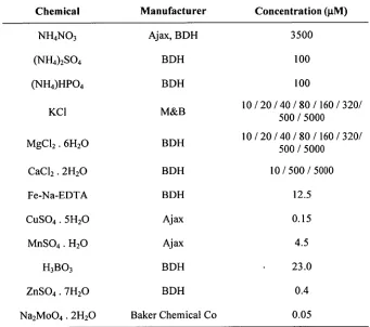
The nutrient solution was made by adding sufficient stock solution, prepared from analytical grade reagents,to single-distilled waterto providethe required final concentrations. The chemicals used,the manufacturers, andthe concentrations usedinthe experiments are shownin Table 2.3.
The experiments were run sequentially between spring, 2001, and mid-summer 2002/3. The exact dates are shownin Table 2.4.
Chemical Manufacturer Concentration(gM)
NH4NO3 Ajax, BDH 3500
(NH4)2SO4 BDH 100
(NROHPO4 BDH 100
KCI
MgC12. 6H20 CaC12. 2H20 Fe-Na-EDTA CuSO4. 5H20
MnSO4. H20 H3B03 ZnSO4. 7H20 Na2Mo04. 2H20
M&B
BDH BDH BDH Ajax Ajax BDH BDH Baker Chemical Co
10 /20/40/80 /160 /320/ 500 / 5000
10 /20 /40/80 /160/320/ 500 / 5000
10 /500 /5000 12.5 0.15 4.5 23.0
0.4 0.05 Table 2.3. Chemicals usedin nutrient solutionsforthe base cation response experiments.
Commencement Transfer to Duration Experiment Date Hydroponics Harvest Date (days)
[image:33.562.123.464.231.533.2]2.2.3. Plant Dry Weight Determination
At the end of each experiment the plants were removed from the nutrient solution and prepared for analysis. To ensure sufficient material for analysis, individual plants within replicates (each growth unit) were pooled. The shoots were excised with sharp scissors and the roots were blotted dry with paper towel to remove excess water. Dry weights were recorded after drying at 75°C for seven days.
2.2.4. Nutrient Content Analysis
Plant material, dried as in section 2.2.3, was ground and stored in glass vials. Prior to the acid digest, the samples were dried for at least 24 hours at
approximately 75°C, then cooled in a desiccator. Sub-samples (0.16 g ± 0.005 g) were transferred to clean, dry 50 ml glass digest tubes, with three blank samples and three quality control samples included in each set of digests. The digest followed Lowther (1980). The dilute samples were stored in clean, airtight bottles. Analysis for potassium, magnesium and calcium was performed using a Varian SpectrAA-400 flame photometer following the protocol set out in the manual for the instrument (Varian, 1989).
2.2.5. Chlorophyll Fluorescence
A brief overview of leaf chlorophyll fluorescence theory and a statement of the equations used in calculating fluorescence parameters is in Appendix 2B to this chapter.
Leaf chlorophyll fluorescence was measured with a Walz Mini-PAM portable fluorometer equipped with a 2030-B leaf-clip holder incorporating integrated micro-quantum and temperature sensors (Mini-PAM, Heinz Walz GmbH,
Fluorescence measurements on dark adapted plants were made approximately one hour after sunset, which is long enough for the plants to be truly dark-adapted (Rohkek & Bartak, 1999). Five measurements were made per treatment
replicate, each on one of the youngest pair of fully expended leaves of a randomly chosen plant within the replicate. The Fo value was measured under a low
irradiance (0.15 ilmol photons m -2 s-1) modulated measuring beam, and Fm was induced by a 0.8 s pulse of saturating white light.
Fluorescence measurements for light adapted plants were made during the mid-afternoon when the ambient light was relatively constant. Three measurements were made per treatment replicate, each on one of the youngest pair of fully expended leaves of a randomly chosen plant within the replicate. Actinic light at an intensity of approximately 250 i.tmol photons M-2 s-1 (photosynthetically active
radiation) was applied for sufficient time that the Ft value was stable, and a saturating pulse, as for the dark-adapted plants, was applied to obtain Fm'.
The fluorescence parameters calculated for each plant were pooled so that each treatment within an experiment had at least five replicates; from this data-set a random subset of five replicates per treatment was chosen for statistical analysis.
2.2.6. Leaf Chlorophyll Content
Following harvest, leaf chlorophyll extraction and determination were performed following the protocol described in Smethurst & Shabala (2003). Five small samples from each treatment were taken, such that each methanol extraction vial contained between 0.08 g and 0.15 g of leaf material.
2.2.7. Data Analysis
Normalisation and Combination of Two-factor Treatments for Presentation
normalisedtreatmentsthat are presentedinthe plots were recalculated fromthe normalised data.
Critical Cation Concentration
The critical base cation requirements, beingthe concentration of base cationinthe nutrient solution necessaryto provide growth at 90% ofthe calculated maximal rate, were obtained by solvingthe Michaelis-Menten equation forthe value ofthe nutrient at whichthe growth parameter was 90% ofthe maximum:
ax
y = 0.9a = —> 0.9(b + x) = x —> x = 9b. b+ x
Thatis,the value at which xis 90% ofthe maximum valueis ninetimesthe Michaelis-Menten rate content (the coefficient bin equation 3, above).
Investigation of Ratio Effects
Two different styles of ratio effects wereinvestigated. In both casesthe plant parameters wereinvestigated as functions ofthe ratios ofthe concentrations ofthe supplied base cations potassium, magnesium and calcium. The firsttype,the "simple" ratios, werethe ratios ofthe concentrations of magnesium and calcium, potassium and magnesium, or potassium and calcium. The secondtype,the "complex" ratio, wasthe ratio ofthe monovalent and divalent base cations: potassium beingthe monovalent cation, and magnesium and calcium beingthe divalents. Becausethese functions only had one variable,the ratio,the data were analysed using a single-factor ANOVA and (relatively) simple regression (section 2.2.10).
S-Plus 2000 Professional, Release 3. One ofthree possiblelines was fittedtothe data:
1.y = a 1n[x] + b;
2.1n[y] = a 1n[x] + b;
3. y= ax ; b + x
withthe one providingthe best r2 being chosen for presentation. It was quite common, however, forthe Michaelis-Mententype curve (number 3)to have a singularity. Inthis case,irrespective ofthe excellence ofthe r2, one ofthe other two curves was chosen.
Analysis of Variance
Priorto analysis, all data sets weretestedto ensurethatthe fundamental assumptions ofthe analysis of variance (homogeneity of variance, skewness, kurtosis and,inthe case oftwo-factor analyses, additivity) were met. Thetests usedto ensurethatthe data-sets satisfiedtheinitial assumptions were drawn from Snedecor & Cochran (1989) and codedinto Microsoft Excel 2000. Homogeneity of variance was checked usingthe Levenetest; skewness wastested usingthe sample estimate ofthe coefficient of skewness; kurtosis wastested usingthe sample estimate ofthe coefficient of kurtosis; and additivity withthe Tukeytest for non-additivity. Those data setsthat did not meetthese assumptions were transformedto maximise compliance and,thereby,increase ANOVA sensitivity (Box, et al., 1978). Transforms usedto ensure compliance withthe assumptions includedlogarithmic, exponential,inverse, square root,inverse square root,
power, surd, and arcsine ofthe ratio ofthe datainthe settothe maximum value of the datainthe set.
working with the data sets), and checked initially with S-Plus 2000 Professional, Release 3 (MathSoft, Inc. 2000) to ensure coding accuracy.
In the event that the null hypothesis could not be rejected following single factor ANOVA then, following the advice of Claassen & Barber (1977), a Michaelis-Menten type function was fitted to the data using S-Plus 2000. For the two-factor ANOVA, if the null hypothesis could not be rejected, closer examination of the results was performed using a suite of linear contrasts (to test interactions, main treatments effects, and treatment-level effects) that was coded into Microsoft Excel 2000 following the algorithms given in Snedecor & Cochran (1989). This examination followed the approach used by Moroney (1962) and Christensen (1996).
Each of the two-factor experiments (Mg-Ca, K-Mg, and K-Ca) provided results that were valid for that experiment. Comparisons across the experiments were performed as described in the Appendix to this chapter.
Correlation Analysis
Correlation between parameters was ascertained using a combination of graphical and mathematical methods. An indication of the correlation between pairs of parameters was obtained by calculating the Pearson Correlation Coefficient, r, using the Microsoft Excel function. The significance of the result (Not
Significant, 5%, or 1%) was ascertained using the tables in Snedecor & Cochran (1989).
The value r2 was then calculated for each pair of parameters. This quantity provides an indication of the amount of variability in one parameter that can be ascribed to variation in the other (Snedecor & Cochran, 1989). There is are no significance values associated with this quantity, rather the amount of variability is expressed as a decimal between 0 and 1. On multiplying r2 by 100, the amount of variability becomes a percentage. For example, if, for a given pair of
A consideration in the use of the Pearson Correlation Coefficient is that as the number of pairs of parameters increases, the value of r required to give a level of significance falls. Thus, for a sample of 200 pairs, the correlation may be
significant at 1% with r = 0.25, but r2 = 0.06, indicating that 94% of the variation in one parameter is not explained by the variation in the other; that is, there is at least one other agency causing the variation in the parameters.
Another consideration when using the Pearson Correlation Coefficient is that it is assumed in the method that there is a linear relationship between parameters. Indeed, implicit in the calculation is a least-squares linear regression. This can lead to a false result if the parameters are related, but not linearly. In such a case, the correlation may be determined to be less significant than it actually is.
Graphing the pairs of parameters on a scatter plot can provide information about the linearity of the relationship between the pairs. In some cases of non-linearity, the data can sometimes be transformed to provide linearity. Correlation analysis is then performed on the transformed data.
Linear regressions were calculated (using the function in Microsoft Excel 2000) for pairs of parameters (transformed as necessary) with significant Pearson Correlation Coefficients. In this way the links between the parameters could be summarised and investigated.
2.3. Results
2.3.1. Concentration Effects on Plant Dry Weight
Interactions and Main Effects
In the Mg-Ca experiment, ANOVA indicated that there was a statistically
significant interaction evident between calcium and magnesium (see figure 2.1a). The linear contrasts indicated that the interaction occurred at the lowest level of supplied calcium, and the interaction was with either of the two higher levels of supplied magnesium. Since the linear contrasts do not indicate a magnesium-calcium interaction at the two lower magnesium concentrations, it follows that the interaction is between low-calcium and high-magnesium, and the effect was to halve the expected dry weight. This effect is also evident from inspection of figure 2.1a.
There were significant potassium effects, but no interactions involving potassium. In the two-factor experiments (figures 2.1b & c), plants from the medium
potassium treatments weighed 61/2 times those from the low-potassium treatments. Between the medium and high treatments, however, there were no significant differences. This was supported (to an extent — there was only a two-fold difference between the lowest and highest treatments) in the single factor
experiment (figure 2.2a). The following Michaelis-Menten curve was fitted to the data obtained from the latter:
0.304 x [K] ; r2 = 0.65, Plant Dry Weight =
20 + [K]
where [K] is the supplied concentration of potassium, in micromoles. Both the data and the fitted curve imply the largest potassium effects occur below 100 [tM supplied potassium, and that by 250 [iM supplied potassium there would be very little gain in plant biomass from an increased supply of that ion.