50 kW eddy current brake

(1)

(2)

University of Southern Queensland

Faculty of Engineering & Surveying

50 kW Eddy Current brake

A dissertation submitted by

Rudolph Edouard Bavarin

in fulfilment of the requirements of

Courses ENG4111 and ENG4112 Research Project

Towards the degree of

Bachelor of Engineering (Electrical & Electronic)

(3)

ABSTRACT

The project involves the refurbishment of the “Heenan-dynamometer” located underneath S block at the University of Southern Queensland.

The current system does not allow any computerized data acquisition. Upgrading the electronic control unit using solid state power electronic devices will enable users to perform better tests on engines and in the near future, it will allow the user to acquire digital data via a computer.

(4)

University of Southern Queensland

Faculty of Engineering and Surveying

ENG4111 & ENG4112 Research Project

Limitations of Use

The Council of t The Council of tThe Council of t

The Council of the University of Southern Queensland, its Faculty of Engineering he University of Southern Queensland, its Faculty of Engineering he University of Southern Queensland, its Faculty of Engineering he University of Southern Queensland, its Faculty of Engineering and Surveying, and the staff of the University of Southern Queensland, do not and Surveying, and the staff of the University of Southern Queensland, do not and Surveying, and the staff of the University of Southern Queensland, do not and Surveying, and the staff of the University of Southern Queensland, do not accept any responsibility for the truth, accuracy or completeness of material accept any responsibility for the truth, accuracy or completeness of material accept any responsibility for the truth, accuracy or completeness of material accept any responsibility for the truth, accuracy or completeness of material contained within or associated with

contained within or associated withcontained within or associated with

contained within or associated with this dissertation. this dissertation. this dissertation. this dissertation.

Persons using all or any part of this material do so at their own risk, and not at the Persons using all or any part of this material do so at their own risk, and not at the Persons using all or any part of this material do so at their own risk, and not at the Persons using all or any part of this material do so at their own risk, and not at the risk of the Council of the University of Southern Queensland, its Faculty of risk of the Council of the University of Southern Queensland, its Faculty of risk of the Council of the University of Southern Queensland, its Faculty of risk of the Council of the University of Southern Queensland, its Faculty of Engineering and Surveying or the staff of the University of Southern Qu

Engineering and Surveying or the staff of the University of Southern QuEngineering and Surveying or the staff of the University of Southern Qu

Engineering and Surveying or the staff of the University of Southern Queensland.eensland.eensland.eensland.

This dissertation reports an educational exercise and has no purpose or validity This dissertation reports an educational exercise and has no purpose or validityThis dissertation reports an educational exercise and has no purpose or validity This dissertation reports an educational exercise and has no purpose or validity beyond this exercise. The sole purpose of the course pair entitled "Research beyond this exercise. The sole purpose of the course pair entitled "Research beyond this exercise. The sole purpose of the course pair entitled "Research beyond this exercise. The sole purpose of the course pair entitled "Research Project" is to contribute to the overall education within the student’s chosen degree Project" is to contribute to the overall education within the student’s chosen degree Project" is to contribute to the overall education within the student’s chosen degree Project" is to contribute to the overall education within the student’s chosen degree p

pp

program. This document, the associated hardware, software, drawings, and other rogram. This document, the associated hardware, software, drawings, and other rogram. This document, the associated hardware, software, drawings, and other rogram. This document, the associated hardware, software, drawings, and other material set out in the associated appendices should not be used for any other material set out in the associated appendices should not be used for any other material set out in the associated appendices should not be used for any other material set out in the associated appendices should not be used for any other purpose: if they are so used, it is entirely at the risk of the user.

purpose: if they are so used, it is entirely at the risk of the user.purpose: if they are so used, it is entirely at the risk of the user. purpose: if they are so used, it is entirely at the risk of the user.

Prof G Baker Dean

Faculty of Engineering and Surveying

(5)

CERTIFICATION

I certify that the ideas, designs and experimental work, results, analyses and I certify that the ideas, designs and experimental work, results, analyses andI certify that the ideas, designs and experimental work, results, analyses and I certify that the ideas, designs and experimental work, results, analyses and conclusions set out in this dissertation are entirely my own effort, except where conclusions set out in this dissertation are entirely my own effort, except whereconclusions set out in this dissertation are entirely my own effort, except where conclusions set out in this dissertation are entirely my own effort, except where otherwise indicated and acknowledged.

otherwise indicated and acknowledged.otherwise indicated and acknowledged. otherwise indicated and acknowledged.

I furth I furthI furth

I further certify that the work is original and has not been previously submitted forer certify that the work is original and has not been previously submitted forer certify that the work is original and has not been previously submitted for er certify that the work is original and has not been previously submitted for assessment in any other course or institution, except where specifically stated. assessment in any other course or institution, except where specifically stated.assessment in any other course or institution, except where specifically stated. assessment in any other course or institution, except where specifically stated.

Rudolph Edouard Bavarin Student Number: 005 000 1428

______________________________ Signature

(6)

ACKNOWLEDGMENTS

This project would not have been possible without the involvement, assistance and moral support from several people.

I would like to thank my supervisor, Tony Ahfock for providing me with guidance and knowledge throughout the year.

I would also like to thanks the electrical and mechanical technicians for their help with respect to the practical side of this project.

Rudolph BAVARIN

(7)

LIST OF FIGURES

Figure 2.1: Dynamometer cross section ... 6

Figure 2.2: Control desk of the dynamometer... 8

Figure 2.3: Torque vs. speed curve ... 9

Figure 2.4: Magnetic field of a permanent magnet ... 10

Figure 2.5: Magnetic field of a current carrying conductor ... 11

Figure 2.6: Magnetic field around a solenoid ... 11

Figure 2.7: Magnetic field generated within the dynamometer ... 12

Figure 2.8: Magnetic flux density through the rotor... 14

Figure 3.1: Diode circuit symbol ... 16

Figure 3.2: Idealised diode characteristic ... 17

Figure 3.3: Thyristor circuit symbol... 17

Figure 3.4: Typical thyristor characteristic ... 18

Figure 3.5: Half controlled half wave rectifier... 19

Figure 3.6: Gate trigger control circuit and waveforms ... 20

Figure 3.7: Sinusoidal wave form ... 21

Figure 3.8: Half wave rectification... 22

Figure 3.9: Rectifier circuit with one diode ... 22

Figure 3.10: Full wave rectification ... 23

Figure 3.11: Diode Bridge rectifier ... 24

Figure 3.12: Flow of current during positive cycle... 24

Figure 3.13: Flow of current during negative cycle ... 25

Figure 3.14: Half controlled bridge rectifier (SCR serie) ... 26

Figure 3.15: Half controlled bridge rectifier (SCR parallel) ... 27

Figure 3.16: Half controlled bridge rectifier output ... 28

Figure 3.17: fully controlled half wave rectifier output ... 31

(11)

Figure 4.3: Signal obtain across connection A1 and A2 ... 37

Figure 4.4: Linearity between the output voltage and speed ... 38

Figure 5.1: Existing protective circuit ... 39

Figure 5.2: Double Pole Double Throw relay (DPDT) ... 41

Figure 5.3: Over speed protection used with initial design... 43

Figure 5.4: M3MVR and front panel... 44

Figure 5.5: Timing diagram for over voltage monitoring ... 45

Figure 5.6: M3MVR ... 46

Figure 5.7: DPCO-5532... 46

Figure 5.8: Protective circuit ... 47

Figure 6.1: P102 W module ... 48

Figure 6.2: Internal bridge rectifier configuration ... 49

Figure 6.3: Heat sink ... 51

Figure 6.4: AFM-11... 51

Figure 6.5: Control option for terminal 5,4 and 3 ... 52

Figure 6.6: 5 kΩ potentiometer ... 52

Figure 6.7: Transformer... 53

Figure 6.8: Upgraded control unit system ... 54

Figure 6.9: Electronic input panel ... 55

Figure 6.10: Testing configuration of the upgraded system ... 55

Figure 6.11: Upgraded rectifier output ... 56

Figure 6.12: Protection circuit tested within the laboratory ... 57

Figure 6.13: Upgraded control unit ... 58

Figure 7.1 Open loop system... 60

Figure 7.2: Block diagram the close loop system ... 62

Figure 7.3: Triggering module output... 63

Figure 7.4: Differential amplifier configuration ... 64

(12)

LIST OF TABLES

(13)

CHAPTER 1 – INTRODUCTION

1.1

1.1 Justification for the project

Justification for the project

A dynamometer is an instrument used to measure the driving torque of a rotating device coupled to it. The complete dynamometer system consists of a rotor made of a high-permeable magnetic material which is enclosed within a stator. To measure the torque generated by any rotating device coupled to the rotor, the stator is held in position by a force transducer which measures the force generated by the engine. In order to load the engine, the dynamometer needs a DC source to excite the stator coil and generate a steady magnetic field.

The actual dynamometer uses valve technology to convert AC to an adjustable DC source. The technology is obsolete and the dynamometer control circuit has to be upgraded. The valve rectifier will be replaced using solid state power electronic. To protect the dynamometer against overheating and the engine against over speeding, an upgraded protective circuit will be designed.The area of research for this project is limited to the design of solid state rectifier and an understanding of magnetic principle involved in the dynamometer mechanism.

1.2 Project aim a

1.2 Project aim and objectives

nd objectives

(14)

These two different modes of operation are obtained through a selector switch. When the switch is positioned on “governed engine”, the load is manually controlled. On a contrary, when the switch is positioned on “Ungoverned engine” engine, speed stabilisation is achieved.

This study focuses on the first mode of operation where manual control of the load is achieved using solid state device.

Specific project objectives were:

• Research and document the basic principles of the dynamometer.

• Familiarize with the existing dynamometer.

• Carry out tests on the existing dynamometer that will help with the design of the new DC supply.

• Design the new DC supply considering requirements such as open-loop/close-loop speed control option.

(15)

1.3 Dissertation outline

Chapter 2 gives a brief overview of how dynamometers are generally classified and briefly describes the “Heenan dynamometer”. It also outlines the fundamental principle involved in the process used by the eddy current dynamometer.

Chapter 3 gives an overview of rectifier using solid state devices and demonstrates by means of experiments, the basic principles involved in half controlled rectification.

Chapter 4 describes the testing procedure used to locate the input and output connections of the valve rectifier. It also defines the main characteristic of the tacho generator which is located on the dynamometer shaft.

Chapter 5 explains the use of a protective circuit and briefly describes the protective system used with the valve rectifier. Following that, it gives a description of the selected devices used in the upgraded protection circuit.

Chapter 6 introduces the selected devices used for half controlled rectification and describes the operation of the upgraded system.

(16)

CHAPTER 2 – BASIC PRINCIPLES

This chapter gives a brief overview of how dynamometers are generally classified and briefly describes the “Heenan dynamometer”. It also outlines the fundamental principle involved in the process used by the eddy current dynamometer.

2.1 Dynamometer

2.1.1 Dynamometer classification 2.1.1 Dynamometer classification 2.1.1 Dynamometer classification 2.1.1 Dynamometer classification

Dynamometers are electro-mechanical instruments used to place a controlled mechanical load on rotational devices. Basically this type of machine is used to measure the generated power by the engine coupled to it. At the same time, dynamometers are also used for several testing procedures that help to define an engine’s characteristics and performance (Winther 1975). For example a dynamometer can be use to test engine endurance and determine its fatigue life under permanent stress conditions. From analysis of the results, preventive maintenance schedules can be organized to maintain good engine running conditions.

With most of the dynamometer, the torque-speed curves of the motor can be plotted, and their motor drives can be tested over an intended operating range.

(17)

In addition to the previous classification, dynamometers can be classified as engine dynamometer where the engine is coupled directly onto the shaft of the dynamometer, or they can be classified as chassis dynamometers where the power is measured through the power train of the vehicle. Finally, dynamometers are classified by the type of absorption unit or absorber/driver that they use. Some units that are capable of absorption can only be combined with a motor to construct an absorber/driver or universal dynamometer (Winther 1975).

Types of absorption/driver units

• Water brake (absorption)

• Fan brake (absorption)

• Electric motor/generator (absorb or drive)

• Mechanical friction brake or Prony brake (absorption)

• Hydraulic brake (absorption)

• Eddy current or electromagnetic brake (absorption)

2.1.2 The Heenan 2.1.2 The Heenan 2.1.2 The Heenan

2.1.2 The Heenan----dynamometer dynamometer dynamometer dynamometer

(18)

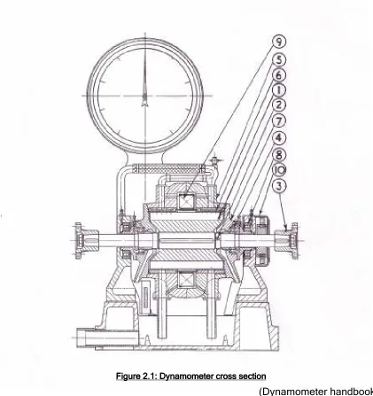
The machine consists of an absorption unit called the stator which is carried upon ball bearings so that it is free to swivel when braking occurs. The torque arm is connected to the stator and a weighting scale is positioned so that it measures the force exerted by the stator in attempting to rotate. The torque is the force indicated by the scales multiplied by the length of the torque arm measured from the center of the dynamometer. The rotor which is inside the stator is coupled to the tested engine and is free to rotate at any speed depending on the dynamometer operating mode.

[image:18.595.93.514.268.715.2]

Figure 2.

Figure 2. Figure 2.

Figure 2.111: Dynamometer cross section1: Dynamometer cross section: Dynamometer cross section : Dynamometer cross section

(19)

(1) Rotor (6) Stator inner rings

(2) Main shaft (7) Stator end cover

(3) Half coupling (8) Stator trunnion bearing (4) Main shaft bearing (9) Field Coil

(5) Stator (10) Governor Generator

For the braking process to occur, the dynamometer is securely bolted to substantial foundation. This assures steady running and eliminates most of the vibrations generated by the system (dynamometer handbook).

• Cooling system

The eddy current induced in the inner rings of the stator generates heat while the rotor is moving. The heat caused by the eddy current is cooled with water. Water is admitted to the gap between the rotor and stator and emerges through ports at the bottom of the machine (dynamometer handbook). To assure that temperature control is maintained while the system is running, a water pressure sensor switch has been included within the water cooling system. If failure of water supply occurs, the switch opens the protective circuit and thus shuts down the engine. In order for the inner rings to be cooled efficiently the quantity of water supplied to the dynamometer must be sufficient. Therefore, if the water pressure falls below an adjustable pre-set value the water pressure switch will open.

• Measuring the speed

(20)

One of the main characteristics of tacho generators is to output a voltage that is proportional in amplitude and frequency to the rotational speed. The generator is mounted onto the dynamometer shaft. The output of the generator is approximately 2 volts per 100 r.p.m (dynamometer handbook).

.

• The control desk

[image:20.595.236.376.359.575.2]

This control unit has been built within a sheet steel control desk and is free to move at any distance from the dynamometer. This control unit is designed to operate from a single phase AC source. Located on the top of the control desk is the r.p.m indicating dial connected to the tachometer.

Figure 2.2: Control desk of the dynamometer Figure 2.2: Control desk of the dynamometerFigure 2.2: Control desk of the dynamometer Figure 2.2: Control desk of the dynamometer

• Governed and Ungoverned option

(21)

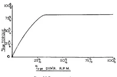
desired torque/speed dynamometer characteristic under specific running conditions. When the system is running under “governed” conditions, it provides a constant D.C. current which flows through the coil irrespective to any speed rise of the rotor. With this arrangement the dynamometer has a natural torque/speed characteristic as depicted in figure 2.3.

[image:21.595.119.514.233.495.2]

Figure 2.3: Figure 2.3: Figure 2.3:

Figure 2.3: TTTTorque vs. speedorque vs. speedorque vs. speedorque vs. speed curve curve curve curve

(Dynamometer handbook)

(22)

2.2 Electromagnetic principle

Understanding the mechanism involved within the Heenan-dynamometer requires an understanding of the electromagnetic concepts applied to it. A permanent magnet has a natural magnetic field around it, as depicted in figure 2.4. The magnetic field, or field of influence, can be virtually represented by lines of magnetic flux. Those lines are completely closed curved, have a definite direction and are perfectly elastic (Sharma 2005).

Similarly, electromagnets generate a magnetic field with the same properties; however the latter relies on electric current to generate its field of influence.

Figure 2.4: Magnetic field of a permanent magnet Figure 2.4: Magnetic field of a permanent magnet Figure 2.4: Magnetic field of a permanent magnet Figure 2.4: Magnetic field of a permanent magnet

(Source: http//www.geocities.com)

2.2.1 T 2.2.1 T 2.2.1 T

2.2.1 The magnetic field of a current carrying conductor he magnetic field of a current carrying conductor he magnetic field of a current carrying conductor he magnetic field of a current carrying conductor

(23)

As represented in the figure 2.5, the surrounding field is generally represented by concentric circles lying on a plane perpendicular to the conductor.

Figure 2.5: Magnetic field of a current carrying conductor Figure 2.5: Magnetic field of a current carrying conductor Figure 2.5: Magnetic field of a current carrying conductor Figure 2.5: Magnetic field of a current carrying conductor

(Source: http//www. bibleocean.com)

When two direct currents flowing in the same direction are applied to two parallel conductors close to each other, the flux lines combine, and the two conductors attract each other.

[image:23.595.213.377.562.680.2]

However, when two direct currents flowing in the opposite direction are applied to two parallel conductors close to each other, the flux lines are crowded together in the space between the conductor, and the two conductors repel each other. Thus, when a direct current is applied to a solenoid, a magnetic field similar to the permanent magnet magnetic field is generated as illustrated in figure 2.6.

Figure 2.6: Mag Figure 2.6: Mag Figure 2.6: Mag

Figure 2.6: Magnetic field around a solenoid netic field around a solenoid netic field around a solenoid netic field around a solenoid

(24)

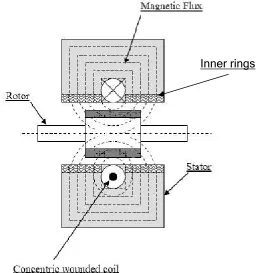
The direction of flux line is defined by the right hand thumb rule. When the solenoid is held in the right hand so that the fingers points in the direction of the current flow, the thumb points to the north pole of the solenoid. Similarly, when a direct current runs trough the dynamometer coil, a magnetic field is generated. Figure 2.7 represents the steady magnetic field generated by the concentric coil within the stator of the dynamometer.

Figure 2.7: Magnetic field generated within the dynamometer Figure 2.7: Magnetic field generated within the dynamometer Figure 2.7: Magnetic field generated within the dynamometer Figure 2.7: Magnetic field generated within the dynamometer

When current is flowing through the dynamometer’s coil a magnetomotive force (m.m.f) also called a magnetic potential is created. The m.m.f produces the primary magnetic fields of the system and is given by equation (2.1). The m.m.f is proportional to the current and the number of turn of the solenoid.

N I f m

m. . = . (Ampere-turns) (2.1)

[image:24.595.192.449.228.501.2]

(25)

In the dynamometer system the number of turns is fixed, consequently the magneto motive force will only be proportional to the amount of current through the solenoid.

2.2.2 Eddy current 2.2.2 Eddy current 2.2.2 Eddy current 2.2.2 Eddy current

When a moving magnetic field intersects a conductor, or a moving conductor intersects a magnetic field, current is induced. The relative motion causes a circulating flow of electrons within the conductor. These currents, also called eddy currents or Foucault currents, create electromagnets with magnetic fields that oppose the change in the primary magnetic field.

The m.m.f generated by these eddy currents is proportional to the strength of the original magnetic field, and also to the speed at which the magnetic field or the conductor is moving. These eddy currents are induced to the inner rings of the stator (see figure 2.7) when the rotor starts spinning within the magnetic field. The rotor is of high permeability steel and makes with the stator the magnetic circuit of the system. Because of this property, the flux lines are uniformly concentrated at the rotor pole tips to take full advantage of the available area. As a result, the density of the magnetic flux is not the same all around the rotor. Figure 2.8 illustrates the rotor pole tips and the concentration of the magnetic flux due to the magnetic property of the rotor.

The flux density is a vector quantity, and its magnitude is given by equation (2.2). In the SI system the unit of the magnetic flux density is Weber per meter square.

A

B=Φ (Wb/m2) (2.2)

(26)

Flux line

Figure 2.8 Figure 2.8Figure 2.8

Figure 2.8: : : : Magnetic flux density through the rotorMagnetic flux density through the rotorMagnetic flux density through the rotorMagnetic flux density through the rotor

Because of the steady nature of the magnetic field, the rotor will not be affected by any change of magnetic flux density. Therefore no current will be induced on the rotor. However, while the rotor is moving, the inner rings of the stator are subject to a change in magnetic field density.

According to Faraday’s law, whenever there is a relative motion between a conductor and a magnetic field, an electromotive force is induced in the conductor and is proportional to the rate of change at which the field is cut (Sharma 2005). In this case, the inner rings are held stationary and they are subject to varying magnetic fields produced by the rotation of the slotted rotor within the primary magnetic field. These electromotive forces are localized with the inner rings and generate eddy currents due to the resistive nature of the material. Fleming’s Right hand rule can be used to define the direction of the induced electromotive force.

However, in accordance to Lenz’s law, represented by equation (2.3), the eddy currents will always tend to oppose the change in field inducing it.

t N emf

∆ ∆ −

= φ (2.3)

Where N is the number of turn and

t ∆ ∆φ

(27)

2.2.3 El 2.2.3 El 2.2.3 El

2.2.3 Electromagnetic braking effect ectromagnetic braking effect ectromagnetic braking effect ectromagnetic braking effect

The magnetic fields created by the induced eddy current are called the secondary magnetic fields and they attempt to cancel the magnetic field causing it. This phenomenon generates new forces within the dynamometer. One force which acts upon the stator and another force which opposes the first acts upon the rotor, and thus decelerate its motion.

The force acting upon the stator forces it to rotate in the same direction as the rotation of the rotor. The absorption unit is securely bolted to a substantial foundation but is able to swivel clockwise or anti-clockwise depending on the force acting upon it. This tendency to follow the rotor rotation is counteracted by means of a lever arm connected to a sensitive torque measuring apparatus. When the stator swivels, the force applied to it is transferred to the measuring apparatus.

(28)

CHAPTER 3 – RECTIFICATION

The actual dynamometer rectifier is obsolete and uses valve rectifier technology. To update the system with new power electronics, it is convenient for the University of Southern Queensland to change the valve rectifier with solid state devices. This chapter includes an overview of rectifier using solid state devices and demonstrates by means of experiment the basic principles for controlled rectification.

3.1 The power diode or rectifier diode

A diode is a two terminal device that allows an electric current to flow in one direction but essentially blocks it in the opposite direction. The diode circuit symbol is represented in figure 3.1. A semiconductor diode consists of a PN junction and the two terminals are called the anode and the cathode. Current flows from anode to cathode within the diode as shown by the arrow of the circuit symbol.

Figure 3.1: Diode circuit symbol Figure 3.1: Diode circuit symbol Figure 3.1: Diode circuit symbol Figure 3.1: Diode circuit symbol

(29)

[image:29.595.202.395.138.286.2]

Figure 3.2: Idealised Figure 3.2: Idealised Figure 3.2: Idealised

Figure 3.2: Idealised diode characteristicdiode characteristicdiode characteristicdiode characteristic

3.2

3.2 The Thyri

The Thyri

The Thyristor or Silicon C

stor or Silicon C

stor or Silicon Controlled

ontrolled R

ontrolled

R

Rectifier

ectifier

ectifier (SCR)

(SCR)

A thyristor is a semiconductor device that has the same characteristics as the diode. Thyristors are often called silicon controlled rectifiers and compare to the diode the thyristor is a three terminal device. The main terminals of the thyristor are the anode and the cathode. The third terminal is referred as a gate. Figure 3.3 illustrate the thyristor circuit symbol.

Figure 3.3: Thyristor circuit symbol Figure 3.3: Thyristor circuit symbolFigure 3.3: Thyristor circuit symbol Figure 3.3: Thyristor circuit symbol

In the case that the thyristor is connected in series with a load through an AC source, no current flows through the circuit until the thyristor as received a triggering signal at the gate terminal.

Anode Cathode

(30)

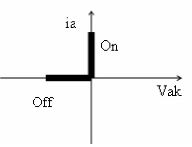
When the pulse is received it triggers the thyristor and allows current to flow from anode to cathode. Figure 3.4 illustrate thyristor idealised characteristic.

Figure 3.4: Typical thyristor characteristic Figure 3.4: Typical thyristor characteristic Figure 3.4: Typical thyristor characteristic Figure 3.4: Typical thyristor characteristic

Once triggered the thyristor continues to allow current to flow through the circuit during the first half cycle of the supply. During the next half cycle the thyristor does not conduct because it is reversed-biased.

However, to conduct after been triggered, the current through the thyristor has to be higher than the latching current and last for a certain period of time. To turn off, the anode current is reduced below the holding current.

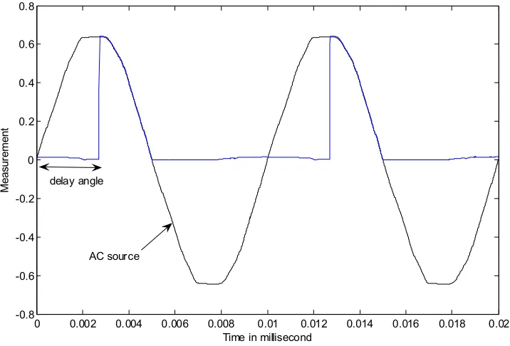
The most important characteristic of silicon controlled rectifiers is that conduction can be delayed in each half cycle, to achieve a variable output voltage. The triggering pulse causing the conduction of the thyristor to be delayed is generated by the firing module.

(31)

0 0.002 0.004 0.006 0.008 0.01 0.012 0.014 0.016 0.018 0.02 -0.8 -0.6 -0.4 -0.2 0 0.2 0.4 0.6 0.8 M e a su re m e n t

Time in millisecond delay angle

AC source

Figure 3.5 illustrates the delay of conduction also called the delay angle.

[image:31.595.125.483.155.398.2]

Figure 3.5: Half controlled half wave rectifier Figure 3.5: Half controlled half wave rectifier Figure 3.5: Half controlled half wave rectifier Figure 3.5: Half controlled half wave rectifier

• The firing module

The firing circuit must be designed so that it will only give a firing pulse during the time that the thyristor is forward biased. If the gate pulse is applied at the beginning of the half-cycle, the complete half-cycle will be applied to the load. If the gate pulse is applied anywhere else during the half-cycle, only a portion of the half-cycle is applied to the load. It is therefore possible to control the load voltage by controlling the gate pulse position.

(32)

As a result, the gate terminal receives a pulse generated by the firing module that will trigger the solid state switch at a specific delay angle.

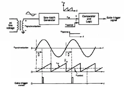
Figure 3.6 represents the block diagram of a triggering module and the waveforms obtain for the triggering process. Basically, a saw tooth generator outputs a saw tooth waveform (Vst) that resets at the zero crossings of the mains supply voltage.

A controllable voltage (Vc) is generated by means of a potentiometer and

compared to Vst. So the output of the voltage comparator (Vp) will be low if the

control voltage is greater than Vst and vice versa. Finally, Vp is fed to a logic circuit

and converted a triggering pulse which is sent to the thyristor gate terminal. (Afhock, 2005).

[image:32.595.98.530.350.663.2]

Figure 3.6: Gate trigger control circuit and waveforms Figure 3.6: Gate trigger control circuit and waveforms Figure 3.6: Gate trigger control circuit and waveforms Figure 3.6: Gate trigger control circuit and waveforms

(33)

3.3 Rectifiers configurations

The coil of the dynamometer requires direct current to generate a steady magnetic field for the braking process to occur. Consequently, conversion of AC to DC must be achieved.

3.3.1 Half and full wave rectification 3.3.1 Half and full wave rectification 3.3.1 Half and full wave rectification 3.3.1 Half and full wave rectification

The process of converting AC to DC is called rectification. The majority of the DC loads respond to the mean value of a periodic wave form. To obtain the mean value of a periodic signal, the integral of the signal during one period is divided by the period in which it occurs. The waveform obtained from the mains is similar to a sinusoidal signal represented in figure 3.7. When using the mean value formula on a sinusoidal signal, the result will be zero as the net area for one period is equal to zero.

Figure 3.7: Sinusoidal wave form Figure 3.7: Sinusoidal wave form Figure 3.7: Sinusoidal wave form Figure 3.7: Sinusoidal wave form

Nevertheless, by means of solid state technology it is possible to change the form of the input signal and obtain an applicable mean value of the supplied voltage for the device to operate in DC mode. There are two main manipulations that can be achieved when rectifying a sinusoidal signal. The half wave rectification or the full wave rectification.

• Half wave rectification

(34)

In half wave rectification the positive or negative half of the AC wave is passed easily while the other half is blocked, depending on the polarity of the rectifier. Figure 3.8 demonstrates half wave rectification of a sinusoidal signal.

Figure 3.8: Half wave rectification Figure 3.8: Half wave rectification Figure 3.8: Half wave rectification Figure 3.8: Half wave rectification

The simplest form of rectifier circuit is a diode connected in series with the ac input. During the positive half cycle of the input voltage the current represented in figure 3.9 flows through the load resistor. The diode offers a very low resistance and hence the voltage drop across it is very small. Thus the voltage appearing across the load is practically the same as the input voltage at every instant. During the negative half cycle of the input voltage the diode is reverse biased. Practically no current flows through the circuit and almost no voltage is developed across the resistor.

So, when the input voltage is going through its positive half cycle, the output voltage is almost the same as the input voltage and during the negative half cycle no voltage is available across the load. This explains the unidirectional pulsating DC waveform obtained for half rectification in figure 3.8.

(35)

This rectifier configuration is classified as uncontrolled rectification. In half wave rectification the AC source only works to supply power to the load once every half-cycle, meaning that much of its capacity is unused. However, half-wave rectification is the simple way to reduce power to a resistive load.

The Average voltage or the DC content of the voltage across the load is given by:

[

]

π

ω

π

ω

ϖ

ω

π

π π π π peak peak av av peak av peak av peak av

I

R

V

R

V

I

V

t

V

t

d

t

d

t

V

=

−

=













+

=

∫

.

cos

2

)

(

.

0

)

(

sin

.

2

1

0 2 0

• Full wave rectification

Figure 3.10 illustrates full wave rectification of the same sinusoidal signal. The negative or positive portions of the alternating signal are reversed and thus produce an entirely positive or negative signal waveform depending on how the diodes are connected.

(36)

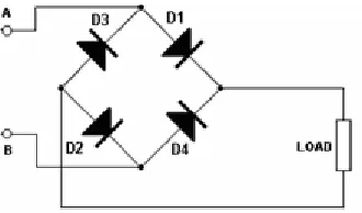
For greater efficiency, it is more convenient to use both halves of the incoming AC source. A rectifier that converts both half-cycles of an AC voltage waveform to a series of voltage pulses of the same polarity is called a full wave rectifier. To obtain full rectification, a different rectifier circuit configuration must be used. Full wave rectifier uses a four diode bridge connection which is illustrated in figure 3.11. If the AC is centre-tapped, then the diodes are arranged anode-to-anode or cathode-to-cathode to form a full-wave rectifier.

Figure 3.11: Diode Bridge rectifier Figure 3.11: Diode Bridge rectifier Figure 3.11: Diode Bridge rectifier Figure 3.11: Diode Bridge rectifier

For the diode bridge circuit, the input signal is a sinusoidal voltage source. During the first half cycle, the voltage is positive. Consequently at point A the voltage is positive and at point B the voltage is negative.

The Anode of D1 and D2 is positive and the cathode of D1 and D4 is negative. During the first half cycle, A is positive and B is negative, consequently diode D1 and D2 are forward biased and current flows from the source through D1, the load and D2 and back into the source.

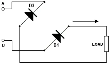
[image:36.595.219.384.259.356.2]

Figure 3.12: Flow of curre Figure 3.12: Flow of curre Figure 3.12: Flow of curre

(37)

During the next half cycle, the voltage at point A is negative and the one at point B is positive. As a result D4 and D3 are forward biased because their anode voltage is positive and their cathode voltage is negative. During this period of time the current will flow around the circuit as shown in figure 3.13, again flowing in the same direction through the load and producing another positive pulse of voltage.

[image:37.595.218.408.227.334.2]

Figure 3.13: Flow of current during negative cycle Figure 3.13: Flow of current during negative cycle Figure 3.13: Flow of current during negative cycle Figure 3.13: Flow of current during negative cycle

The process of full wave rectification is illustrated in figure 3.10. When bridge rectifiers use only diodes they are said to be uncontrolled. So as long as the AC input does not vary it is not possible to adjust their D.C output. However, combining diodes and thyristor within a bridge configuration leads to phase controlled rectification.

The Average voltage or the DC content of the voltage across the load is given by:

(38)

SCR1

D2 D1

3.3.2 3.3.2 3.3.2

3.3.2 Half Half Half and fully controlled rectifier Half and fully controlled rectifier and fully controlled rectifier and fully controlled rectifier

By using different combinations of diode and thyristor it is possible to obtain different classes of rectifiers. Mainly because of the thyristor characteristic of being able to be phased controlled, rectifier are said to be fully controlled when using four thyristors within a bridge configuration.

The fully controlled bridge is usually used when it is necessary to regenerate power form the load. The most widely used rectifier configuration is the half-controlled bridge illustrated in figure 3.14. The main advantage of using half controlled rectification is to provide the load an adjustable D.C output voltage that varies with respect to the delay angle.

For most of the applications using half controlled rectifiers, the control is only possible during positive output voltage from the mains, and no control is possible when the mains cycles are negative.

[image:38.595.208.405.428.528.2]

Figure 3.14: Half controlled bridge rectifier (SCR serie) Figure 3.14: Half controlled bridge rectifier (SCR serie) Figure 3.14: Half controlled bridge rectifier (SCR serie) Figure 3.14: Half controlled bridge rectifier (SCR serie)

3.4 Testing on phase controlled rectifier

A series of tests on a half controlled rectifier provided by the engineering faculty have been conducted in order to understand the process of rectification using this configuration. In the following experiments two different rectifier configurations

SCR2

(39)

D1 SCR1

SCR2

D2

Most of the power electronic applications operate at a relative high voltage and in such cases the voltage drop across the SCR tends to be irrelevant for such application. So, most of the time, the conduction voltage drop across the device is assumed to be zero for circuit analysis. Similarly, it is also valid to assume that the current through the thyristor is zero when it is not conducting.

3.4.1 3.4.1 3.4.1

3.4.1 The half controlled bridge rectifierThe half controlled bridge rectifierThe half controlled bridge rectifier The half controlled bridge rectifier

There are two single phase half controlled rectifier configurations and both operate in a same manner when connected to a resistive load. Figure 3.14 illustrate thyristors in series configuration and figure 3.15 shows the parallel thyristors’ configuration.

Figure 3.15: Half controlled bridge rectifier (SCR parallel) Figure 3.15: Half controlled bridge rectifier (SCR parallel) Figure 3.15: Half controlled bridge rectifier (SCR parallel) Figure 3.15: Half controlled bridge rectifier (SCR parallel)

The delay angle has been fixed to a particular value and the circuit is operating at steady state. During the first half cycle of the AC source, the voltage at point A is positive with respect to B. So, the load current flows only if SCR2 is triggered.

SCR2 is then turned off when the source voltage becomes negative. During this

cycle, B is positive with respect to A, so that SCR1 and D2 conduct the load current

when SCR1 is triggered. However, during the laps of time when SCR1 has not

(40)

0 0.002 0.004 0.006 0.008 0.01 0.012 0.014 0.016 0.018 0.02 -0.8 -0.6 -0.4 -0.2 0 0.2 0.4 0.6 0.8

RESISTIVE AND INDUCTIVE LOAD

M e a s u re m e n ts

Time in millisecond Main voltage

Load current Rectified voltage

This inductive current has two circuits where it can flow, one made by the SCR2,

the source and D1 and a second, made by SCR1 and D1. Because of the low

impedance of the second circuit, the current continue to flow through SCR1 and D1

while the voltage is negative.

The back e.m.f from the inductive load drives current through the bridge without containing any of the reverse supply voltage. During this time interval the load current decays exponentially. Thyristor SCR1 is then triggered in the next half

cycle and the cycle repeats. Figure 3.16 illustrates the output of a half controlled bridge rectifier connected to an inductive load.

[image:40.595.74.522.319.633.2]

(41)

This half control rectifier configuration is good when the load is not too inductive and with a time constant much lower than one half cycle of the supply. On a contrary, if the load is highly inductive with a time constant greater than one half-cycle of the supply, it will become more difficult to turn off the load current just by not sending any pulse to the gate.

If the trigger pulses are removed after that a thyristor has been triggered, this thyristor will continue to conduct as usual for the rest of the half cycle of the supply. Then, the other thyristor will not turn on because no triggering pulse will be sent to assure conduction. The circuit will continue to operate indefinitely with the first triggered thyristor conducting on complete alternate half cycle and acting as a flywheel diode on the other half cycles. In this case, the only way to interrupt this cycle will be to stop the mains supply. Nevertheless, to ensure that the circuit operates satisfactorily a free wheeling diode can be added in parallel to the load. Consequently, at the end of each half cycle of the supply the load current is transferred directly to this diode. The free wheeling diode ensures that there is no risk that a thyristor will continue to conduct over another half cycle. (ed. Mullard 1970).

The average output voltage of the bridge as a function of firing angle:

(42)

The RMS load current during α < wt < π :

]

[

)

sin(

)

(

)

(

tan

1

]

[

)

sin(

)

(

1 2 τ α π τ α ϖ

β

π

τ

β

ω

τ

β

ω

− − − − −

×

+

−

×

=

+

×

=

×

+

−

×

=

e

A

Z

V

i

and

R

L

R

Z

where

e

A

t

Z

V

t

i

peak load t peak load

TheRMS load current during π < wt < π + α :

]

[

)

(

)

(

τ π ϖ

π

ω

− −

+

=

t load

load

t

i

When the load current is repetitive

(43)

0 0.002 0.004 0.006 0.008 0.01 0.012 0.014 0.016 0.018 0.02 -0.8 -0.6 -0.4 -0.2 0 0.2 0.4 0.6 0.8

RESISTIVE AND INDUCTIVE LOAD

M e a s u re m e n ts

Time in millisecond

Once A is known, the total RMS value of line current and the RMS value of its fundamental component can be estimated.

3.4.2 Fully controlled half wave rectifier with a free wheeling diode 3.4.2 Fully controlled half wave rectifier with a free wheeling diode 3.4.2 Fully controlled half wave rectifier with a free wheeling diode 3.4.2 Fully controlled half wave rectifier with a free wheeling diode

The operation of this rectifier configuration is very similar to the single diode circuit represented in figure 3.9. The only difference is that this configuration uses a thyristor connected in series with the load and a diode connected in parallel.

[image:43.595.87.512.294.591.2]

Figure 3.17: fully controlled half wave rectifier output Figure 3.17: fully controlled half wave rectifier output Figure 3.17: fully controlled half wave rectifier output Figure 3.17: fully controlled half wave rectifier output

(44)

As explained earlier, when the thyristor is triggered in the forward-bias state, it starts conducting and the positive source keeps the device in conduction until the source voltage becomes negative. At that instant, the current through the circuit is not zero because there is some energy that has been stored in the inductor.

(45)

CHAPTER 4 – TEST AND DESIGN

The updated half wave rectifier has to be tested on the dynamometer. Subsequently, tests will be implemented in order to localise where the upgraded rectifier will be connected.

4.1 Input and output location

Originally, the protective circuit of the initial circuit was supposed to be reused with the upgraded rectifier circuit. However, this task was requiring meticulous investigations and thus more time. Therefore, it was more convenient to re-design the whole unit control and keep the valve circuit intact. As a result, the entire valve system was disconnected so that if the upgraded system fails to operate, the initial electronic unit will still be able to operate the plant. The first approach was to determine the input and output connections of the circuit.

[image:45.595.205.432.461.683.2]

Figure 4.1: External wiring connection of the dynamometer Figure 4.1: External wiring connection of the dynamometer Figure 4.1: External wiring connection of the dynamometer Figure 4.1: External wiring connection of the dynamometer

(46)

Figure 4.1 illustrates the connections between the dynamometer bed plate connector block and the electronic input panel. As depicted, none of the dynamometer bed plate connections are well defined. However, it can be seen that the dynamometer is connected to the electronic circuit via six input or output connections.

The dynamometer must be protected against over heating. In the cooling system located on the dynamometer side, is embedded a water pressure switch which senses the water pressure. If the water pressure is not sufficient the switch opens a protective circuit which shuts down the engine coupled to the dynamometer. Consequently, there must be a signal from the dynamometer to indicate low water pressure level.

Similarly, the dynamometer has to be protected against over speeding. As explained in the handbook, if the dynamometer speed rises above a preset value the system will also shuts down automatically. Consequently, an output signal from the tacho generator which is located on the dynamometer side must be fed to the control unit to detect when the engine speed goes above a speed limit.

Finally, the dynamometer field coil has to be roused to generate the primary magnetic field for braking process to occur. So, there must be an input signal from the circuit that regulates the amount of current going through the coil.

4.2 Preliminary tests

(47)

The information contained within the handbook does not define any of these connections; subsequently assumptions were made before implementing tests on the dynamometer.

At first, connection C1 and C2 were assumed to refer to the coil connection and therefore enables a signal to go from the electronic circuit to the field coil. Then, it was assumed that connection W1 and W2 were assumed to refer to the water pressure switch located within the dynamometer. And finally, connection A1 and A2 were assumed to be the analogue signal generated by the tacho generator to prevent the engine to over speed.

Connection IG.1, IG.2, and IG.3 are defined as the engine ignition connection and are used to safeguard the engine in case of overspending, or failure of water or electricity supplies. The main power supply is defined by the L and N connections to operate the whole system.

To verify the assumptions about connections C1, C2, A2, A1, W2, W1, a series of tests were implemented on the dynamometer bed plate connections.

• Test at terminals C1and C2

The input signal of the excited coil must be a rectified version of the main source voltage. The best approach to ensure that C1 and C2 are the dynamometer coil input connections a digital oscilloscope was connected across them. Figure 4.2 illustrates the signal obtain across these connections.

(48)

- 0.0 2 5 - 0.0 2 - 0 .0 1 5 - 0 .0 1 - 0 .0 05 0 0 .00 5 0 .0 1 0. 01 5 0.0 2 0. 025 - 0 .1

0 0 .1 0 .2 0 .3 0 .4 0 .5 0 .6 0 .7

O utpu t fr o m c on n ectio n C 1 a n d C 2

re ct if ie d V ol ta ge w a v e fo rm

[image:48.595.64.521.105.360.2]

Ti me i n m illise co n d Figure 4.2: Signal obta Figure 4.2: Signal obtaFigure 4.2: Signal obta

Figure 4.2: Signal obtained across connection C1 and C2ined across connection C1 and C2ined across connection C1 and C2ined across connection C1 and C2

• Test at terminals W1 and W2

As explained before, W1 and W2 are assumed to be the water pressure switch connection of the protective circuit. Consequently, these connections must be connected at both ends of the switch represented in figure 5.1.

A perfect switch, by definition, will have 0 Ω when closed and it will have infinite resistance when opened. To check the resistance between these two connections, an ammeter was connected across them.

(49)

- 3 - 2 - 1 0 1 2 3

x 10- 3

- 0 .1 - 0 .0 8 - 0 .0 6 - 0 .0 4 - 0 .0 2 0 0 . 02 0 . 04 0 . 06 0 . 08 0 . 1

O utp u t f r o m c on n e c t io n A 1 a n d A 2

T a ch o m e te r o u tp u t v o lt a g e

T i m e in m i llis e c o n d • Test at terminals A1 and A2

The system uses an analogue tachometer mounted on the dynamometer shaft. The device generates an output voltage that is proportional to the rotational speed.

To prove that A1 and A2 are the tachometer outputs, a digital oscilloscope was connected across these connections while the system was running. As assumed, when the speed was increased or decreased the signal amplitude and frequencies were changing with respect to the engine speed. Figure 4.3 shows the output of the tacho generator at a certain speed.

[image:49.595.75.488.325.580.2]

Figure 4.3: Figure 4.3: Figure 4.3:

Figure 4.3: Signal obtain Signal obtain Signal obtain Signal obtain across across across connection across connection connection connection AA1 and AA1 and 1 and A1 and AAA222 2

To confirm that the voltage was changing with respect to speed, the proportionality between speed and amplitude was also checked. When the system was running, the voltage RMS and speed reading were proceed and stored in table 4.1.

(50)

Tachometer linearity speed vs voltage

0 500 1000 1500 2000 2500 3000 3500

20.9 29.6 38.9 49.6 58.8

[image:50.595.168.470.364.588.2]

Voltage rms s p e e d r p m

Table 4.1: Tacho generator output voltage at a certain speed Table 4.1: Tacho generator output voltage at a certain speed Table 4.1: Tacho generator output voltage at a certain speed Table 4.1: Tacho generator output voltage at a certain speed

The following figure illustrates the proportional relationship between speed and the voltage.

Figure 4.4: Linearity between the output voltage and speed Figure 4.4: Linearity between the output voltage and speed Figure 4.4: Linearity between the output voltage and speed Figure 4.4: Linearity between the output voltage and speed Speed RPM VOLTAGE RMS

1000 20.9

1500 29.6

2000 38.9

2500 49.6

3000 58.8

(51)

CHAPTER 5 – PROTECTIVE SYSTEM

Protection of the plant while it is operating is essential. The whole plant has to be protected against over speeding and overheating. At the same time, the user must be safe and has to be protected against any independent emergency. This chapter explains the use of a protective circuit and briefly describes the protective system used with the valve rectifier. Following that, it gives a description of the selected devices used for protection.

5.1 The existing protection system

The circuit depicted in figure 5.1 represents the actual protective circuit that safeguards the engine and the dynamometer in the event of water failure, over speeding or failure of the power supply.

Figure 5.1: Existing protective circuit Figure 5.1: Existing protective circuit Figure 5.1: Existing protective circuit Figure 5.1: Existing protective circuit

(52)

5.1.1 The water pressure a 5.1.1 The water pressure a5.1.1 The water pressure a

5.1.1 The water pressure and ignition switchesnd ignition switchesnd ignition switchesnd ignition switches

• The water pressure switch

Cooling the dynamometer inner rings is essential to safeguard the dynamometer because considerable damage would be done if the instrument overheated. The heat generated by the induced current would melt the stator inner rings if they are not cooled properly.

As explained in the dynamometer handbook, each brake power absorbed generates 42.4 B.Th.U per minute, nearly all of which passes into the cooling water. Consequently, the water pressure must be sufficient to ensure the temperature of the stator inner rings does not rise above 140 degrees Celsius.

To sense the water pressure in the cooling system, a specific protective device is used. It is referred in to the handbook as the water pressure switch. The switch is embedded within the dynamometer cooling system and is connected to the electronic unit by means of the connections W1 and W2. When water is running through the dynamometer with enough pressure, the water pressure switch closes a protective circuit so that the system is safe to run. On the contrary, if the water pressure is not sufficient to cool the inner rings, the switch opens the protective circuit so that the system is shut down or cannot start.

• The ignition switch

(53)

5.1.2 The connections of the coil ignition engin 5.1.2 The connections of the coil ignition engin5.1.2 The connections of the coil ignition engin 5.1.2 The connections of the coil ignition engineeee

IG.1, IG.2 and IG.3 are the three terminals from the electronic input panel connected with the engine ignition system. The Low Tension connections of the coil ignition engine are connected in series with terminal IG.1, IG.2 and IG.3. These terminals are connected to the second ‘change-over contact’ of a double pole double throw relay as depicted in figure 5.2.

[image:53.595.226.395.366.485.2]

To stop the engine when a fault occurs, the change over contact has to be on IG.1 and IG.2. For the engine to start, IG.2 and IG.3 must be connected. The Double Pole Change Over (D.P.C.O) relay has two rows of change-over terminals and is actuated by a single coil.

Figure 5.2: Double Pole Double Throw relay (DPDT) Figure 5.2: Double Pole Double Throw relay (DPDT)Figure 5.2: Double Pole Double Throw relay (DPDT) Figure 5.2: Double Pole Double Throw relay (DPDT)

(Handbook, 1881)

5.1.3 Resetting the DPCO relay 5.1.3 Resetting the DPCO relay 5.1.3 Resetting the DPCO relay 5.1.3 Resetting the DPCO relay

(54)

As a result, the engine is ready to be started and the whole system is safe to operate. For the engine to start, the entire set of switches that constitute the protection system have to be closed. If any of the switches open while the system operates the engine is turned off automatically. For example, if the water pressure is insufficient, the water pressure switch will open. Consequently, the coil of the relay will be de- energized and the relay will return to its initial state where IG.2 is connected to IG.1.

5.1.3 Over speed control 5.1.3 Over speed control 5.1.3 Over speed control 5.1.3 Over speed control

The function of the first relay RL1, represented in figure 5.2, is to stop the prime mover if the load generated by the dynamometer fails. When the load fails it is commonly due to either a failure of the main supply or a fault occurring within the excitation unit. If a sudden failure of the load occurs, the speed of the engine will rise so quickly that considerable damages would occur to the prime mover.

In figure 5.1, valve V8 is biased off by adjusting the potentiometer P3. The position of P3 determines the speed at which the plant should shut down. V8 will remain biased off until the rectified signal from the tacho generator exceeds the bias condition. In the case that the rectified D.C signal exceeds the over speed cut out adjustor limit, V8 will allow current to pass and will energised the coil of RL1. As a result, Relay one open the protective circuit and de-energises Relay two (RL2) which closes contacts IG.1 and IG2(Dynamometer handbook).

5.2 Upgraded protection system

(55)

The circuit guarantees that the engine stops automatically in the event of insufficient water pressure, over speeding or a fault occurring in the excitation unit. For design simplicity and convenience, the water pressure sensor has been re-used.

5.2.2 5.2.25.2.2

5.2.2 Over speeding protection device Over speeding protection device Over speeding protection device Over speeding protection device

As explained earlier, the circuit must prevent over speeding for engine protection. When the speed of the dynamometer shaft rises above a preset value, the prime mover must stop. The most suitable device for this operation is the Multifunction Voltage Relay also called the M3MVR. As a result, the section of the initial protective circuit represented in figure 5.3 is replaced by using only this device.

Figure 5.3: Over speed protection used with initial design Figure 5.3: Over speed protection used with initial design Figure 5.3: Over speed protection used with initial design Figure 5.3: Over speed protection used with initial design

(Dynamometer handbook)

(56)

[image:56.595.210.394.115.254.2]

Figure 5.

Figure 5.Figure 5.

Figure 5.4444: : : : M3MVR and front panel M3MVR and front panel M3MVR and front panel M3MVR and front panel

(Source: http://www.broycecontrol.com)

For this application, the M3MVR is used to track if the voltage output from the tacho generator goes above a preset voltage. As soon as the M3MVR receives an analogue signal with a peak value above the limit, the internal switch opens and thus opens the protective circuit, stopping the engine.

When the relay has triggered it can be reset by either momentarily removing the power supply or turning the latch switch to the off position.

(57)

[image:57.595.195.393.121.260.2]

Figure 5.5: Timing diagram for over voltage monitoring Figure 5.5: Timing diagram for over voltage monitoring Figure 5.5: Timing diagram for over voltage monitoring Figure 5.5: Timing diagram for over voltage monitoring

(Source: http://www.broycecontrol.com)

If the relay is monitoring close to its tripping point, it might continuously pull in and drop out as the voltage continually passes through the set point. To overcome this problem, an adjustable hysteresis level has been incorporated to the relay. This causes the relay to re-energise at a point which is at either 2% or 10% below the set point level. The choice of hysteresis level can be made using the front mounted switch (see figure 5.4). The M3MVR is able to monitor two different ranges of voltages.

M3MVR technical specifications:

Supply voltage (nominal): 18 – 240 V AC 50/60 Hz Min./max limits : 15 – 265 V AC 48/63 Hz

Power consumption: 3 VA

Output contact ratings: 8 A, 250V AC Input impedance: 10 MΩ

Monitoring ranges:

(58)

Figure 5.6 represents the section of the upgraded protection circuit that will protect the engine against over speeding.

Figure 5.6: M3MVR Figure 5.6: M3MVR Figure 5.6: M3MVR Figure 5.6: M3MVR

5.2.3 Resetting the initial state of the circuit 5.2.3 Resetting the initial state of the circuit 5.2.3 Resetting the initial state of the circuit 5.2.3 Resetting the initial state of the circuit

The most suitable relay