Rainfall prediction using Machine Learning Techniques

International Journal of Innovative Technology and Exploring Engineering (IJITEE) ISSN: 2278-3075, Volume-8 Issue-7, May, 2019



Abstract: Rainfall prediction is very important in several aspects of our economy and can help us preventing serious natural disasters. Some areas in India are economically dependent on rainfall as agriculture is primary occupation of many states. This helps to identify crops patterns and correct management of water resources for the crops. For this, linear and non-linear models are commonly used for seasonal rainfall prediction. Few algorithms used for rainfall prediction are CART, Genetic Algorithms and SVM, these are computer aided rule-based algorithms. In this paper, we performed qualitative analysis using few classification algorithms like Support vector machines(SVM), Artificial Neural Networks, Logistic regression. Dataset used for this classification application is taken from hydrological department of Rajasthan. Overall, we analyze that algorithm which is feasible to be used in order to qualitatively predict rainfall.

Index Terms: Rainfall prediction, Correlation based feature selection, Machine Learning.

I. INTRODUCTION

Weather forecasting is an imperious and demanding task that is carried out by various weather departments from around the world in order to inform the common people such as ourselves about the weather. It is an intricate procedure that encompasses various specialized fields. This specific objective in this domain is complicated due to the nature of taking decisions in an uncertain manner. A diverse group of scientists from all over the world has developed stochastic weather models with the help of Random Number Generator, which can produce an output that resembles the weather data, aiding them to build a huge dataset without any need of manual recording. India is a country that consists of more than a billion people and more than 60% of this population are dependent upon agriculture for a living. the special field of rainfall prediction, which is necessary for all the people. Rainfall prediction plays a vital in preventing causalities caused due to natural disasters. It also helps us to maintain our water resources properly. Highly accurate rainfall prediction is useful in case of heavy rainfall which might cause flood and no rainfall which may cause drought to maintain our water resources. In the country like India,

Revised Manuscript Received on May 08, 2018.

G. Bala Sai Tarun, CSE, Koneru Lakshmaiah Education Foundation, Guntur, India.

J.V. Sriram, CSE, Koneru Lakshmaiah Education Foundation, Guntur, India.

K. SaiRam, CSE, Koneru Lakshmaiah Education Foundation, Guntur, India

K. Teja Sreenivas , Koneru Lakshmaiah Education Foundation, Guntur, India.

M V B T Santhi, , Associate Professor, computer science engineering, KLEF Guntur, India.

where crops are harvested based on the monsoon season. So, having advanced knowledge in prediction is important. Some states are affected by droughts while some with floods. This prediction model can help us to take required precautions to save lives by providing transport and food. To solve this problem, various rainfall predictions methods have been proposed. However, these methods have performance limitations because of wide range of variations in data and amount of data is limited. Many approaches like stochastic method, statistical methods and neural networks have been used. Some of these approaches showed promising results with good performance while others did not provide transparent reasons.

A. RelatedWork:

Weather holds a significant role in our daily life, where we can use weather forecasts in order to avoid future disasters or any other hazardous events. Several techniques were proposed by researchers to aid in such tasks. However, this led to the problem to be broken down into two predictive types: Rainfall events (Binary prediction), and classification of rainfall when it is actually present (light, moderate, and strong rainfall). Thus far, ANN was used in this field and it has opened up many new paths in the prediction of environment-related phenomena (Gardener and Dorling, 1998; Hsiesh and Tang, 1998). Various structures of the auto-regressive moving average (ARMA) models, ANN, and Nearest-Neighbor techniques were used for the prediction of storm rainfall that occurred in areas such as the Sieve River Basin, Italy, between the periods of 1992 to 1996. [4] proposed the practice of using ANNS for the forecast of monthly average in rainfall for an area in India based upon the monsoon type climate. This study case considered eight months per year for the prediction. During these months, there was certainty of a rainfall event to occur. The research was performed using three different types of networks: Feed Forward Back Propagation, Layer Recurrent, and Cascaded Feed Forward Back Propagation. The network that obtained the best results was the Feed Forward Back Propagation. Liu et al [2] suggested a substitute method over the previous model. They explore the practice of using genetic algorithm as a feature selection algorithm and the Naïve Bayes algorithm as a predictive algorithm. The use of genetic algorithms for the selection of inputs makes it possible to simplify the intricacy of the data sets and also improving upon the performance.

Rainfall prediction using Machine Learning

Techniques

Shoba G. and Shobha G [1] analyzed various algorithms such as Adaptive Neuro-Fuzzy Inference System (ANFIS), ARIMA and SLIQ Decision for the forecast of rainfall. R.Sangari and M.Balamurugan [3] related data mining methods such as the K-Nearest Neighbor(KNN), Naïve Bayes, Decision Tree, Neural Networks, and Fuzzy Logic for the use of rainfall prediction. Beltrn-Castro[5] used decomposition and ensemble techniques to rainfall on daily basis. Ensemble Empirical Mode Decomposition (EEMD) is the decomposition technique adopted by Beltrn castro for dividing data into multiple segments. Few scholars like D. Nayak and A. Mahapatra [7] used different machine learning algorithms like MultiLayer Perceptron Neural Network (MLPNN), Back Propagation Algorithm(BPA), Radial Basis Function Network (RBFN), SOM (Self Organization Map) and SVM (Support Vector Machine) to predict rainfall. Their results have shown positive results on favor of back propagation algorithm. In [6] authors used different neural network models to predict rainfall. They have adopted feed forward neural network using back propagation, cascade-forward back propagation NN (CBPN), distributed time delay neural network (DTDNN) and nonlinear autoregressive exogenous network (NARX) and compared which gives best results.

B. Issues in Rainfall:

• The initial issue involved in rainfall classification is

choosing the required sampling recess of

Observation-Forecasting of rainfall, which is dependent upon the sampling interval of input data. For Example, let’s take a yearly data, which is quite a large dataset and thus also provides a good accuracy. When we consider smaller training datasets such as daily or weekly, due to the noise and distortion that follow suit with these datasets, the predictions may not be accurate in the long-term with such fluctuations. A monthly or yearly dataset should most likely be used when trying to accurate predict rainfall as there are less abnormal interferences within the dataset.

• The next main issue is choosing the features or parameter for the rainfall prediction. When you incorporate too many or too few input parameters, it can affect the overall calculation of the entire network. So, the selection parameters that are involved in this task are entirely based upon the region of the prediction which includes its geography, and topography to predict the rainfall of this area. Rainfall parameters can also include characteristics such as wind speed, humidity, and soil temperature. Currently, Researchers are using parameters such as maximum temperature, minimum temperature, relative humidity, and such characteristics in order to predict weekly rainfall. Sometimes, this can prove to be a slightly less accurate technique.

• The final issue that is involved in rainfall prediction is electing the appropriate model for the task. Current researches have plenty of algorithms that are readily available in the data mining field but there isn’t enough evidence for selecting the best algorithm that is suited for the

given problem. However, Data Mining algorithms provide excellent solutions for solving similar problems in literature. The underlying task here is to properly figuring which model is required to solve the problem or which algorithms to combine in order for effective predictions. This is clearly a classification problem and hence disqualifies the use of machine learning such as multinomial regression. Instead, we use classification models such as Neural Networks, Logistic Regression, Naïve Bayes, Decision tree classifiers, and more.

II. THEORY AND EXPERIMENTATION

A. Feature Engineering:

High Dimensional data is tricky for classifications algorithms because of its higher computational costs and the required memory usage. To rectify this, we use two dimensionality reduction techniques which are known as feature reduction and feature selection. Feature extraction and selection methods are used either separately or integrated together in order to improve the performance, estimated accuracy, visualization, and comprehension of knowledge. The advantage in using feature selection is that the importance of any small information is not considered as insignificant but when considering a large pool of information which diverse features, some features may be omitted. While in Feature extraction, the size of the feature space is decreased along with minimal loss of info of the original feature space. Choosing between these two techniques is based solely upon the type and domain of the

specific task.

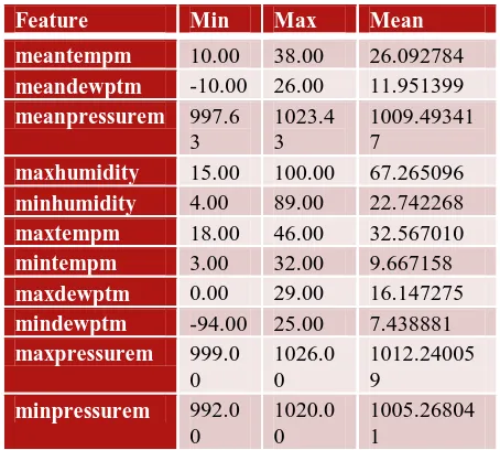
Table 1- Feature Set

Feature Min Max Mean

meantempm 10.00 38.00 26.092784

meandewptm -10.00 26.00 11.951399

meanpressurem 997.6

3

1023.4 3

1009.49341 7

maxhumidity 15.00 100.00 67.265096

minhumidity 4.00 89.00 22.742268

maxtempm 18.00 46.00 32.567010

mintempm 3.00 32.00 9.667158

maxdewptm 0.00 29.00 16.147275

mindewptm -94.00 25.00 7.438881

maxpressurem 999.0

0

1026.0 0

1012.24005 9

minpressurem 992.0

0

1020.0 0

International Journal of Innovative Technology and Exploring Engineering (IJITEE) ISSN: 2278-3075, Volume-8 Issue-7, May, 2019

Table 1 is comprehensive display of set of features and their ranges. We have chosen four attributes- Temperature, Humidity, Dew point temperature, Pressure. To capture complete essence of data we have also considered minimum, maximum and mean of the attributes in our problem thereby giving us a feature set of size 12 including feature ‘precipm’ and excluding ‘mean humidity’.

Feature Extraction: This is a general method where one tries to transform a current input space into a smaller dimensional subspace which can preserve the most pertinent information. Feature extraction can be in used in that sense that it can reduce the complexity and give a much simpler representation of variables in a feature space such as the variables original direct combination. The most commonly used approach for feature extraction is the Principle Component Analysis (PCA), which was introduced by Karl. There have been various iterations and variants of PCA that have been proposed. PCA is basically a method which doesn’t depend on parametric in order to extract the most pertinent information from a redundant set of data. It is a linear transformation of data which minimizes the redundancy and increases the information efficiency. Feature Selection: In this method, a subset from the current data features are selected as input for the progression of a learning algorithm. The subset is chosen based upon the set with the least dimensions that can give the best learning accuracy. Many studies have been performed in order to select the best feature extraction and selection approaches. A few approaches used in feature selection are RELIEF, CMIM, BW-ration, Correlation Coefficient, GA, SVM-REF, Non-Linear PCA, Independent Component Analysis, and Correlation based feature selection.

Advantages of feature selection:

• It is useful in reducing the complexity and dimensionality of a feature space, and limit storage requirements for the subsets.

• It increases the speed of the algorithms due to lower required requirements

• It eradicates redundant and unnecessary data.

• An immediate effect of Feature selection is that it speeds up the run time of learning algorithms.

• The data quality is vastly enhanced

• The accuracy of the resulting model is vastly improved. • Due to the reduction of the features in the dataset, we can use the remaining resources for other tasks or in the next round of data collection.

• The learning algorithm outputs results that are higher in quality and more accurate.

Correlation Based Feature Selection:

In our experimentation we have chosen correlation based feature selection method to find out the best possible subset of features. Correlation-Based Feature Selection (CFS) searches subset of features based upon its degree of

redundancy among the various features. Its evaluation process objective is to find a feature subset which are individually highly related with a class but have a relatively low inter correlation. The significance of the group of features raises with the correlation between the features and a specific class, and also shrinks if there is a growing inter-correlation. CFS is an approach meant to find the best subset of features and it integrated with various search strategies which include forward selection, backward elimination, bi-directional search, best first search, and genetic search.

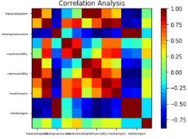
Figure 1-Correalation Analysis

ForFeatureset('meantempm'-0,'meandewptm'-1,'meanpressu rem-2','maxhumidity-3','minhumidity'-4,'maxtempm'-5,'min tempm'-6,'maxdewptm'-7,'mindewptm-8','maxpressurem'-9, 'minpressurem'-10,'pr-ecipm'-11) Figure 1 is correlation analysis representing correlation between different features. Cell(0,0)-corr(‘meantempm', ‘meantempm')

Cell(0,11)-corr(‘meantempm', 'precipm')

Sequential Forward Selection is a simple greedy search algorithm, which is meant for dataset that have a small number of features. This algorithm possesses one drawback; it is unable to remove a feature once it becomes redundant in nature with the addition of other features. Sequential Backward Selection is quite opposite of the Sequential Forward Selection. For SBE, it is best to use it on a large subset of features. The drawback associated with this method is that, it is unable to reconsider the expediency of a feature after it has been removed. Plus-L Minus-R Selection is a generalization of these two approaches which tackles the shortcomings of the above two mentioned approaches.

B. Artificial Neural Networks:

The main advantage of Neural Networks is its ability to display non-linearity existence between the input and output variables.

Figure A.1 : Neural Network

Major concerns with neural networks

1.Number of Hidden Layers and Nodes – The general Artificial Neural Network depicted in Fig A.1 consists of 3 typical layers, which are the Input, Hidden, and Output Layer. Now, the layer that we are concerned with is the Hidden Layer. This layer is mainly responsible for the calculations that occur with neural networks and is also the layer where actual nonlinear mapping between input and output takes place. If any incorrect step were to be taken in this layer, the entire result of the neural network would be deviated and may have devastating effects on prediction. Due to this, we must consider how many hidden layers we need and the nodes within them. Such parameters can boost the accuracy of the entire network. Many scholars [ 8, 10 ] in past have used two hidden layer architecture for forecasting rainfall due to reason that a single layer require large number of internal nodes. In paper author clearly cited that the presence of large number of hidden nodes minimizes training ability of neural network.

2.Overfitting – Another major problem that exists within the neural network is called overfitting. It hinders the neural network when trying to a draw generalization for a specific given input. When there are a high number of input parameters that are being fed to the neural network during its training phase, it can cause a generalization error. The model doesn’t know which specific class to classify the data in. While, if we don’t provide it sufficient data, an underestimation could occur which leads to worse approximation outputs. To escalate issues like this, regularization techniques have been proposed such as the L1 and L2 regularization [9], max-norm constraints, and Dropout[11]. Due to such inherent flaws while using neural networks, we have decided to implement an augmented dropout layer in our network to avoid overfitting. Dropouts with certain probability will arbitrarily castoff or drop internal computational unit i.e internal nodes to enhance the overall generalization.

3.Selection of Activation Function: - One of the main concerns when using neural networks is selecting an appropriate activation function. The activation function in neural network plays a vital role in determining the behavior of the entire neural network. The main job of the activation function is to classify useful information and remove noise that is found in the current set. The activation function is also responsible for calculating the weights of the given inputs at

each node. This allows the function to determine if a neuron can be activated or not. There are many activation functions that can be used for forecasting models such as Binary step, Sigmoid, Softmax, Relu, and Tanh. However, Choosing the specific activation function is solely dependent upon the problem. For example, The Sigmoid function is better suited towards binary classifications tasks while the Softmax function is geared towards multi-classifications tasks. The reoccurring issue for all these systems is the gradient drift on the neural network. Sometimes, the gradients are too steep in a specific direction and other times it can be too low or zero. This creates an issue for the optimal selection technique for the learning parameters. The gradients of the activation function are inherently the main issue when using a neural network. If you were to choose an unsuitable activation function for the neural network, the final forecasting model will be extremely inaccurate and can cause a devastating effect on the overall predictions. However, we cannot use the Step, and Identity techniques as they are known to be constant linear techniques. Since the model would work in the opposite direction under back propagation during learning phase, the gradient of linear function remains constant. This causes the use of linear functions in backpropagation networks to be inefficient. Gradient functions are meant for error calculation and optimizing final inputs. When moving backwards within the back propagated neural network, the gradient of sigmoid and tanh functions gets smaller. This makes the use of Sigmoid and TanH as activation functions to be useless as it causes the vanishing gradient problem[12]. There would be no additional improvement as the gradient model would remain the same. To solve this issue, we used Relu as activation function for our two hidden layer and sigmoid function for the output layer.

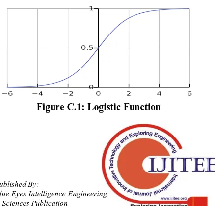
C. Logistic Regression: Logistic regression is one of the

techniques that is used to conduct a regression analysis on certain input parameters which are binary. The logistic regression function depicted in Fig C.1 is mainly focused on the sigmoidal function, which is at the core of the entire method. It maps out the characteristics of any given input data in a S-shaped format between the values of 0 and 1. It was originally developed by statisticians in order to study human population growth within in a controlled environment. It has been enhanced since then to suit other domains and accurately map their parameters.

International Journal of Innovative Technology and Exploring Engineering (IJITEE) ISSN: 2278-3075, Volume-8 Issue-7, May, 2019

Eq. (C.1)

Equation (C.1) is the mathematical definition of logistic

function for a given point X=( )

In n-dimensional space. This equation can also be written as Eq(C.2).

Eq. (C.2)

D. Decision Tree Classifier: Decision trees can be used

for problems in both regression and classification. The classification tree and the regression tree are very similar in nature but the main difference is that classification tree is meant to predict the qualitative response while the regression tree is meant for a quantitative response. Decision tree classifiers like the regular decision trees will reject other classes until the solution class is found and labeled. For this to occur, we must initially split our feature spaces into a set of unique regions with classes. While the Binary trees are the simplest form, where the tree splits off the feature space into two different parts based upon a threshold that is defined by the user. The class is assigned with a feature vector and a path is also specified to its location. Designing a classification tree, we require the use of the splitting criterion, class assignment rule, and the stop-splitting rule.

E. Support Vector Machines: The main purpose of the

SVM algorithm is to search for a hyperplane in an N-Dimensional space so that it can categorize a set of data points. In an SVM, we are given a set of data points that are needed to be classified but finding the right hyperplane for the sample is quite difficult. There are quite a lot of hyperplanes that can be chosen. However, If the wrong hyperplane is chosen, the results can be catastrophic due to the incorrect classification of the training data. Now, the hyperplane works by considering the maximal margin hyperplane, which is basically the greatest distance from the data points. By finding the hyperplane which has the greatest between the points but closest to the training data, it allows to accurately classify the input data. The SVM algorithm can be basically visualized a linear curve that classifies data points based upon where they lie upon the hyperplane. The drawback with SVM is that outlier datapoints can severely hinder the accuracy rate of the entire algorithm.

_{Eq. (E.1)}

Eq. (E.1) is the mathematical definition of hyperplane in

n-dimensional space. Let X=( ) be a

point in that n-dimensional space.

If then the point lies

above the hyperplane. If

Point lies below the plane. So by calculating equation (E.1) one can know on which side of the hyperplane the point lies, in other words we can determine which class it belongs to.

III. RESULTS

A. Artificial Neural Networks: In our experimentation

we have constructed a two-layer neural network. The architecture of our ANN model is depicted in Figure A.1. It clearly elucidates the fact that we have used a two-layer neural network and augmented dropout layer to escalate the overfitting issues.

Figure A.1 - Architecture of ANN

Overfitting: We have also implemented a neural network

without using any regularizations or drop out and omitted preprocessing steps like normalizing data and feature engineering. The resultant model proved to be very inaccurate, time consuming and inconsistent.

Figure A.2 – Before preprocessing

Figure A.2 illustrate the outcome of a neural network model which was trained on non-processed data and with no drop out layers. Though the train accuracy proved to be good and peaked 90% accurate, validation results seems not satisfying. The model has shown good results for training data than the test sample. Our model is yielding better results with the training set rather than the test set. This particular result is occurring due to overfitting of the test data.

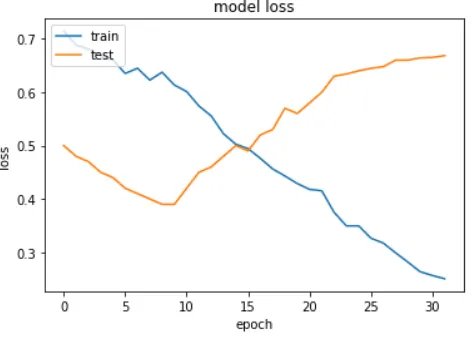
Figure A.3: Model Loss

The loss function that we considered was the binary cross entropy. When we use this function, the trained set can be viewed to be improving in the overall loss of the set but in reality, the test data suggests otherwise. The test data is actually increasing in loss when compared to trained sample. The increase in loss can be attributed to the overfitting of the data. In the above Figure A.3, as more epochs considered for the trained set, the loss decreases with the set. While, the tested set starts with a lower loss value but with the more epochs being considered, the loss of the tested set actually increases. This illustrates the drawback of the architecture and methodology that is being used. At 10 epochs, the loss both the sets are almost equal. After 10 epochs, the loss of the training set linearly decreases while the loss of the test set gradually increases. The visual representation and the statistics both confirm the overfitting of the data sets. However, this can all be fixed when we perform normalization, preprocessing, and adding dropout layers. After adding dropout layer and normalizing feature set:

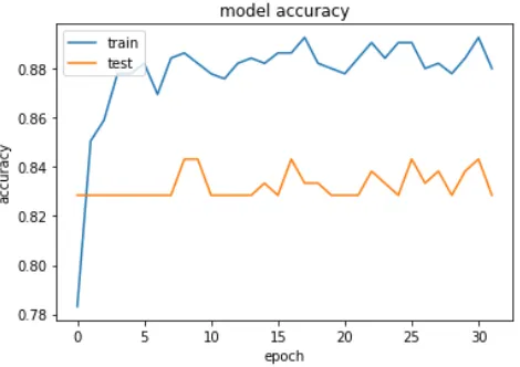
Figure A.4: Accuracy after adding Dropout

Figure A.5: Loss function results

After the addition of the preprocessing and the dropout layers, the situation for the set fares better than its previous runs. In Figure A.4, we consider a batch size and epoch size of 32. Now it can be observed that the loss of the training set decreases with more number of iterations. This was also observed in the previous model. However, in this we can also observe that the tested set also decreases in loss with the iterations. The data indicates that model accuracy of the trained set increasing exponentially with more iterations of epoch, and settling down at 81% accuracy. When we consider the accuracy for the tested set, it initially lies beneath the plane of the trained set but as the iteration increases past 5, the tested set manages to outperform the trained in accuracy. The tested set yields an accuracy that is greater than 85%. This clearly indicates that our addition of preprocessing, dropout layer and the normalizing feature set has improved the overall loss and accuracy of the model. The results of Figure A.5 also prove that our model is performing well considering the decrease of loss function with respect to epochs

B. Evaluating Logistic Regression Model:

Figure B.1: Confusion matrix

International Journal of Innovative Technology and Exploring Engineering (IJITEE) ISSN: 2278-3075, Volume-8 Issue-7, May, 2019

Eq (B.2)

Precision and recall are the two parameter that are commonly used to evaluate a classification problem. If a data point is classified as a positive by the model and is truly correct, then it considered to be a True positive(TP). If a data point is considered to be a negative but is actually positive, then it is known to be a False negative(FN). Let’s consider the use case of rainfall forecast, if the model correctly predicts a certain day to have rainfall, then it is considered to be a True positive(TP). If the model were to forecast no rainfall for a certain day but it rains on that day instead, then it is considered to be a False Negative(FN). Recall is the ability of the model to find all appropriate instances in the dataset, while the precision shows the ratio of the data points for our model that were actually pertinent. By calculating Equations B.1, B.2 and with data illustrated in Fig B.1 we get values of recall and precision respectively. The model is 96% precise and its recall value is 0.914.

Figure B.2: Performance comparison

IV. CONCLUSION

Rainfall forecast is a daunting task for any algorithm to handle. However, the algorithm that we focused on was the Artificial Neural Networks. The reason we chose ANN was because of its ability to handle larger data, such as the large batch sizes that were inputted and also allows various types of data used. This was a huge benefactor in our decision of using ANN’s. The other reason was that it performed better than other algorithms when handling inconsistences in the data such as noise or incomplete data. Inconsistences can throw off the accuracy of the algorithms by an exceptional margin. However, ANN was capable of handling these types of data. The final results in Figure B.2 agree with our choice as ANN was able to yield an accuracy of 87%. The other algorithms could reach a maximum accuracy of 86%. If we consider extremely large datasets, that 1% can make quite the difference in forecasting. Through our model, we were able to prove that ANN’s are a viable model to be used in the field of weather forecasting. They can handle large data, handle inconsistences, and yield higher accuracies. ANN is one of the true spearheads in the domain of weather forecasting.

V. FUTURE SCOPE

In future research, we intend to incorporate different ensemble techniques to combine the diversities of the models and increase the forecasting ability. We are planning to take data from different regions to increase the diversity of the data set and check which model performs well with such noisy data. The architecture of the network model will be examined further to enhance the accuracy of predictions. We intend to extend our wing in understanding of neural networks by using different neural network models like Recurrent Neural network(LSTM) and Time delay neural network(TDNN). The accuracy of the probabilistic model like Naive Bayes will be examined. In order to do so first, we need to perform discretization. Discretization algorithms like CAIM, CLIP4 converts continuous data into discrete data by grouping them into certain bins or intervals.

REFERENCES

1. Shoba G and Shobha G., “Rainfall prediction using Data Mining techniques: A Survey,” Int. J. of Engineering. and Computer. Science., vol. 3, no. 5, pp. 6206-6211, 2014

2. J.N.K. Liu, B. N. L. Li, and T. S. Dillon. ”An improved naive Bayesian classier technique coupled with a novel input solution method” [rainfall prediction]. Systems, Man, and Cybernetics, Part C: Applications and Reviews, IEEE Trans-actions, pgs:249-256, vol.31, issue-2, 2001 3. R. S. Sangari and M. Balamurugan, “A Survey on rainfall prediction

using Data Mining,” Int. J. of Computer Science and Mobile Applications., vol. 2, no. 2, pp. 84-88, 2014.

4. Kumar Abhishek, A. Kumar, R. Ranjan and S. Kumar “A rainfall prediction model using artificial neural network”, IEEE Control and System Graduate Research Colloquium (ICSGRC), pgs: 82-87, 2012 5. Juan Beltrn-Castro, Juliana Valencia-Aguirre, Mauricio Orozco-Alzate,

Germn Castellanos-Domnguez, and Carlos M. Travieso-Gonzlez, “Rainfall Forecasting Based on Ensemble Empirical Mode Decomposition and Neural Networks” Advances in Computational Intelligence, number 7902 in Lecture Notes in Computer Science, pages 471-480, 2013.

6. S. Renuga Devi, P. Arulmozhivarman, C. Venkatesh and Pranay Agarwal “Performance comparison of artificial neural network models for daily 7. rainfall prediction”, International Journal of Automation and Computing,

Volume 13, Issue 5, pp417-427,2016

8. D. R. Nayak, A. Mahapatra, and P. Mishra, “A Survey on rainfall prediction using Artificial Neural Network,” Int. J. of Computer Applications, vol. 72, no. 16, pp. 32-40, 2013.

9. N. S. Philip and K. B. Joseph, “A Neural Network tool for analyzing trends in rainfall,” Comput. & Geosci.,vol. 29, no. 2, pp. 215-223, 2003 10.G. Zhang, B. E. Patuwo, and M. Y. Hu, “Forecasting with Artificial Neural Networks:: The state of the art,” Int J. of forecasting, vol 14, no. 1, pp. 35-62, 1998

11.S. Chattopadhyay and M. Chattopadhyay, “A Soft Computing technique in rainfall forecasting,” Int. Conf. on IT, HIT, pp. 19-21, 2007 12.B. Neyshabur, R. Tomioka, and N. Srebro, “Norm-based capacity control

in neural networks.” in COLT, 2015, pp. 1376–1401