PP 2007 11: A Fully Connectionist Model Generator for Covered

A Fully Connectionist Model Generator for Covered First-Order Logic Programs

Sebastian Bader

and

Pascal Hitzler

and

Steffen H¨olldobler

and

Andreas Witzel

∗

_{International Center for Computational Logic, Technische Universit¨at Dresden, Germany}

_{AIFB, Universit¨at Karlsruhe, Germany}

‡

_{Institute for Logic, Language and Computation, Universiteit van Amsterdam}

Abstract

We present a fully connectionist system for the learning of first-order logic programs and the gen-eration of corresponding models: Given a program and a set of training examples, we embed the asso-ciated semantic operator into a feed-forward net-work and train the netnet-work using the examples. This results in the learning of first-order knowledge while damaged or noisy data is handled gracefully.

1

Motivation

Three long-standing open research problems in connection-ism are the questions of how to instantiate the power of symbolic computation within a fully connectionist system [Smolensky, 1987], how to represent and reason about struc-tured objects and structure sensitive processes [Fodor and Pylyshyn, 1988], and how to overcome the propositional fix-ation [McCarthy, 1988], i.e. how to use connectionist sys-tems for symbolic learning and reasoning beyond proposi-tional logic. It has been shown that feed-forward networks are universal approximators and that artificial neural networks are Turing complete. Thus we know that symbolic computation is possible in principle, but at the same time the mentioned results are mainly theoretical.

Here we are concerned with the model generation for first-order logic programs, i.e. sets of rules which may contain variables ranging over infinite domains. Our approach is based on the following ideas first expressed in [H¨olldobleret al., 1999]: Various semantics of logic programs coincide with fixed points of associated semantic operators. Given that the semantic operator is continuous on the reals, the operator can be approximated arbitrarily well by a feed-forward network. In addition, if the operator is a contraction, then its fixed point can be computed by a recurrent extension of the feed-forward network.

Until now this approach was also purely theoretical for the first-order case. In this paper we show how feed-forward net-works approximating the semantic operator of a given first-order logic program can be constructed, we show how these networks can be trained using input-output examples, and we demonstrate that the obtained connectionist system is robust against damage and noise. In particular, and after stating

necessary preliminaries in Section 2, we make the follow-ing novel contributions in Section 3: We define a new multi-dimensional embedding of semantic operators into the reals, we construct a feed-forward network to approximate these operators and we present a new learning method using do-main knowledge. The resulting system is evaluated in Sec-tion 4. Finally, we draw some conclusions and point out what needs to be done in the future in Section 5. For an overview of related work we refer to [d’Avila Garcezet al., 2002] and [Bader and Hitzler, 2005].

2

Preliminaries

In this section, some preliminary notions from logic program-ming and connectionist systems are presented, along with the Core Method as one approach to integrate both paradigms.

2.1

First-Order Logic Programs

Alogic programover some first-order languageLis a set of clausesof the formA ←L1∧ · · · ∧Ln,Ais anatominL,

and theLi areliteralsinL, that is, atoms or negated atoms.

Ais called theheadof the clause, theLiare calledbody lit-erals, and their conjunctionL1∧ · · · ∧Lnis called thebody

of the clause. Ifn= 0,Ais called afact. A clause isground if it does not contain any variables.Local variablesare those variables occurring in some body but not in the correspond-ing head. A logic program iscoveredif none of the clauses contain local variables.

Example 1. The following is a covered logic program which will serve as our running example.

e(0). % 0 is even

e(s(X))←o(X). % the successor s(X) of an odd X is even o(X)← ¬e(X). %Xis odd if it is not even

TheHerbrand universeULis the set of all ground terms of

L, theHerbrand baseB_Lis the set of all ground atoms, which we assume to be infinite – indeed the case of a finiteB_Lcan be reduced to a propositional setting. Aground instanceof a literal or a clause is obtained by replacing all variables by terms fromU_L. For a logic programP,G(P)denotes the set of all ground instances of clauses fromP.

Alevel mappingis a function assigning a natural number

if there exists a level mapping | · |such that for all clauses A←L1∧· · ·∧Ln∈ G(P)we have|A|>|Li|for1≤i≤n.

Example 2. Consider the program from Example 1 and letsn denote then-fold application ofs. With|e(sn(0))|:= 2n+ 1

and|o(sn(0))|:= 2n+ 2, we find thatPis acyclic.

A(Herbrand) interpretationI is a subset ofBL. Those atomsAwithA ∈ Iare said to betrueunderI, those with A∈ Iare said to befalseunderI. I_Ldenotes the set of all interpretations. An interpretationIis a(Herbrand) modelof a logic programP (in symbols: I |= P) ifIis a model for each clause inG(P)in the usual sense.

Example 3. For the program P from Example 1 we have M :={e(sn(0))|neven} ∪ {o(sm(0))|modd} |=P.

Given a logic programP, the single-step operator TP : IL → ILmaps an interpretationIto the set of exactly those atomsA for which there is a clause A ← body ∈ G(P)

such that the body is true underI. The operatorTP captures

the semantics ofP as the Herbrand models of the latter are exactly the pre-fixed points of the former, i.e. those interpre-tationsIwithTP(I)⊆I. For logic programming purposes it is usually preferable to consider fixed points ofTP, instead of

pre-fixed points, as the intended meaning of programs. These fixed points are calledsupported modelsof the program [Apt et al., 1988]. In Example 1, the (obviously intended) model M is supported, whileBLis a model but not supported.

Logic programming is an established and mature paradigm for knowledge representation and reasoning (see e.g. [Lloyd, 1988]) with recent applications in areas like rational agents or semantic web technologies (e.g. [Angele and Lausen, 2004]).

2.2

Connectionist Systems

Aconnectionist systemis a network of simple computational units, which accumulate real numbers from their inputs and send a real number to their output. Each unit’s output is con-nectedto other units’ inputs with a certain real-valuedweight. Those units without incoming connections are called input units, those without outgoing ones are calledoutput units.

We will consider 3-layered feed-forward networks, i.e. net-works without cycles where the outputs of units in one layer are only connected to the inputs of units in the next layer. The first and last layers contain the input and output units respec-tively, the intermediate layer is called thehidden layer.

Each unit has aninput functionwhich uses the connections’ weights to merge its inputs into one single value, and an out-put function. An example for a so-calledradial basisinput function is(w, x ) → n_i=1(xi−wi)2, where the xi are the inputs and thewiare the corresponding weights. Possible

output functions are the sigmoidal function (x→ ₁₊1_e−x, for the hidden layer) and the identity (x→x, usually used in the output layer). If only one unit of a layer is allowed to output a value= 0, the layer implements awinner-take-allbehavior. Connectionist systems are successfully used for the learn-ing of complex functions from raw data called trainlearn-ing sam-ples. Desirable properties include robustness with respect to damage and noise; see e.g. [Rojas, 1996] for details.

2.3

The Core Method

In [H¨olldobler and Kalinke, 1994; Hitzler et al., 2004] a method was proposed to translate a propositional logic pro-gramPinto a neural network, such that the network will set-tle down in a stable state corresponding to a model of the pro-gram. To achieve this goal, the single-step operatorTP

asso-ciated withPwas implemented using a connectionist system. This general approach is nowadays called theCore Method [Bader and Hitzler, 2005].

In [H¨olldobleret al., 1999], the idea was extended to first-order logic programs: It was shown that theTP-operator of acyclic programs can be represented as a continuous function on the real numbers. Exploiting the universal approximation capabilities of 3-layered feed-forward networks, it was shown that those networks can approximateTP up to any given

ac-curacy. However, no algorithms for the generation of the net-works from given programs were presented. This was finally done in [Baderet al., 2005] in a preliminary fashion.

3

The FineBlend System

In this section we will first discuss a new embedding of in-terpretations into vectors of real numbers. This extends the approach presented in [H¨olldobleret al., 1999] by computing m-dimensional vectors instead of a single real number, thus allowing for a higher and scalable precision. Afterwards, we will show how to construct a connectionist system approxi-mating theTP-operator of a given programP up to a given

accuracyε. As mentioned above, in [Baderet al., 2005] first algorithms were presented. However, the accuracy obtainable in practice was limited through the use of a single real num-ber for the embedding. The approach presented here allows for arbitrarily precise approximations. Additionally, we will present a novel training method, tailored for our specific set-ting. The system presented here is a fine blend of techniques from theSupervised Growing Neural Gas (SGNG)[Fritzke, 1998] and the approach presented in [Baderet al., 2005].

3.1

Embedding

Obviously, we need to link the space of interpretations and the space of real vectors in order to feed the former into a connectionist system. To this end, we will first extend level mappings to a multi-dimensional setting, and then use them to represent interpretations as real vectors.

Definition 4. Anm-dimensional level mappingis a bijective function · : BL → (N+,{1, . . . , m}). For A ∈ BL, if A= (l, d), thenlanddare calledlevelanddimensionof A, respectively. Again, we define¬A:=A.

Definition 5. Letb ≥ 3 and letA ∈ BL be an atom with A = (l, d). The m-dimensional embedding ι : BL →

Rm_{and its extensionι : I}

L →Rmare defined asι(A) :=

(ι1(A), . . . , ιm(A))where

ιj(A) :=

b−l ifj=d

0 otherwise and ι(I) :=

A∈I

ι(A).

With Cmwe denote the set of all embedded interpretations, i.e.Cm:={ι(I)|I∈ IL} ⊂Rm.1

1

x

0.¯3

x

0.¯3

y

0.¯3

ι(M)

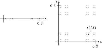
Figure 1:C1(left) andC2(right) forb= 4andMfrom Ex. 6.

x y

;

x y

;

x y

;

x y

Figure 2: The first steps while constructing the limitC2.

Example 6. Using the 1-dimensional level mapping from Example 2, we obtain C1 as depicted in Figure 1 on the left. Using the 2-dimensional level mappinge(sn(0)) := (n+ 1,1) ando(sn(0)) := (n+ 1,2), we obtainC2 as depicted on the right and ι(M) = (0.1010b,0.0101b) ≈

(0.2666667,0.0666667)for the embedding ofM.

For readers familiar with fractal geometry, we note thatC1 is the classical Cantor set andC2the 2-dimensional variant of it [Barnsley, 1993]. Obviously,ιis injective for a bijec-tive level mapping and it is bijecbijec-tive onCm. Using them -dimensional embedding, theTP-operator can be embedded

into the real vectors to obtain a real-valued functionfP.

Definition 7. Them-dimensional embedding ofTP, namely fP :Cm→Cm, is defined asfP(x) :=ιTPι−1(x).

Them-dimensional embedding ofTP is preferable to the

one introduced in [H¨olldobleret al., 1999] and used in [Bader et al., 2005], because it allows for scalable approximation precision on real computers. Otherwise, only 16 atoms could be represented with 32 bits.

Now we introducehyper-squareswhich will play an im-portant role in the sequel. Without going into detail, Figure 2 shows the first 4 steps in the construction ofC2. The big square is first replaced by2m shrunken copies of itself, the result is again replaced by2msmaller copies and so on. The limit of this iterative replacement isC2. We will useCm_i to denote the result of the i-th replacement, i.e. Figure 2 de-pictsC2₀,C2₁,C2₂andC2₃. Again, for readers with background in fractal geometry we note, that these are the first 4 appli-cations of an iterated function system [Barnsley, 1993]. The squares occurring in the intermediate results of the construc-tions are referred to ashyper-squaresin the sequel. Hl

de-notes a hyper-square of levell, i.e. one of the squares occur-ring inCm_l . An approximation ofTP up to some levellwill

yield a function constant on all hyper-squares of levell.

Definition 8. Thelargest exclusive hyper-squareof a vector u ∈Cm0 and a set of vectorsV = {v1, . . . , vk} ⊆ Cm0 , de-noted by Hex(u, V), either does not exist or is the hyper-squareHof least level for whichu∈HandV∩H =∅. The smallest inclusive hyper-squareof a non-empty set of vectors U ={u1, . . . , uk} ⊆Cm0, denoted byHin(U), is the

hyper-squareHof greatest level for whichU ⊆H.

x

0.¯3

fP(x)

0.25 0.¯3

x

0.¯3

fQ(x)

0.25 0.¯3

Figure 3:fPfor the program from Example 1 and the

embed-ding from Example 2 is shown on the left. A piecewise con-stant approximationfQ(levell= 2) is shown on the right.

3.2

Construction

In this section, we will show how to construct a connection-ist networkN for a given covered program P and a given accuracyε, such that the dimension-wise maximum distance d(fP, fN) := maxx,j(|πj(fP(x))−πj(fN(x))|)between

the embeddedTP-operatorfPand the functionfN computed

byN is at mostε. We will use a 3-layered network with a winner-take-all hidden layer.

Withl=

−ln((b−1)ε)

ln(b) , we obtain a levellsuch that when-ever two interpretationsIandJagree on all atoms up to level lin dimensionj, we find that|ιj(I)−ιj(J)| ≤ε. For a

cov-ered programP, we can construct a finite subsetQ⊆ G(P)

such that for allI∈ IL,TP(I)andTQ(I)agree on all atoms

up to level l in all dimensions, henced(fP, fQ) ≤ ε. Fur-thermore, we find that the embeddingfQ is constant on all

hyper-squares of levell[Baderet al., 2005], i.e. we obtain a piecewise constant functionfQsuch thatd(fP, fQ)≤ε.

We can now construct the feed-forward network as follows: For each hyper-squareH of levell, we add a unit to the hid-den layer, such that the input weights encode the position of the center ofH. The unit shall output1 if it is selected as winner, and0otherwise. The weight associated with the out-put connections of this unit is the value offQ on that

hyper-square. Thus, we obtain a connectionist network approximat-ing the semantic operatorTP up to the given accuracyε. To

determine the winner for a given input, we designed a locally receptive activation function such that its outcome is smallest for the closest “responsible” unit. Responsible units here are defined as follows: Given some hyper-squareH, units which are positioned inHbut not in any of its sub-hyper-squares are calleddefault unitsofH, and they are responsible for inputs fromHexcept for inputs from sub-hyper-squares containing other units. IfHdoes not have any default units, the units po-sitioned in its sub-hyper-squares are responsible for all inputs from H as well. When all units’ activations have been (lo-cally) computed, the unit with the smallest value is selected as the winner.

The following example is taken from [Witzel, 2006] and used to convey the underlying intuitions. All constructions work form-dimensional embeddings in general, but for clar-ity the graphs here result from a1-dimensional level mapping.

Example 9. Using the program from Example 1 and the1 -dimensional level mapping from Example 2 we obtainfP and

fQfor levell= 2as depicted in Figure 3. The corresponding

3.3

Training

In this section, we will describe the adaptation of the sys-tem during training, i.e. how the weights and the structure of a network are changed, given training samples with input and desired output, in such a way that the distribution under-lying the training data is better represented by the network. This process can be used to refine a network resulting from an incorrect program, or to train a network from scratch. The training samples in our case come from the original (non ap-proximated) program, but might also be observed in the real world or given by experts. First we discuss the adaptation of the weights and then the adaptation of the structure by adding and removing units. Some of the methods used here are adap-tations of ideas described in [Fritzke, 1998]. For a more de-tailed discussion of the training algorithms and modifications we refer to [Witzel, 2006].

Adapting the weights Letxbe the input,ybe the desired output and ube the winner-unit from the hidden layer. To adapt the system, we change the output weights forutowards the desired output, i.e.wout ←η·y+ (1−η)·wout.

Fur-thermore, we moveutowards the centerc of Hin({x, u}), i.e.win ←μ·c+ (1−μ)·win, whereη andμare

prede-fined learning rates. Note that the winner unit is not moved towards the input but towards the center of the smallest hyper-square including the unit and the input. The intention is that units should be positioned in the center of the hyper-square for which they are responsible.

Adding new units The adjustment described above enables a certain kind of expansion of the network by allowing units to move to positions where they are responsible for larger ar-eas of the input space. A refinement now should take care of densifying the network in areas where a great error is caused. Therefore, when a unituis selected for refinement,2we try to figure out the area it is responsible for and a suitable position to add a new unit.

Ifuoccupies a hyper-square on its own, then the largest such hyper-square is considered to beu’s responsibility area. Otherwise, we take the smallest hyper-square containingu. Nowuis moved to the center of this area, and some informa-tion gathered byuis used to determine a sub-hyper-square into whose center a new unit is placed, and to set up the out-put weights for the new unit.

Removing inutile units Each unit maintains a utility value, initially set to1, which decreases over time and increases only if the unit contributes to the network’s output.3 If a unit’s utility drops below a threshold, the unit will be removed.

3.4

Robustness

The described system is able to handle noisy data and to cope with damage. Indeed, the effects of damage to the system are

2_{The error for a given sample is ascribed to the winner unit. After}

a predefined number of training cycles, the unit with the greatest accumulated error is refined, if the error exceeds a given threshold.

3

The contribution of a unit is the expected increase of error if the unit would be removed [Fritzke, 1998].

0.01 0.1 1 10 100

0 2000 4000 6000 8000 10000 0 10 20 30 40 50 60 70 80

error #units

#examples

#units (FineBlend 1) error (FineBlend 1) #units (FineBlend 2) error (FineBlend 2)

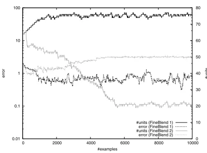
Figure 4: FineBlend 1 versus FineBlend 2.

quite obvious: If a hidden unitufails, the receptive area is taken over by other units, thus only the specific results learned foru’s receptive area are lost. While a corruption of the input weights may cause no changes at all in the network function, generally it can alter the unit’s receptive area. If the output weights are corrupted, only certain inputs are effected. If the damage to the system occurs during training, it will be re-paired very quickly as indicated by the experiment reported in Section 4.3. Noise is generally handled gracefully, because wrong or unnecessary adjustments or refinements can be un-done in the further training process.

4

Evaluation

In this section we will discuss some preliminary experiments. In the diagrams, we use a logarithmic scale for the error axis, and the error values are relative toε, i.e. a value of1 desig-nates an absolute error ofε. For incorrect network initializa-tion, we used the following wrong program:

e(s(X))← ¬o(X). o(X)←e(X).

Training samples were created randomly using the semantic operator of the program from Example 1.

4.1

Variants of Fine Blend

0.01 0.1 1 10 100

0 2000 4000 6000 8000 10000 12000 14000 0 20 40 60 80 100 120 140

error #units

#examples

#units (FineBlend 1) error (FineBlend 1) #units (SGNG) error (SGNG)

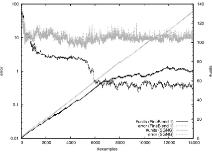
Figure 5: FineBlend 1 versus SGNG.

4.2

Fine Blend versus SGNG

Figure 5 compares FineBlend 1 with SGNG [Fritzke, 1998]. Both start off similarly, but soon SGNG fails to improve fur-ther. The increasing number of units is partly due to the fact that no error threshold is used to inhibit refinement, but this should not be the cause for the constantly high error level. The choice of SGNG parameters is rather subjective, and even though some testing was done to find them, they might be far from optimal. Finding the optimal parameters for SGNG is beyond the scope of this paper; however, it should be clear that it is not perfectly suited for our specific application. This comparison to an established generic architecture shows that our specialized architecture actually works, i.e. it is able to learn, and that it achieves the goal of specialization, i.e. it outperforms the generic architecture in our specific setting.

4.3

Unit Failure

Figure 6 shows the effects of unit failure. A FineBlend 1 network is (correctly) initialized and refined through train-ing with 5000 samples, then one third of its hidden units are removed randomly, and then training is continued as if noth-ing had happened. The network proves to handle the damage gracefully and to recover quickly. The relative error exceeds

1only slightly and drops back very soon; the number of units continues to increase to the previous level, recreating the re-dundancy necessary for robustness.

4.4

Iterating Random Inputs

One of the original aims of the Core Method is to obtain con-nectionist systems for logic programs which, when iteratively feeding their output back as input, settle to a stable state cor-responding to an approximation of a fixed point of the pro-gram’s single-step operator. In our running example, a unique fixed point is known to exist. To check whether our system reflects this, we proceed as follows:

1. Train a network from scratch until the relative error caused by the network is below1, i.e. network outputs are in theε-neighborhood of the desired output. 2. Transform the obtained network into a recurrent one by

connecting the outputs to the corresponding inputs.

0.01 0.1 1 10 100

0 2000 4000 6000 8000 10000 12000 14000 16000 0 10 20 30 40 50 60 70 80

error #units

#examples

#units (FineBlend 1) error (FineBlend 1)

Figure 6: The effects of unit failure.

M

x

0.¯3

y

0.¯3

Figure 7: Iterating random inputs. The two dimensions of the input vectors are plotted against each other. Theε -neighborhood of the fixed pointM is shown as a small box.

3. Choose a random input vector∈Cm₀ (which is not nec-essarily a valid embedded interpretation) and use it as initial input to the network.

4. Iterate the network until it reaches a stable state, i.e. until the outputs stay inside anε-neighborhood.

For our example program, the unique fixed point ofTP is M as given in Example 3. Figure 7 shows the input space and the ε-neighborhood of M, along with all intermediate results of the iteration for 5 random initial inputs. The ex-ample computations converge, because the underlying pro-gram is acyclic [Witzel, 2006; H¨olldobler et al., 1999]. Af-ter at most6steps, the network is stable in all cases, in fact it is completely stable in the sense that all outputs stay ex-actly the same and not only within anε-neighborhood. This corresponds roughly to the number of applications of our program’sTP operator required to fix the significant atoms,

which confirms that the training method really implements our intention of learningTP. The fact that even a network

ob-tained through training from scratch converges in this sense further underlines the efficacy of our training method.

5

Conclusions and Further Work

can be learned from given training examples using a mod-ified neural gas method which exploits domain knowledge. The resulting system degrades gracefully under damage and noise, and recovers using training.

Whereas we define the embedding ι externally, in [Gust and K¨uhnberger, 2005] such embeddings are learned using ideas from category theory. In [Seda and Lane, 2005], con-nectionist systems for a covered programP are constructed by generating finite subsets ofG(P)and employing the con-structions presented in [H¨olldobler and Kalinke, 1994].

Besides a thorough comparison of these approaches much remains to be done. The presented methods and procedures involve parameters, which are set manually; we would like to find (preferably optimal) parameters automatically. We would like to extract first-order logic programs after train-ing, but all the extraction methods that we are aware of are propositional. This is a prerequisite not only to compare our method of learning semantic operators of logic programs with that of inductive logic programming, but also to complete the neural-symbolic learning cycle [Bader and Hitzler, 2005]. The investigation of realistic applications, e.g. to the learning of ontologies and other types of knowledge bases [Hitzleret al., 2005] will follow.

Acknowledgments

We would like to thank three anonymous referees for their valuable comments on the preliminary version of this pa-per. Sebastian Bader is supported by the GK334 of the Ger-man Research Foundation (DFG). Pascal Hitzler is supported by the German Federal Ministry of Education and Research (BMBF) under the SmartWeb project (grant 01 IMD01 B), and by the X-Media project (www.x-media-project.org) spon-sored by the European Commission as part of the Information Society Technologies (IST) programme under EC grant num-ber IST-FP6-026978. Andreas Witzel is supported by a Marie Curie Early Stage Research fellowship in the project GloRi-Class (MEST-CT-2005-020841).

References

[Angele and Lausen, 2004] J. Angele and G. Lausen. On-tologies in F-Logic. In S. Staab and R. Studer, editors, Handbook on Ontologies, pages 29–50. Springer, 2004. [Aptet al., 1988] K. R. Apt, H. A. Blair, and A. Walker.

To-wards a theory of declarative knowledge. In J. Minker, ed-itor,Foundations of Deductive Databases and Logic Pro-gramming, pages 89–148. Morgan Kaufmann, 1988. [Bader and Hitzler, 2005] S. Bader and P. Hitzler.

Dimen-sions of neural-symbolic integration — a structured sur-vey. In S. Artemov et al., editor,We Will Show Them: Es-says in Honour of Dov Gabbay, volume 1, pages 167–194. King’s College Publications, JUL 2005.

[Baderet al., 2005] S. Bader, P. Hitzler, and A. Witzel. In-tegrating first-order logic programs and connectionist sys-tems — a constructive approach. In A. S. d’Avila Garcez et al., editor, Proceedings of the IJCAI-05 Workshop on Neural-Symbolic Learning and Reasoning, NeSy’05, Ed-inburgh, UK, 2005.

[Barnsley, 1993] M. Barnsley. Fractals Everywhere. Aca-demic Press, San Diego, CA, USA, 1993.

[d’Avila Garcezet al., 2002] A. S. d’Avila Garcez, K. B. Broda, and D. M. Gabbay.Neural-Symbolic Learning Sys-tems — Foundations and Applications. Perspectives in Neural Computing. Springer, Berlin, 2002.

[Fodor and Pylyshyn, 1988] J. A. Fodor and Z. W. Pylyshyn. Connectionism and cognitive architecture: A critical anal-ysis. In Pinker and Mehler, editors,Connections and Sym-bols, pages 3–71. MIT Press, 1988.

[Fritzke, 1998] B. Fritzke. Vektorbasierte Neuronale Netze. Habilitation, Technische Universit¨at Dresden, 1998. [Gust and K¨uhnberger, 2005] H. Gust and K.-U.

K¨uhnber-ger. Learning symbolic inferences with neural networks. In B. Bara, L. Barsalou, and M. Bucciarelli, editors, CogSci 2005: XXVII Annual Conference of the Cognitive Science Society, pages 875–880, 2005.

[Hitzleret al., 2004] P. Hitzler, S. H¨olldobler, and A. K. Seda. Logic programs and connectionist networks. Jour-nal of Applied Logic, 3(2):245–272, 2004.

[Hitzleret al., 2005] P. Hitzler, S. Bader, and A. d’Avila Garcez. Ontology leaning as a use case for neural-sym-bolic integration. In A. Garcez et al., editor,Proceedings of the IJCAI-05 Workshop on Neural-Symbolic Learning and Reasoning, NeSy, 2005.

[H¨olldobler and Kalinke, 1994] S. H¨olldobler and Y. Kalin-ke. Towards a massively parallel computational model for logic programming. InProceedings ECAI94 Workshop on Combining Symbolic and Connectionist Processing, pages 68–77. ECCAI, 1994.

[H¨olldobleret al., 1999] S. H¨olldobler, Y. Kalinke, and H.-P. St¨orr. Approximating the semantics of logic programs by recurrent neural networks.Applied Intelligence, 11:45–58, 1999.

[Lloyd, 1988] J. W. Lloyd. Foundations of Logic Program-ming. Springer, Berlin, 1988.

[McCarthy, 1988] J. McCarthy. Epistemological challenges for connectionism. Behavioural and Brain Sciences, 11:44, 1988.

[Rojas, 1996] Raul Rojas.Neural Networks. Springer, 1996. [Seda and Lane, 2005] Anthony K. Seda and Maire Lane. On approximation in the integration of connectionist and logic-based systems. InProceedings of the Third Interna-tional Conference on Information (Information’04), pages 297–300, Tokyo, November 2005. International Informa-tion Institute.

[Smolensky, 1987] P. Smolensky. On variable binding and the representation of symbolic structures in connectionist systems. Technical Report CU-CS-355-87, Department of Computer Science & Institute of Cognitive Science, Uni-versity of Colorado, Boulder, CO 80309-0430, 1987. [Witzel, 2006] A. Witzel. Neural-symbolic integration –