Partial synchronization of non-identical chaotic systems via adaptive control, with applications to modelling coupled nonlinear systems

adaptive control, with applications to modelling coupled nonlinear systems.

White Rose Research Online URL for this paper: http://eprints.whiterose.ac.uk/79677/

Version: Accepted Version

Article:

Wagg, D.J. (2002) Partial synchronization of non-identical chaotic systems via adaptive control, with applications to modelling coupled nonlinear systems. International Journal of Bifurcation and Chaos, 12 (3). 561 - 570.

https://doi.org/10.1142/S0218127402004589

[email protected] Reuse

Unless indicated otherwise, fulltext items are protected by copyright with all rights reserved. The copyright exception in section 29 of the Copyright, Designs and Patents Act 1988 allows the making of a single copy solely for the purpose of non-commercial research or private study within the limits of fair dealing. The publisher or other rights-holder may allow further reproduction and re-use of this version - refer to the White Rose Research Online record for this item. Where records identify the publisher as the copyright holder, users can verify any specific terms of use on the publisher’s website.

Takedown

If you consider content in White Rose Research Online to be in breach of UK law, please notify us by

PARTIAL SYNCHRONIZATION OF NON-IDENTICAL

CHAOTIC SYSTEMS VIA ADAPTIVE CONTROL,

WITH APPLICATIONS TO MODELING COUPLED

NONLINEAR SYSTEMS

David J. Wagg

Department of Mechanical Engineering, University of Bristol, Queens Building, University Walk, Bristol BS8 1TR, U.K.

May 3, 2013

Abstract

We consider the coupling of two non-identical dynamical systems using an adaptive

feed-back linearization controller to achieve partial synchronization between the two systems. In

addition we consider the case where an additional feedback signal exists between the two

systems, which leads to bidirectional coupling. We demonstrate the stability of the adaptive

controller, and use the example of coupling a Chua system with a Lorenz system, both

ex-hibiting chaotic motion, as an example of the coupling technique. A feedback linearization

controller is used to show the difference between unidirectional and bidirectional coupling.

We observe that the adaptive controller converges to the feedback linearization controller

in the steady state for the Chua-Lorenz example. Finally we comment on how this type of

partial synchronization technique can be applied to modeling systems of coupled nonlinear

subsystems. We show how such modeling can be achieved where the dynamics of one system

is known only via experimental time series measurements.

Running title:Partial synchronization of non-identical systems

1

Introduction

The problem of synchronizing two identical dynamical systems has been studied by many

authors, for example: Ashwin et al. (1994); Kozlov & Shalfeev (1996), Ashwin (1998) and Yang & Duan (1998), following the work of Pecora & Carroll (1990). When this is achieved using

adaptive control type methods, the process is referred to as adaptive synchronization (John &

Amritkar 1994; Boccaletti, Farini & Arecchi 1997; Fradkov & Markov 1997; Dedieu & Ogorzalek

1997). More recently the concept of partial synchronization between two or more similar chaotic

systems has been studied (Hasler 1998; Yanchuk, Maistrenko & Mosekilde 2001). In this paper

we consider coupling two non-identical dynamical systems via partial synchronization using an

adaptive synchronization technique.

A case of particular interest is when an additional feedback signal exists between the two

systems such that the coupling is bidirectional and the two systems interact dynamically, giving

rise to a complex dynamical behavior. This has applications to dynamic substructuring, where

systems are modeled by coupling a set of interacting substructures together (Ohayon et al. 1997; Wagg & Stoten 2001). We demonstrate this concept using both a feedback linearization controller

and an adaptive feedback linearization controller.

In addition, we demonstrate how the adaptive controller can be designed when coupling single

and multiple variables from each of the non-identical nonlinear systems. We show that this type

of adaptive controller is stable for such a coupled system. This is demonstrated using the example

of coupling a Lorenz system with a Chua system; for similar examples see Di Benardo (1996).

In this example, we observe that the steady state adaptive controller converges to the feedback

linearization controller.

Finally we discuss applications to modeling dynamical systems composed of a set of coupled

nonlinear dynamical systems. We discuss how partial synchronization can be used to achieve this

type of modeling. We also discuss how the concepts of synchronizing dynamical systems, (Ashwin

1998) can be used to monitor the performance of the controller producing the coupling and hence

2

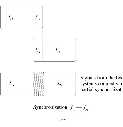
Partial synchronization for non-identical systems

We consider two non-identical dynamical systems, one with state variable x ∈ Rp_{, and the}

second, with state variable y∈ Rq_{, with governing equations of the general form}

˙

x(t) =f1(x, t),

˙

y(t) =f2(y, t).

(1)

In general, we consider that the dynamics of the two systems are nonlinear and that there is no

cross coupling between the two sets of state variables. We define a coordinate subset ofx,xs ∈ Rn,

and similarly ys ∈ Rn, which represent the coordinates which require synchronization to achieve

coupling between the two systems. So, we will consider the class of systems for which equation 1

can be expressed as

˙

xn(t) =f11(xn, xs, t)

˙

xs(t) =f12(x_n, x_s, t)

˙

ys(t) =f21(yn, ys, t)

˙

yn(t) = f22(y_n, y_s, t)

(2)

where xn = {xi ∈ x : xi ∈/ xs} and xi denotes the ith element of x, and likewise yn = {yi ∈ y :

yi ∈/ ys}. Then ifxs →ys as t→ ∞we say that the systems is partially synchronized. When such

partial synchronization occurs a coupled system is formed which is shown schematically in figure

1. The case where xs =x and ys =y is the standard synchronization problem (Pecora & Carroll

1990).

To achieve partial synchronization, we need to synchronize the dynamics of f12 and f21. Thus

we add a controller, to the coupled system, such that equation 2 can be written as

˙

xn(t) =f11(x_n, x_s, t)

˙

xs(t) =f12(xn, xs, t) +g(u, t)

˙

ys(t) =f21(y_n, y_s, t)

˙

yn(t) =f22(yn, ys, t)

(3)

whereuis the control signal, andg(·) represents the controller function. In this form, the dynamics

of f21 can be thought of as the reference model (Landau 1979), which we want f12 +g(u, t) to

replicate andf12 represents the plant.

So, in the formulation of equation 3, a part of system 1 will be forced to behave like part of

of systems 2. In this case, an additional feedback signal betweenf1 andf2 can be used to represent

the coupling. We represent it by adding a coupling function to f21, such that

˙

xn(t) =f11(xn, xs, t)

˙

xs(t) = f12(x_n, x_s, t) +g(u, t)

˙

ys(t) =f21(yn, ys, t) +c(xn, xs, t)

˙

yn(t) =f22(y_n, y_s, t)

(4)

In the case wheref1 is a physical system andf2 is an analytical model the dynamics off11can be

assumed to be unknown, and c(xn, xs, t) would typically be a recorded time series from f11. The

functions f22 and f21 must be known explicitly, so that they can be computed numerically, and

the structure of the f12 must be known. Knowledge of specific parameter values is not required,

as the adaptive controller can be applied without this information. If c= 0 the coupling between

the two systems (via partial synchronization) is effectively unidirectional, whereas if c 6= 0 the

coupling is bidirectional; examples will be discussed in section 3.1, 4.1 and 5.1. We note also that

the analysis in this section is for autonomous systems, however it is possible to apply this analysis

to some non-autonomous systems (Wagg & Stoten 2001) which we briefly discuss in section 5.1.

2.1 Controller design

To design a controller for the system we first reduce equation 4 to the form

˙

xs(t) =f12(d1(t), x_s, t) +g(u, t)

˙

ys(t) =f21(d2(t), ys, t) +c(t)

(5)

where the dynamics of xn and yn are now represented by the functions d1 and d2 respectively,

which we assume act as disturbances. Then we can formulate the error dynamics for the system

such that

˙

e(t) =f21(d2(t), ys, t)−f12(d1(t), xs, t) +c(t)−g(u, t) . (6)

where the error, e=ys−xs. This can then be expressed as

˙

e(t) = ∆f(t) +c(t)−g(u, t) . (7)

where ∆f(t) = f21−f12. For effective performance of the controller, we require that the

equi-librium, e = 0 is stable. From equation 7 we see that the controller has to compensate for the

In this formulation there are two additional disturbances, d1, d2. These functions are not

external disturbances in the ordinary sense, but signals from some other part of the coupled

system. As a result, the controller must compensate for the influence of these additional signals.

3

Single variable coupling

Let us first consider the case where only a single coordinate of f1 and f2 is to be synchronized,

and therefore e is scalar in this case. Then we can write the error dynamics as

˙

e(t) =−λe+L−g(u, t), (8)

where L = ∆f +λe+c, and λ > 0. This type of formulation is possible with a wide variety of

both linear and nonlinear systems (Di Benardo 1996), and this requirement is therefore not overly

restrictive. It is clear from equation 8 that (L−g1(u, t))→0, and λ >0 will stabilize the required

equilibrium,e = 0. ThereforeLis the feedback linearization controller for the system (Di Benardo

1996).

For the class of systems considered in this work, L can be expressed as L = k∗

ξ, where k∗

represents a set of (constant) parameters, and ξthe vector of coupling variables. For such systems

we use an adaptive controller which has essentially the same form asL, g(u, t) =u=k(t)ξ, where

k(t) is the adaptive gain. Using these definitions enables us to express equation 8 as

˙

e(t) =−λe+φ(t)ξ(t), (9)

where φ(t) =k∗

−k(t) is the parameter error. We then need to find an expression for k(t) which

stabilizes the system such that φ(t)→0 as t→ ∞. This we can achieve by choosing a Lyapunov

function of the form

V(t) = e

2

2 +

φφT

2γ , (10)

where γ is the controller gain. Then the derivative of V with respect to time is

˙

V(t) = e(−λe+φ(t)ξ(t)) + 1

γφφ˙

T_{, (11)}

such that choosing ˙φT _{=−γeξ, results in ˙V =−λe}2

which implies that the controller is globally

asymptotically stable for λ > 0. As k∗

is constant, ˙φT _{= −k}˙T _{= −γeξ, such that the adaptive}

gain becomes

kT _=γ

Z t

t=_t0

(Sastry & Bodson 1989). Thus k(t)→k∗

as φ →0 and e→ 0. Note: providing φ → 0, the final

adaptive gain values correspond to the unknown set of system parametersk∗

. In generalk(t)→k∗

providing the adaptive controller has a persistently exciting signal (see for example Sastry (1999).

From qualitative examination of our numerical simulations in this paper this is nearly always the

case.

Finally, there is an extra effect on the stability of the partially synchronized systems due to

the signals d1, d2 and c. For global asymptotic stability that these signals must remain bounded.

As they are dependent on state variables, they can only become unbounded if the system becomes

unstable. Therefore providing the system reaches a stable state with d1, d2 and c bounded the

system will remain stable.

3.1 Example coupling the Chua and Lorenz systems

We now consider an example of coupling a Chua system with a Lorenz system. In this example

(for an example of adaptive control using similar systems see Stoten & Di Bernardo (1996)), we

use a Chua system defined as

˙

x1 =α1(x2−x1) +α2x1−α3(|x1+ 1| − |x1 −1|)

˙

x2 =x1−x2+x3

˙

x3 =−δx2

(13)

and a Lorenz system

˙

y1 =−σ(y1−y2)

˙

y2 =ry1−y2−y1y3

˙

y3 =y1y2−by3

(14)

To ensure that both systems are chaotic, we select the parameter values: α1 = 10, α2 = 0.68,

α3 = 0.59,δ =−14.87,σ= 10, r= 28 andb= 8/3. Initial conditions for the system were selected

asx1(0) = 1.1,x2(0) = 1.0,x3(0) = 7.0,y1(0) =−1.1,y2(0) =−1.0 andy1(0) =−5.0. This choice

of parameters and initial conditions is arbitrary: control can be applied for any parameter values.

Now let us consider the case when we wish to couple (i.e. synchronize) x3 and y1. Thus, we

define xn= [x1, x2]T,xs =x3,ys =y1 and yn = [y2, y3]. Then

f11 =





α1(x2−x1) +α2x1 −α3(|x1+ 1| − |x1−1|)

x1−x2+x3



and

f22=





ry1−y2−y1y3

y1y2−by3



. (16)

The reference model is f21, and therefore the control signal must be applied to f12 such that

f12 =−δx2+u. (17)

Thus we are coupling the two systems by controlling f12 to follow f21. So in this case we can

think of the Lorenz system as the master or forcing system and the Chua as a slaved system, such

that the coupling is unidirectional. We can introduce bidirectional coupling by adding a coupling

function, c(t), to the Lorenz system, such that the reference f21 can be written as

f21 =−σ(y1−y2) +c(t) (18)

where cis set to zero in the unidirectional case.

3.1.1 Feedback linearization controller

To demonstrate the difference between unidirectional, and bidirectional coupling, we first use

a controller based on feedback linearization (see for example Di Benardo (1996)). To design such

a controller we need to know ∆f explicitly, which in this example is

∆f =f21−f12 =−σy1 +σy2+c+δx2−u. (19)

The error variable e=ys−xs=y1−x3, so that equation 19 can be expressed as

∆f =f21−f12=−λe+σ(y2−x3) +c+δx2−u, (20)

where λ=σ in this case. So, in this example as σ > 0, we can write

∆f =f21−f12 =−σe+L−u, (21)

which is equivalent to the right hand side of equation 9. Thus for feedback linearization we set

u=L=σ(y2−x3) +c+δx2.

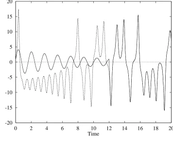
A numerical simulation of the unidirectional (master-slave) system, c = 0, is shown in figure

2. Here the response of x3 from the Chua system is shown as a solid line, while the response y1

of the Lorenz system is shown as a dashed line. The controller is initially turned off u = 0, and

controller is turned on. The two selected coordinates from the systems quickly synchronize, with

the Chua x3 coordinate slaved to the Lorenz y1 coordinate.

In figure 3 we show a simulation for the bidirectional case, when c = x3. Here the response

of x3 from the Chua system is shown as a solid line, while the response y1 of the Lorenz system

is shown as a chain dotted line. In addition we have plotted the output from the Lorenz system

(dashed line) for the c= 0 case as a comparison. Again the control is turned on at t = 12, and

the two systems quickly become synchronized. This time however the dynamics are not slaved

to the Lorenz system. The bidirectional coupling produces interaction between the two systems,

such that the dynamical behavior is not the same as the master slave example. This can be seen

in figure 3 from the deviation of the synchronized system from the Lorenz system aftert = 12.

3.1.2 Adaptive feedback linearization control

Now we consider the same synchronization problem using an adaptive controller. To achieve this

we have to express L, the feedback linearization controller, as a product of a unknown parameter

vector, k∗

and a coupling variable vector, ξ. Thus

L=σ(y2−x3) +δx2+c={σ, δ, β}

        

y2−x3

x2 c          (22)

so that the coupling variable vector is ξ = {(y2 −x3), x2, c}T and the parameter vector is k ∗

=

{σ, δ, β = 1}, and β is a dummy parameter variable.

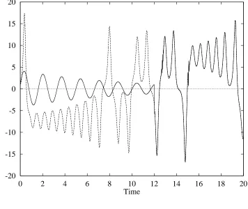
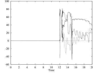
The response of the system is shown in figure 4, where again the controller was initiated at

time t = 12. The evolution of the adaptive gains k = {k1, k2, k3}T which were all initiated at

zero, is shown in figure 5 where a controller gain of γ = 100 in equation 12 was found sufficient to

achieve fast adaption. We can see from figure 5 that during the first 8 seconds of adaption gains

vary significantly. However, at time t= 1000, the adaptive gains are approximately constant with

values close to k = {k1 ≈ 10, k2 ≈ 15, k3 ≈ 1}T. Thus we see that k1 → σ, k2 → δ and k3 →β.

Thus via the relation u=k(t)ξ(t) we see that the steady state adaptive controller is the same as

4

Multi-variable coupling

For multi-variable coupling between nonlinear systems controller design is more difficult. Here,

we take the approach of analyzing the stability of the system in a partially decentralized form.

This means that the linear error coordinates are decoupled, but nonlinear coupling exists.

Thus for a system of N error equations, the ith equation can be written in a similar form to

equation 9 as

˙

ei(t) = −λiei+φi(t)ξ(t), (23)

where φi(t) is an (1×m) parameter error vector, and ξ is the (m×1) coordinate coupling vector

for all N error states. We choose a Lyapunov function of the form

V(t) =

N X i=1 (e 2 i 2 +

φiφTi

2γi

), (24)

where γi is the controller gain. Then the derivative of V with respect to time is

˙

V(t) =

N

X

1

(ei(−λiei +φi(t)ξ(t)) +

1

γi

φiφ˙Ti ), (25)

such that choosing ˙φT

i = −γieiξ, results in ˙V = PN1 −λie 2

i which implies that the controller is

globally asymptotically stable. Therefore ˙φT

i =−k˙T =−γieiξ.

4.1 Example of multi-variable coupling

We now discuss an example of coupling more than a single variable again using the Chua

and Lorenz systems as an example. In this example, two variables from each system are coupled

simultaneously.

To demonstrate this, we select x2 and y1 as the first pair of variables, and x3 and y2 as the

second pair of variables for coupling. This means that we now have two error variables,e1 =y1−x2

and e2 = y2 −x3. Unidirectional coupling only is considered, such that c = 0. In this case the

coupling functions are

f12=





x1−x2+x3

−δx2



 (26)

and

f21=





−σ(y1−y2)

ry1−y2−y1y3



Therefore

∆f =f21−f12 =





−σ(y1 −y2)−x1+x2 −x3−u1

ry1−y2−y1y3+δx2−u2



, (28)

which can be expressed as

∆f =f21−f12=





−σe1+σy2+ (1−σ)x2−x3−x1−u1

−e2 +ry1+δx2−x3−y1y3−u2



, (29)

such that we can write

˙

e1(t) =−σe1+L1−u1,

˙

e2(t) =−e2+L2−u2

(30)

Where the feedback linearization controllers are

L1 =σy2+ (1−σ)x2−x3−x1

L2 =ry1+δx2−x3−y1y3

(31)

For adaptive feedback linearization we write each Li =k

∗

iξ such that in this case

k∗

1 = [0, σ,(1−σ),−1,−1,0]

k∗

2 = [r,0, δ,−1,0,−1]

(32)

and ξ = [y1, y2, x2, x3, x1, y1y2]T. Then finally we can express equation 30 in the required format

of equation 23 by substituting ui =ki(t)ξ, giving

˙

e1(t) =−σe1 +φ1(t)ξ(t),

˙

e2(t) =−e2+φ2(t)ξ(t)

(33)

Then for this system stabilizing controllers can be applied using the gain vectors given by kT i =

γi

Rt

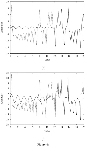
t=_t0eiξdt. The results of simulating this example are shown in figure 6. As with the previous

examples, the control is started at time t = 12. From figure 6 (a) we see that x2 become

syn-chronized with y1 very quickly after the control starts. However, the x3, y2 synchronization takes

significantly longer; approximately 2 seconds. We also find that after 1000 seconds k1 ≈ k ∗ 1, but

that k2 has not completely converged to k ∗

2. This behavior occurs because of our choice of the

λi values in this example; equation 30. For the x2, y1 synchronization λ1 = σ = 10, but for the

x3, y2 synchronization λ1 = 1. Considering the convergence when L1 −u1 = 0 and L2 −u2 = 0,

e1 = exp(−10t) while e2 = exp(−t). Therefore the error convergence of e1 will be greater than

5

Applications to modeling coupled dynamical systems

Many real life dynamical systems are composed of two or more coupled systems giving rise

to highly complex dynamics. Partial synchronization techniques can be applied to modeling such

systems in two main ways:

1. To model systems composed of a set of coupled nonlinear subsystems, where the structure

of the individual component systems is known, but the nature of the coupling is unknown.

2. To model systems composed of a set of coupled nonlinear subsystems, where information

from one (or more) of the subsystems is known only in the form of a recorded time series.

The first approach can be used to synchronize two variables from the subsystems to effect

coupling, without having to have explicit knowledge of the form of the coupling itself. The second

method has potential uses for systems where time series data is taken from an experimental source.

For example in techniques which have a numerical and experimental component to the modeling

(Oomens et al. 1993; Doneaet al. 1996; Wagg & Stoten 2001) These two modeling methods can be approached using the coupling techniques described in section 2.

5.1 Example: modeling a system of two coupled nonlinear dynamical systems

Consider the problem of modeling the dynamics of a complex dynamical system governed by

the state equation

˙

z(t) =f(z, t), (34)

where we have only partial knowledge of the form of f(z, t). We will consider the problem where

f(z, t) is composed of two parts, one for which the dynamics is known explicitly,f2, and the other,

f1 where the dynamics can be divided into; a part where the structure is known, f12, and a part

where the dynamics are known only via time series measurementsf11. This is the situation in some

numerical-experimental applications, where a physical system is acted upon by some experimental

apparatus and this is coupled with a numerical model (Wagg & Stoten 2001). So in this case the

coordinates of the apparatus would correspond to xs, and the dynamics of xn would be known

only implicitly from experimental measurements of the physical system.

To create a model off(z, t) the coordinatesxs andys need to be synchronized such thate→0.

2) as

˙

z(t) =

         ˙

xn(t)

˙

xs(t)

˙

yn(t)

         =         

f11(x_n, x_s, t)

f12(xn, xs, t)

f22(y_n, y_s, t)

        

=f(z, t). (35)

As before, this is achieved by using an adaptive control algorithm to ensure that f12 tracks f21

i.e. f12→ f21. Thus the coupled systems form a single combined model of the overall system. In

this process we will effectively reconstruct the dynamics of the experimental system (Broomhead

& King 1986; Maybhate & Amritkar 1999), while simulating the dynamics known explicitly, and

thus reconstruct the overall dynamics of the system f(z, t).

Let us consider the case where the dynamics ofxn, represented byf11are unknown in a explicit

form but are known implicitly from a set of experimental measurements in the form of time series

v(t) and w(t) such that xn = h1(v(t)) and ˙x_n = h2(w(t)). Here h_j(·) are correlation functions

which provide a relationship between the experimental measurements and state variables. In this

case equation 3, can be written as

˙

xn(t) =h2(w(t))

˙

xs(t) =f12(h1(v(t)), x_s, t) +g(u, t)

˙

ys(t) =f21(y_n, y_s, t)

˙

yn(t) =f22(y_n, y_s, t)

(36)

This set of equations can be used to form a coupled model for the overall system, by substituting

h1 =d1 andy_n=d2, we obtain equation 5, and forv(t),w(t) bounded, the stability proof follows.

In addition, whenf12andf21are synchronized, equation 36 can be reduced to the form of equation

35 to provide a combined system model.

5.1.1 Numerical-experimental example

Wagg & Stoten (2001) consider a numerical-experimental example wheref11and f12 are

physi-cal systems butf12is (approximately) linear. A force signal, F(t), betweenf11 and f12 is recorded

experimentally which represents the coupling between the two functions. For this system equation

36 can be written in the form

˙

xn(t) =f11

˙

xs(t) =Axs+Bu

˙

ys(t) =Amys+Bmyn+CmF(t)

where A, B, Am, Bm, Cm, Az, Bz and Cz are constant matrices and f11 is an unknown nonlinear

function. In this example only part of the system is nonlinear, but the development of the combined

model for the system uses a similar approach to that described here for nonlinear systems. We

note also that this system has bidirectional coupling from the application of F(t) and is

non-autonomous via the forcing signal r(t). Further details of this can be found in Wagg & Stoten

(2001).

5.2 How effective is this modeling process?

In order to measure the degree of synchronization between the coordinates xs and ys, we

monitor the error vector e =ys−xs. For effective modeling we require that the synchronization

occurs within a certain time limitation e → ǫ as t → ts, where ǫ is small. The effectiveness

of the synchronization process can be viewed geometrically by considering the phase space for

the coupled system E = {(x, y) ∈ Rp×_q

}. Then Σ = {(x, y) ∈ Rp×_q

: e = 0} represents the

synchronized subspace (Ashwin 1998) for the coupled system. The dynamics which are restricted

to the manifold Σ correspond to that of the coupled system, equation 34. Furthermore, out of

subspace dynamics correspond to failure in the synchronization (control) process. Thus we can

use the synchronization subspace to monitor the performance of the controller, and hence the

effectiveness or accuracy of the modeling process.

If we define the phase space of the overall system we are trying to model as G = {z ∈ Rk_},

then the combined model is a close approximation of the overall system if dim Σ ≈ dimG. In

other words the combined system, f1 and f2, has higher dimensional dynamics than the modeled

system, f(z, t), but by synchronizing the required set of coordinates we reduce the dynamics to

the subspace Σ which is an approximation of the overall dynamics in G. Thus we can qualitatively

identify the dynamics of the overall system by examining the dynamics in the hypersurface Σ.

5.2.1 Chua-Lorenz example

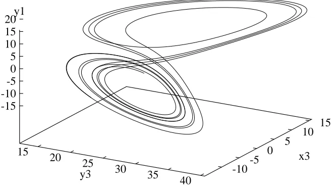
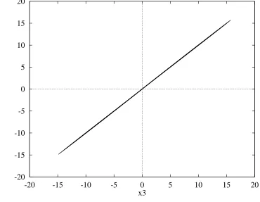
This can be demonstrated using the example from section 3.1. LetE ={(x3, y1, y3)∈R 3

}be a

subset of the complete phase space, which we can use as a visualization aid. The evolution of the

feedback coupled system in this space is shown in figure 7. In this example feedback linearization

control was used from time t = 0, and the figure shows trajectories computed from t = 40 to

t= 50. Lorenz-like dynamics can be observed, however these dynamics are in fact restricted to the

we observe no out of subspace dynamics, indicating a high level of accuracy in the coupling and

hence modeling process, which can be expected from feedback linearization control. Similar results

can be obtained using adaptive feedback linearization, however in this case some out of subspace

dynamics will occur during the transient adaption phase when t > ts.

6

Conclusions

We have considered how non-identical nonlinear dynamical systems can be coupled using partial

synchronization with the inclusion of additional feedback coupling. For applications where two

different dynamical system require coupling, a partial synchronization method can be used where

one part of the system is included using only a recorded time series. We have demonstrated how

both unidirectional and bidirectional coupling can be simulated in such a modeling process using a

feedback linearization controller. We have also demonstrated using the example of a Chua system

coupled with a Lorenz system, how an adaptive feedback linearization controller can be used to

effect such coupling. The use of an adaptive controller is significant, in that it can be used to couple

systems without explicit knowledge of the plant parameters, although a knowledge of the structure

of the plant is required. In the steady state, we observed that the adaptive controller converged

to the exact formulation of the feedback linearization controller. Finally we have discussed how

the coupling techniques can be applied to modeling numerical-experimental and other coupled

References

Ashwin, P. (1998). Non-linear dynamics, loss of synchronization and symmetry breaking. Pro-ceedings of the Institution of Mechanical Engineers, Part G: Journal of Aerospace Engineer-ing 212(3), 183–187.

Ashwin, Peter, Buescu, Jorge & Stewart, Ian (1994). Bubbling of attractors and synchronisation

of chaotic oscillators. Physics Letters A 193, 126–139.

Boccaletti, S., Farini, A. & Arecchi, F. T. (1997). Adaptive synchronization of chaos for secure

communication. Physical Review E 55(5), 4979–4981.

Broomhead, D. S. & King, G. P. (1986). Extracting qualitative dynamics from experimental

data. Physica D 20(2-3), 217–236.

Dedieu, H. & Ogorzalek, M. J. (1997). Identifiability and identification of chaotic systems based

on adaptive synchronization. IEE Transactions on Circuits and Systems 44(10), 948–962. Di Benardo, M. (1996). An adaptive approach to the control and synchronization of

continuous-time chaotic systems. International Journal of Bifurcation and Chaos 6(3), 557–568.

Donea, J., Magonette, P., Negro, P., Pegon, P., Pinto, A. & Verzeletti, G. (1996). Pseudodynamic

capabilities of the ELSA laboratory for earthquake testing of large structures. Earthquake Spectra 12(1), 163–180.

Fradkov, A. L. & Markov, A. Y. (1997). Adaptive Synchronization of chaotic systems based on

speed gradient method and passification.IEEE Transactions on Circuts and Systems 44(10), 905–912.

Hasler, M. (1998). Simple example of partial synchronization of chaotic systems.Physical Review E 58(5), 6843–6846.

John, J. K. & Amritkar, R. E. (1994). Synchronization of unstable orbits using adaptive control.

Physical Review E 49(6), 4843–4848.

Kozlov, A. K. & Shalfeev, V. D. (1996). Exact synchronization of mismatched chaotic systems.

International Journal of Bifurcation and Chaos 6(3), 569–580.

Landau, Y. D. (1979).Adaptive control:The model reference approach. Marcel Dekker:New York. Maybhate, A. & Amritkar, R. E. (1999). Use of synchronization and adaptive control in

Ohayon, R., Sampaio, R. & Soize, C. (1997). Dynamic substructuring of damped structures

using singular value decomposition. Transactions of the ASME 64, 292–298.

Oomens, C. W. J., Ratingen, M. R., Janssen, J. D., Kok, J. J. & Hendriks, M. A. N. (1993).

A numerical-experimental method for a mechanical characterization of biological materials.

Journal of Biomechanics 26(4/5), 617–621.

Pecora, Louis M. & Carroll, Thomas L. (1990). Synchronization in chaotic systems. Physical Review Letters 64(8), 821–824.

Sastry, S. (1999).Nonlinear systems:Analysis, stability and control. Springer-Verlag:New York. Sastry, S. & Bodson, M. (1989).Adaptive control:Stability, convergence and robustness.

Prentice-Hall:New Jersey.

Stoten, D. P. & Di Bernardo, M. (1996). Application of the minimal control synthesis algorithm

to the control and synchronization of chaotic systems.International Journal of Control 65(6), 925–938.

Wagg, D. J. & Stoten, D. P. (2001). Substructuring of dynamical systems via the adaptive

minimal control synthesis algorithm. Earthquake Engineering and Structural Dynamics 30, 865–877.

Yanchuk, S., Maistrenko, Y. & Mosekilde, E. (2001). Partial Synchronization and clustering in

a system of diffusively coupled chaotic oscillators. Mathematics and Computers in Simula-tion 54, 491–508.

Figure Captions

• Figure 1. Schematic representation of a system formed by partial synchronization.

• Figure 2. Output from master slave system. Solid line x3, dashed line y1. Initial conditions

x1(0) =−1.1, x2(0) = −1.0, x3(0) = 1.1, y1(0) = 1.1, y2(0) = 1.0 and y3(0) = 7.0. Control

started at t= 12 seconds.

• Figure 3. Output from system with bidirectional coupling c = x3. Solid line x3, dashed

line y1, chained dotted line y1 for the unidirectional c = 0 case: Note before t = 12 the

dashed and chain dotted lines are identical. Initial conditions x1(0) = −1.1, x2(0) = −1.0,

x3(0) = 1.1,y1(0) = 1.1,y2(0) = 1.0 andy3(0) = 7.0. Control started att= 12 seconds.

• Figure 4. Output from adaptive control system. Solid line x3, dashed line y1. Initial

conditionsx1(0) =−1.1,x2(0) =−1.0,x3(0) = 1.1,y1(0) = 1.1,y2(0) = 1.0 andy3(0) = 7.0.

Control gain γ = 100. Control started at t= 12 seconds.

• Figure 5. Output from adaptive control system. Solid line x3, dashed line y1. Initial

conditionsx1(0) =−1.1,x2(0) =−1.0,x3(0) = 1.1,y1(0) = 1.1,y2(0) = 1.0 andy3(0) = 7.0.

Control gain γ = 100. Control started at t= 12 seconds.

• Figure 6. Multivariable coupling (synchronization) for Chua-Lorenz system using feedback

linearization. (a) x2 solid and y1 dashed, (b) x3 solid and y2 dashed. Control started at

t= 12 seconds.

• Figure 7. Output from feedback coupled system plotted in the space E. Data from t = 40

to t = 50 shown. Initial conditions x1(0) = −1.1, x2(0) = −1.0, x3(0) = 1.1, y1(0) = 1.1,

y2(0) = 1.0 and y3(0) = 7.0

• Figure 8. Synchronization subspace from feedback coupled system g =x3. Data from t= 40

to t = 50 shown. Initial conditions x1(0) = −1.1, x2(0) = −1.0, x3(0) = 1.1, y1(0) = 1.1,

f

f

f

f

f

f

11 22

11 12

21 22

f

12

partial synchronization

21

f

0000 0000 0000 0000 0000 0000 0000 0000 0000 0000 0000 0000 0000

1111 1111 1111 1111 1111 1111 1111 1111 1111 1111 1111 1111 1111

Synchronization

systems coupled via

Signals from the two

-20 -15 -10 -5 0 5 10 15 20

0 2 4 6 8 10 12 14 16 18 20

Amplitude

Time

-20 -15 -10 -5 0 5 10 15 20

0 2 4 6 8 10 12 14 16 18 20

Amplitude

Time

-20 -15 -10 -5 0 5 10 15 20

0 2 4 6 8 10 12 14 16 18 20

Amplitude

Time

-60 -40 -20 0 20 40 60 80 100

0 2 4 6 8 10 12 14 16 18 20

Gain

Time

-20 -15 -10 -5 0 5 10 15 20

0 2 4 6 8 10 12 14 16 18 20

Amplitude

Time

(a)

-25 -20 -15 -10 -5 0 5 10 15 20 25

0 2 4 6 8 10 12 14 16 18 20

Amplitude

Time

(b)

15

20 ₂₅

30 ₃₅ 40

-10-5 0 5

10 15 -15

-10 -5 0 5 10 15 20

y3

x3 y1

-20 -15 -10 -5 0 5 10 15 20

-20 -15 -10 -5 0 5 10 15 20

y1

x3