Unique Hue Data for Colour Appearance Models. Part III: Comparison with NCS Unique Hues

Unique Hue Data for Colour Appearance

Models. Part III: Comparison with NCS

Unique Hues

Kaida Xiao,

1,2

Michael Pointer,

3

Guihua Cui,

4

*

Tushar Chauhan,

2

Sophie Wuerger

2

1_{School of Electronics and Information Engineering, University of Science and Technology Liaoning, Liaoning, China}

2_{Department of Psychological Sciences, University of Liverpool, Liverpool, United Kingdom}

3_{School of Design, University of Leeds, Leeds, United Kingdom}

4_{School of Physics and Electronic Information Engineering, Wenzhou University, Wenzhou, China}

Received 31 July 2013; revised 19 May 2014; accepted 23 May 2014

Abstract: In this study, Swedish Natural Color System (NCS) unique hue data were used to evaluate the per-formance of unique hue predictions by the CIECAM02 colour appearance model. The colour appearance of 108 NCS unique hue stimuli was predicted using CIECAM02, and their distributions were represented in a CIECAM02 ac–bc chromatic diagram. The best-fitting line for each of the four unique hues was found using orthogonal distance regression in the ac–bc chromatic diagram. Comparison of these predicted unique hue lines (based on the NCS data) with the default unique hue loci in CIECAM02 showed that there were significant differences in both unique yellow (UY) and unique blue (UB). The same tendency was found for hue uniformity: hue uniformity is worse for UY and UB stimuli in comparison with unique red (UR) and unique green (UG). A comparison between NCS unique hue stimuli and another set of unique hue stimuli (obtained on a calibrated cathode ray tube) was conducted in CIECAM02 to investigate possible media differences that might affect unique hue predictions. Data for UY and UB are in very good agreement; largest devi-ations were found for UR.VC _{2014 Wiley Periodicals, Inc. Col}

Res Appl, 00, 000–000, 2014; Published Online 00 Month 2014 in Wiley Online Library (wileyonlinelibrary.com). DOI 10.1002/col.21898

Key words: unique hue; colour appearance model; CIE-CAM02; hue uniformity; NCS hue

INTRODUCTION

Interest in colour appearance models has grown in recent years, partly driven by the increased need of cross-media colour reproduction. The CIE Technical Committee 8-01 Colour Appearance Models for Colour Management Sys-tems recommended the use of the CIECAM02 colour appearance model, which is capable of accurately predict-ing the appearance of colours under a wide range of viewing conditions.1,2 Generally, colour appearance mod-els consist of three stages: a chromatic adaptation trans-form, a dynamic response function and a transformation into a uniform colour space leading to the prediction of correlates of visual percepts.3

Unique hues were originally defined by Hering4 as the hues of four fundamental chromatic percepts regardless of saturation and lightness: unique red (UR) and unique green (UG) are defined as colours for which the yellow– blue opponent channel is at equilibrium, and unique yel-low (UY) and unique blue (UB) are defined as colours where the red–green opponent channel is at equilibrium. Experimentally, a UR (UG) can be obtained by asking observers to select the reddish (greenish) stimulus that is perceived to neither contain any yellow nor any blue; similarly, a UY (UB) is the yellowish (bluish) stimulus that is perceived to be neither red nor green.

The opponent colour theory was used by the designers of the Swedish Natural Color System (NCS)5in which a large number of colour judgments were made to assess the NCS colour attributes, using physical colour samples, seen in a viewing cabinet. Based on these judgments, a set of unique hue stimuli at different lightness–chroma *Correspondence to: Guihua Cui (e-mail: [email protected])

levels were produced and adopted to form the basis of the NCS system.

Hunt6used unique hues in the first version (1982) of his colour appearance model, where he proposed a physiologi-cally plausible mapping between the unique hue loci and human cone responses, and the NCS unique hue loci as defined in the CIE 1976 uniform chromaticity diagram.7 During the recent development of newer colour appearance models, the equations modelling the human cone responses have been revised significantly. However, the mapping from the cone absorptions to the unique hue loci, and subsequent hue angle calculations, has not been revised for more than 30 years. Furthermore, the CIECAM02 model has been widely used in colour management systems applied to dif-ferent reproduction media; however, the location of the unique hues as a function of media type is largely untested.

In our previously published experiments,8–1136 coloured stimuli were displayed on a calibrated cathode ray tube (CRT) display and, using a hue-selection task, the unique hue loci were determined by 185 observers, each with three replications for each of the 36 stimuli (3 saturations 3 3 lightness levels 3 4 hues). Each unique hue setting was recorded as CIE XYZ tristimulus values and then trans-formed using the CIECAM02 colour appearance model. Unique hue loci were derived (referred to as CRT unique hue loci), and a clear discrepancy between these unique hue loci and the default CIECAM02 unique hue loci was found. CRT unique hue loci were also varying as a function of the lightness and chroma, implying that in the CIE 1976 uniform chromaticity diagram, the unique hue loci cannot be simply represented by a set of straight lines.

The primary aim of this study was to evaluate whether the NCS unique hue data are consistent with the default unique hue angles used in the CIECAM02 model. In addition to comparing hue angles, the variation of angle with lightness and chroma was also evaluated. A second-ary goal was to compare NCS unique hue data (based on physical samples) with unique hue data obtained on a CRT (self-luminous source) to investigate the agreement of the unique hues in CIECAM02 across different media.

MATERIALS AND METHODS

NCS Unique Hue Data

The Swedish NCS12was developed based on the oppo-nent colour theory of Hering. Fifty observers assessed the NCS elementary attributes of 446 coloured matt acrylic paint samples each with a size of 6 cm 3 9 cm. The spectral reflectance of each sample was measured using a Zeiss spectrophotometer and CIE XYZ tristimulus values calculated using the CIE 2 Standard Observer with CIE Illuminant C. During the assessment, each sample was randomly placed on a grey panel tilted at 45 in a view-ing cabinet. The panel, which constituted the immediate surround to the neutral sample, had a luminance factor of 78. The lamps in the viewing cabinet represented a day-light simulator, and their day-light was diffused through an opaline plastic sheet. The intensity of illumination on the sample was 1000 lux. The same type of illumination was used in the rest of the room to ensure steady adapta-tion. Observers were asked to assess whiteness and black-ness for 14 achromatic samples, nuance for 360 chromatic samples (six to eight samples for each of 24 hues) and hue for 72 samples (three samples for each of 24 hues). For hue assessment, the observers were asked to specify the degree to which the colour of the sample resembled, or reminded the observer of, their own con-cept of pure yellow (Y), pure red (R), pure blue (B) or pure green (G). These pure colours were then defined as unique hues in the NCS system.

Based on the relationship between the NCS elementary attributes and the corresponding CIE XYZtristimulus val-ues, an NCS colour atlas was developed to define the CIE XYZ tristimulus values at each intermediate tenth NCS hue position between the 40 hues. For each of the four unique hues, 27 unique hue stimuli were selected with different lightness–chroma levels. CIE XYZ tristimulus values of all these stimuli are available in the Swedish Standard SS 01 91 03.12 Figure 1 illustrates all the NCS unique hue stimuli in the CIE u0v0 chromaticity diagram. These are the original data adopted by Hunt to derive the

Fig. 1. The NCS unique hue stimuli in the CIE u0_v0

chro-maticity diagram.

TABLE I. Input parameters for the CIECAM02 appearance model.

CIECAM02 Xw Yw Zw Lw Yb Surround

NCS unique hue 98.1 100.0 118.2 318.3 78.0 Average

CRT unique hue 98.0 100.0 139.7 114.6 20.0 Dim

unique hue loci for his colour appearance model and is referred to as the NCS unique hue data.

CIECAM02 Prediction

The CIECAM02 model was used to predict the colour appearance attributes (lightness, chroma and hue) for each of the NCS unique hue stimuli. Their input parameters

are defined in the first row of Table I to reflect the view-ing condition of the original NCS experiment, where CIE Illuminant C was used as the adapted white; the lumi-nance of the light source was 318.3 cd/m2 (1000 lux), and the luminance factor of the background was 78.

Linear Model of Unique Hue Loci

As the ac and bc co-ordinates of the hue settings in CIECAM02 (Fig. 1) are both dependent variables with an associated measurement error, we used orthogonal distance regression13 to find the best-fitting line for each of the four unique hues. In orthogonal distance regres-sion, the best-fitting line is determined by minimizing the sum of the squared distances between the data points and the closest point on the fitted line. This is in contrast to the usual regression where one variable, the predictor variable, is measured exactly, whereas the other vari-able, the response varivari-able, has an error component. To define the orientation of the best-fitting line in the ac–bc chromaticity plane, we can then express the best-fitting unique hue line as a normal regression line [Eq. (1)], where K is the slope of the regression line and C is the offset.

bc5Kac1C (1)

We use Eq. (1) to define the parameters, the slope K and the offset C. The offset C provides some useful insight how far away the best-fitting line is from the ori-gin. It is important to note that we do not use the offset for our statistical analysis; rather we test whether the best-fitting line ever comes close to the zero point (see details below).

To evaluate the goodness of the fit, we compute an error measure corresponding to perceptual distances in the approximately uniform CIECAM02 chromatic dia-gram.14 For each fitted unique hue line, the average dis-tance (DM) between the data points and the corresponding best-fitting line is computed using the following equation:

DM5X 27

i51

jKaci2bci1Cj

27pffiffiffiffiffiffiffiffiffiffiffiffiK2₁₁ : (2)

Please note that [Eq. (2)] is mathematically identical to the average sum of the squared distances of each point from the best-fitting line. This can be easily verified by algebraic rearrangement.15

TABLE II. Default unique hues in the CIECAM02 col-our appearance model.

CIECAM02

Unique red (UR)

Unique yellow (UY)

Unique green (UG)

Unique blue (UB)

Hue angle (degrees)

20.1 90.0 164.3 237.5

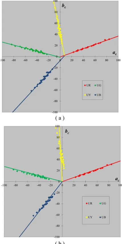
Fig. 2. The four NCS unique hue stimuli in the CIECAM02

ac–bc chromatic diagram: unique red (UR), unique yellow

(UY), unique green (UG) and unique blue (UB). (a) Best-fitting lines determined by orthogonal regression and (b) best-fitting lines with offset set to zero.

TABLE III. Values of the linear coefficients (K and C) and the associated perceptual errors for the four unique hue loci fitted for NCS data.

CIECAM02 fit

Unique red (UR)

Unique yellow (UY)

Unique green (UG)

Unique blue (UB)

K 0.37 25.26 20.27 1.13

C 20.54 41.29 21.24 27.14

DM represents colour difference units (DECAM02) and allows us to compare the goodness of fit for different unique hue datasets; it also allows us to evaluate whether an offset set to zero introduces a significant perceptual error.

To evaluate whether the fitted lines converge to the zero point statistically, we use a resampling method called ‘jack-knifing’16 on the distances from the origin to the most proximate point on the best-fitting line. The 95% confidence intervals for this distance measure are then calculated. If the line is statistically close to the ori-gin (i.e., if the distance between the oriori-gin and the most proximate point on the line is close to zero), then zero should be contained in the confidence interval.

Evaluation of the Default Unique Hues

In CIECAM02, four default hue angles are defined in ac–bcspace to represent the positions of the UR, UY, UG and UB loci, respectively. Two assumptions are made: (1) the hue angles are independent of both lightness and chroma, and (2) all unique hue lines pass through the ori-gin inac–bcspace, that is, the offset [C in Eq. (1)] is set to zero. The validity of the default unique hue lines (shown in Table II) is evaluated by comparing them with the hue angles derived from the NCS hues using Eq. (1).

Evaluation of Hue Uniformity

Hue uniformity is defined as the extent to which the perceived hue is independent of the two perceptual attrib-utes, lightness and chroma. As a measure of hue uniform-ity in CIECAM02, we used the average absolute perceptual hue differenceðjDHjÞ, which reflects the devi-ations of the individual hue angles at a particular chroma and lightness level from the grand mean:

DH52Cisin

hi2h

2

; (3)

where Ci and hi represent the chroma and hue angle of

theith unique hue stimulus, respectively, andh represents the mean hue angle (for red, green, yellow or blue). If the hue angle was completely independent of lightness and chroma, the average perceptual hue difference for each unique hue would be zero: increasing values of ðjDHjÞ indicate increasing deviations from hue uniformity.

Evaluation of Unique Hue Predictions for Different Media

A secondary aim of this study was to compare unique hue loci across different media. In our previous study,8 36 unique hue stimuli were assessed by 185 subjects on a calibrated CRT. The CRT display with a white point set at illuminant D93 and a neutral background was also set to have a chromaticity corresponding to D93. In contrast, the 108 NCS unique hue stimuli were painted physical samples that were seen by observers in a viewing cabinet with a light source representing a daylight simulator. To compare the unique hue loci across these two different media (self-luminous CRT stimuli vs. physical paint sam-ples), both sets of data were transformed to a common viewing condition in CIECAM02, the equi-energy illumi-nant (SE). This transformation takes into account the dif-ferent viewing conditions; the CIECAM02 input parameters for both datasets are listed in Table I. Note that for CRT unique hue, each of 185 observer data was adopted, whereas there is no observer data available for NCS unique hue.

RESULTS AND DISCUSSION

NCS Unique Hue Loci in CIECAM02

Colour appearance attributes for 108 NCS unique hue stimuli were predicted using CIECAM02. Figure 2 shows the distribution of unique hue stimuli in the CIECAM02 ac–bcchromatic diagram; each point in the diagram repre-sents a particular unique hue setting obtained in the origi-nal NCS experiment. In Fig. 2(a), the best-fitting line (using an orthogonal distance regression; see “Materials and Methods” section for details) is plotted for each unique hue. The estimated coefficients [K and C; see Eq. (1)] and the corresponding average errors [DM; see Eq. (2)] are given in Table III.

TABLE IV. Means and standard deviations of the

perceptual hue differences between individual

unique hues and average unique hue stimuli.

jDHj

Unique red (UR)

Unique yellow (UY)

Unique green (UG)

Unique blue (UB)

Mean 0.36 2.70 0.95 1.63

Standard deviation

0.41 2.22 0.67 1.08

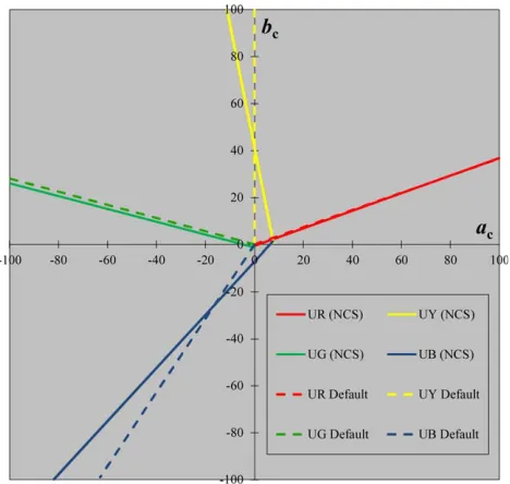
Fig. 3. The NCS unique hue (solid) lines and the CIE-CAM02 default unique hue (broken) lines in the CIECIE-CAM02

All perceptual errors (DM; Table III, row 3) are smaller or just about 1 DECAM02, indicating that the linear fit describes the data very well. The lines for UR and UG cross the b-axis at the points 20.54 and 21.24, respec-tively, and are reasonable close to the origin. For UY and UB, the estimated offsets are much larger (41.29 and 27.14).

The good linear fit of the NCS unique hue data is con-sistent with previous studies by Wuerger et al.,17 where unique hue data obtained on CRTs were fitted by a linear model in three-dimensional cone space or in a two-dimensional cone-opponent space (Derrington-Krauskopf-Lennie space18). The current study provides further evi-dence that unique hue loci can be modelled by straight lines in CIECAM02 and that there is no need to assume any nonlinearities, at least for the range of hues produced

on CRTs and for the physical samples used in the NCS study.

Figure 2(b) shows the best-fitting line when the unique hue lines are constrained to pass through the origin of the CIECAM02 ac–bc chromatic diagram [offset C50; Fig. 2(b)]. An offset fixed at zero results in a poor fit of the linear model as demonstrated by the increase in the per-ceptual error (DM; last row of Table III). For UY, the error rises by a factor of 3; for the other hues, the error increases by at least 50%.

Comparison of the NCS Unique Hue Loci with the Default Unique Hue Loci

In Fig. 3, the predicted NCS unique hue loci with the default unique hue loci in CIECAM02 ac–bc chromatic

diagram is compared, where the solid lines represent the NCS unique hue lines, and the broken lines represent the default unique hue loci in CIECAM02. There is overall good agreement for UR and UG; however, there were clear discrepancies for both the UY and UB lines. The UB and UY lines are not consistent with an offset of zero, which is assumed for the default unique hue lines.

This discrepancy between the unique hue prediction and the default unique hue lines has been reported previ-ously by Kuehni and coworkers. Hinks et al.19reported a study to assess the unique hue stimuli using the samples from the Munsell Book of Color. As summarized by Kuehni et al.,20 they found that when these unique hue loci were transformed to CIECAM02, there were clear discrepancies between the predicted unique hue loci and the default unique hue loci. These studies used a different methodology to obtain the unique hue lines, but arrived at the same conclusions as our current analysis.

Evaluation of Hue Uniformity

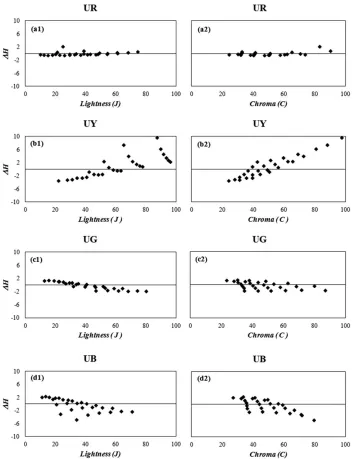
To evaluate hue uniformity, the absolute mean value and the standard deviation of the perceptual hue differen-ces were calculated for each unique hue using Eq. (3), and the results are shown in Table IV. The average per-ceptual hue difference was less than unity for both UR (0.36) and UG (0.95) demonstrating fairly good hue uni-formity. The hue uniformity for both UY and UB is worse: their mean perceptual hue differences were 2.70 and 1.63, respectively.

To investigate the factors causing the violation of hue uniformity, the perceptual hue difference is plotted as a function of lightness (left panels in Fig. 4) or the chroma attribute (right panel in Fig. 4). The four rows (a–d) in Fig. 4 represent the four unique hues, UR, UY, UG and UB, respectively. For each subfigure, the individual points

represent a NCS unique hue stimulus in CIECAM02. The ordinate represents the perceptual hue difference between each individual unique hue stimulus and the average unique hue stimuli; the abscissa represents either the lightness (left) or the chroma (right) attribute for the cor-responding unique hue stimulus.

Hue uniformity for UR (Fig. 4, row 1) is fairly good that most of the hue differences are very small, less than 0.5, indicating that there is only a small hue shift for the UR stimuli with changes of either lightness or chroma attributes. For UY (Fig. 4, row 2), an increase of either the lightness or the chroma attribute leads to large changes in the perceptual hue differences change system-atically from 24 to 110 units; hue values need to be increased to achieve a constant perceptual UY. For UG (Fig. 4, row 3), an increase in lightness results in percep-tual hue difference changes from 12 to 22, implying that the hue value needs to decrease to preserve a con-stant perceptual hue. When chroma increases, the same trends in the hue shift can be found; however, there was a large scatter between the hues. For UB (Fig. 4, row 4), the hue value in CIECAM02 needs to be decreased to perceive a UB when the lightness or chroma attributes increase.

Fig. 5. Ebner and Fairchild’s constant hue data in the CIECAM02ac–bcchromatic diagram.

Fig. 6. Comparison between CRT unique hue stimuli and NCS unique hue stimuli in CIECAM02 ac–bc chromatic

diagram.

TABLE V. Values of the linear coefficients (K and C) and the associated perceptual errors for the four unique hue loci fitted for CRT data.

CIECAM02 fit

Unique red (UR)

Unique yellow (UY)

Unique green (UG)

Unique blue (UB)

K 0.32 29.68 20.43 1.02

C 22.34 46.77 23.72 29.20

These changes in hue with changes in lightness and chroma could cause detrimental performance for colour reproduction processes that are required to preserve hue, such as brightness enhancement or saturation enhance-ment. Moreover, systematic hue shifts in UY and UB could enhance this effect as a larger lightness or chroma causes a larger perceived hue shift.

The poor performance of hue uniformity for UY and UB might be caused by the fact that the intersection of the UY locus and the UB locus is not close to the origin, the neutral point, in the CIECAM02ac–bcchromatic dia-gram. This also suggests how CIECAM02 might be modi-fied to improve its hue uniformity.

Ebner and Fairchild21 derived a set of constant hue data on a CRT display, where 30 observers were asked to choose a set of colour patches that had the same hue at different lightness and chroma levels. Observers selected 20–25 patches for each of 15 hues, and their CIE XYZ tristimulus values were recorded. These constant hue data were transformed to CIECAM02 using the input parame-ters given in the third row of Table I. Figure 5 illustrates all these constant hue data (solid symbols) in CIECAM02 chromatic space and compares them with proposed unique hue loci (solid lines). UR, UY and UG loci all correspond well with the constant hue data of Hue 2, Hue 5 and Hue 8, indicating the same problem of hue uni-formity as discussed above. There is some disagreement between the UB loci and the Hue 12 data for samples with high chroma.

Unique Hue Loci for Different Media

To compare the unique hue loci between the CRT data8and NCS data, we plotted both datasets in the same CIECAM02 ac–bc chromatic diagram (Fig. 6). For UY and UB, the NCS data (open red diamonds) and the CRT data (closed blue triangles) are virtually indistinguishable, and the NCS settings are within measurement error of the CRT data. For UR and UG, there are systematic devia-tions between the CRT and the NCS data, in particular at higher chroma values.

As for the NCS data, we used orthogonal distance regression to estimate the slopes and offsets of the best-fitting lines for the CRT data (Table V). The perceptual error under the linear model with and without offset (C50) was calculated and given in the last two row of Table V. As expected, the model fit is always better when the additional parameter (offset) is allowed to vary. The largest improvement occurs for UY, consistent with the NCS analysis (Table III). In Fig. 6, the best-fitting

lines for both the CRT unique hue stimuli (solid lines) and the NCS unique hue stimuli (dashed lines) are plotted in the CIECAM02ac–bcchromatic diagram.

To evaluate whether the best-fitting regression lines for both datasets (NCS and CRT) converge to zero, we used a data resampling method (see “Materials and Methods” sec-tion). Specifically, we test whether the distance between the origin and the most proximate point on the fitted line is stat-istically different from zero, by calculating the upper and lower 95% confidence intervals for this distance measure. Table VI shows the average distance from the origin, together with the 95% confidence intervals, for both the NCS and the CRT dataset. In accordance with Fig. 6, the convergence for UR and UG is generally better than for UY and UB. For the NCS data (dashed lines), the zero point is—for all practical purposes—contained in the 95% confidence limits (Table VI, row 1); for the CRT data (solid lines), the lines do not converge to the origin, and this devi-ation is outside of the 95% confidence intervals in both cases (Table VI, row 2). For UY and UB, both datasets show the same effect (Fig. 6), and in both cases, the lines do not converge to the origin, that is, zero is not contained in the 95% confidence interval (Table VI, rows 1 and 2).

The systematic deviations from the default unique hue lines (Fig. 3) are common for both datasets. Both datasets demonstrate that when converted to CIECAM02, the unique hue lines do not converge to the zero point (Fig. 6; cf. Table VI). This systematic error is more pronounced for UY and UB, but reaches statistical significance for UR and UG in the CRT datasets.

Keeping in mind that these two sets of unique hue loci were derived using different media (CRT vs. physical samples), different viewing conditions and different sets of observers, their appearance attributes in CIECAM02 are in reasonably good agreement. This suggests that the chromatic adaptation transform used in the CIECAM02 model captures some important aspects of colour appear-ance changes under different viewing conditions.

CONCLUSIONS

The NCS unique hue data were used to evaluate the qual-ity of the unique hue predictions and hue uniformqual-ity in the CIECAM02 colour appearance model. Colour appear-ance attributes were predicted using the original viewing conditions under which the data were collected. Subse-quently, the loci of unique hue data in the CIECAM02 ac–bc chromatic diagram were compared with the default unique hue lines. Our main conclusions are as follows:

TABLE VI. Distances of the best-fitting hue line from the origin (do) with upper and lower 95% confidence limits.

do

Unique red (UR)

Unique yellow (UY)

Unique green (UG)

Unique blue (UB)

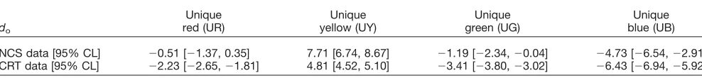
NCS data [95% CL] 20.51 [21.37, 0.35] 7.71 [6.74, 8.67] 21.19 [22.34,20.04] 24.73 [26.54,22.91]

1. We found a clear discrepancy between the NCS and the default unique hue loci for UY and UB; the unique hue lines do not converge to the zero point in the CIE-CAM02ac–bcchromatic diagram.

2. Hue uniformity in CIECAM02 was evaluated by calcu-lating the perceptual hue differences at different light-ness and chroma levels. Systematic hue shifts were found for UY and UB. When lightness or chroma attrib-utes are increased, hue values in CIECAM02 needed to be increased to preserve a UY locus and needed to be decreased to preserve a UB locus. Approximate hue uni-formity holds for UR.

3. Media differences that might affect unique hue predic-tions were investigated by comparing NCS (physical samples) and CRT unique hue data (self-luminous stim-uli); these two datasets agree reasonably well in CIE-CAM02, suggesting that the chromatic adaptation transform used in CIECAM02 captures some important aspects of visual adaptation mechanisms.

1. CIE Publication 159:2004. A Color Appearance Model for Color Man-agement Systems. Vienna, Austria: CIE Central Bureau; 2004. 2. Fairchild MD. Color Appearance Models, 2nd edition. Reading: Wiley;

2005.

3. Luo MR, Hunt RWG. The structure of the CIE 1997 Colour Appear-ance Model (CIECAM97s). Color Res Appl 1998;23:138–146. 4. Hering E. Outlines of a Theory of the Light Sense [Translated by L. M.

Hurvich and D. Jameson]. Cambridge: Harvard University Press; 1964. 5. Ha˚rd A, Sivik L, Tonnquist G. NCS, Natural color system—From

con-cept to research and application, Part I. Color Res Appl 1996;21:180– 205.

6. Hunt RWG. A model of colour vision for predicting colour appearance. Color Res Appl 1982;7:95–112.

7. Hunt RWG, Pointer MR. Measuring colour, 4th edition. Winchester, UK: Wiley; 2011.

8. Xiao K, Wuerger S, Fu C, Karatzas D. Unique hue data for colour appearance models. Part I: Loci of unique hues and hue uniformity. Color Res Appl 2011;36:316–323.

9. Xiao K, Fu C, Maylons D, Karatzas D, Wuerger S. Unique hue data for colour appearance models. Part II: Chromatic adaptation transform. Color Res Appl 2013;38:22229.

10. Wuerger S, Xiao K, Fu C, Karatzas D. Colour-opponent mechanisms are not affected by sensitivity changes with ageing. Ophthalmic Physiol Opt 2010;30:653–659.

11. Fu C, Xiao K, Karatzas D, Wuerger SM. Investigation of unique hue setting changes with ageing. Chin Opt Lett 2011;9:053301.1-5. 12. Swedish Standard SS 01 91 03. Tristimulus values and chromaticity

coordinates for the color samples in SS 01 91 02. Stockholm: Swedish Standards Institute; 1982.

13. Jobson JD. Applied Multivariate Data Analysis, Vols. 1 and 2. New York: Springer; 1991.

14. Luo MR, Cui G, Li C. Uniform colour spaces based on CIECAM02 colour appearance model. Color Res Appl 2006;31:320–330.

15. Ballantine JP, Jerbert AR. Distance from a line or plane to a point. Am Math Mon 1952;59:242–243.

16. Shao J, Wu CFJ. A general theory for Jack-knife variance estimation. Ann Stat 1989;17:1176–1197.

17. Wuerger SM, Atkinson P, Cropper S. The cone inputs to the unique-hue mechanisms. Vision Res 2005;45:3210–3223.

18. Derrington AM, Krauskopf J, Lennie P. Chromatic mechanisms in lat-eral geniculate nucleus of macaque. J Physiol 1984;357:241–265. 19. Hinks D, Cardenas LM, Kuehni RG, Shamey R. Unique-hue stimulus

selection using Munsell color chips. J Opt Soc A 2007;24:3371–3378. 20. Kuehni RG, Hinks D, Shamey R. Experimental object color unique hue

data for the mean observer for color appearance modelling. Color Res Appl 2008;33:505–506.