Feature Extraction
and
Dedication
Feature Extraction
and
Image Processing
Mark S. Nixon
Alberto S. Aguado
Newnes
Newnes
An imprint of Butterworth-Heinemann Linacre House, Jordan Hill, Oxford OX2 8DP 225 Wildwood Avenue, Woburn, MA 01801-2041
A division of Reed Educational and Professional Publishing Ltd
A member of the Reed Elsevier plc group
First edition 2002
© Mark S. Nixon and Alberto S. Aguado 2002
All rights reserved. No part of this publication may be reproduced in any material form (including photocopying or storing in any medium by electronic means and whether or not transiently or incidentally to some other use of this publication) without the written permission of the copyright holder except in accordance with the provisions of the Copyright, Designs and Patents Act 1988 or under the terms of a licence issued by the Copyright Licensing Agency Ltd, 90 Tottenham Court Road, London, England W1P 0LP. Applications for the copyright holder’s written permission to reproduce any part of this publication should be addressed to the publishers
British Library Cataloguing in Publication Data
A catalogue record for this book is available from the British Library
ISBN 0 7506 5078 8
Preface
...
ix
Why did we write this book?
...
ix
The book and its support
...
x
In gratitude
...
xii
Final message
...
xii
1 Introduction
...
1
1.1 Overview
...
1
1.2 Human and computer vision
...
1
1.3 The human vision system
...
3
1.4 Computer vision systems
...
10
1.5 Mathematical systems
...
15
1.6 Associated literature
...
24
1.7 References
...
28
2 Images, sampling and frequency domain
processing
...
31
2.1 Overview
...
31
2.2 Image formation
...
31
2.3 The Fourier transform
...
35
2.4 The sampling criterion
...
40
2.5 The discrete Fourier transform ( DFT)
...
45
2.6 Other properties of the Fourier transform
...
53
2.7 Transforms other than Fourier
...
57
2.8 Applications using frequency domain properties
....
63
2.9 Further reading
...
65
2.10 References
...
65
3 Basic image processing operations
...
67
3.1 Overview
...
67
3.2 Histograms
...
67
3.3 Point operators
...
69
3.4 Group operations
...
79
3.5 Other statistical operators
...
88
3.6 Further reading
...
95
4 Low- level feature extraction ( including edge
detection)
...
99
4.1 Overview
...
99
4.2 First-order edge detection operators
...
99
4.3 Second- order edge detection operators
...
120
4.4 Other edge detection operators
...
127
4.5 Comparison of edge detection operators
...
129
4.6 Detecting image curvature
...
130
4.7 Describing image motion
...
145
4.8 Further reading
...
156
4.9 References
...
157
5 Feature extraction by shape matching
...
161
5.1 Overview
...
161
5.2 Thresholding and subtraction
...
162
5.3 Template matching
...
164
5.4 Hough transform (HT)
...
173
5.5 Generalised Hough transform (GHT)
...
199
5.6 Other extensions to the HT
...
213
5.7 Further reading
...
214
5.8 References
...
214
6 Flexible shape extraction ( snakes and other
techniques)
...
217
6.1 Overview
...
217
6.2 Deformable templates
...
218
6.3 Active contours (snakes)
...
220
6.4 Discrete symmetry operator
...
236
6.5 Flexible shape models
...
240
6.6 Further reading
...
243
6.7 References
...
243
7 Object description
...
247
7.1 Overview
...
247
7.2 Boundary descriptions
...
248
7.3 Region descriptors
...
278
7.5 References
...
288
8 Introduction to texture description,
segmentation and classification
...
291
8.1 Overview
...
291
8.2 What is texture?
...
292
8.3 Texture description
...
294
8.4 Classification
...
301
8.5 Segmentation
...
306
8.6 Further reading
...
307
8.7 References
...
308
Appendices
...
311
9.1 Appendix 1: Homogeneous co-ordinate system
...
311
9.2 Appendix 2: Least squares analysis
...
314
9.3 Appendix 3: Example Mathcad worksheet for
Chapter 3
...
317
9.4 Appendix 4: Abbreviated Matlab worksheet
...
336
Preface
Why did we write this book?
We will no doubt be asked many times: why on earth write a new book on computer vision? Fair question: there are already many good books on computer vision already out in the bookshops, as you will find referenced later, so why add to them? Part of the answer is that any textbook is a snapshot of material that exists prior to it. Computer vision, the art of processing images stored within a computer, has seen a considerable amount of research by highly qualified people and the volume of research would appear to have increased in recent years. That means a lot of new techniques have been developed, and many of the more recent approaches have yet to migrate to textbooks.
But it is not just the new research: part of the speedy advance in computer vision technique has left some areas covered only in scant detail. By the nature of research, one cannot publish material on technique that is seen more to fill historical gaps, rather than to advance knowledge. This is again where a new text can contribute.
Finally, the technology itself continues to advance. This means that there is new hardware, new programming languages and new programming environments. In particular for computer vision, the advance of technology means that computing power and memory are now relatively cheap. It is certainly considerably cheaper than when computer vision was starting as a research field. One of the authors here notes that the laptop that his portion of the book was written on has more memory, is faster, has bigger disk space and better graphics than the computer that served the entire university of his student days. And he is not that old! One of the more advantageous recent changes brought by progress has been the development of mathematical programming systems. These allow us to concentrate on mathematical technique itself, rather than on implementation detail. There are several sophisticated flavours of which Mathcad and Matlab, the chosen vehicles here, are amongst the most popular. We have been using these techniques in research and in teaching and we would argue that they have been of considerable benefit there. In research, they help us to develop technique faster and to evaluate its final implementation. For teaching, the power of a modern laptop and a mathematical system combine to show students, in lectures and in study, not only how techniques are implemented, but also how and why they work with an explicit relation to conventional teaching material.
The book and its support
Each chapter of the book presents a particular package of information concerning feature extraction in image processing and computer vision. Each package is developed from its origins and later referenced to more recent material. Naturally, there is often theoretical development prior to implementation (in Mathcad or Matlab). We have provided working implementations of most of the major techniques we describe, and applied them to process a selection of imagery. Though the focus of our work has been more in analysing medical imagery or in biometrics (the science of recognising people by behavioural or physiological characteristic, like face recognition), the techniques are general and can migrate to other application domains.
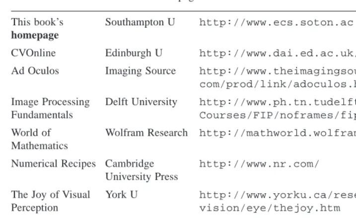
You will find a host of further supporting information at the book’s website http://
www.ecs.soton.ac.uk/~msn/book/.First, you will find the worksheets (the Matlab
and Mathcad implementations that support the text) so that you can study the techniques described herein. There are also lecturing versions that have been arranged for display via a data projector, with enlarged text and more interactive demonstration. The website will be kept as up to date as possible, for it also contains links to other material such as websites devoted to techniques and to applications, as well as to available software and on-line literature. Finally, any errata will be reported there. It is our regret and our responsibility that these will exist, but our inducement for their reporting concerns a pint of beer. If you find an error that we don’t know about (not typos like spelling, grammar and layout) then use the mailto on the website and we shall send you a pint of good English beer, free!
There is a certain amount of mathematics in this book. The target audience is for third or fourth year students in BSc/BEng/MEng courses in electrical or electronic engineering, or in mathematics or physics, and this is the level of mathematical analysis here. Computer vision can be thought of as a branch of applied mathematics, though this does not really apply to some areas within its remit, but certainly applies to the material herein. The mathematics essentially concerns mainly calculus and geometry though some of it is rather more detailed than the constraints of a conventional lecture course might allow. Certainly, not all the material here is covered in detail in undergraduate courses at Southampton.
The book starts with an overview of computer vision hardware, software and established material, with reference to the most sophisticated vision system yet ‘developed’: the human
vision system. Though the precise details of the nature of processing that allows us to see
have yet to be determined, there is a considerable range of hardware and software that allow us to give a computer system the capability to acquire, process and reason with imagery, the function of ‘sight’. The first chapter also provides a comprehensive bibliography of material you can find on the subject, not only including textbooks, but also available software and other material. As this will no doubt be subject to change, it might well be worth consulting the website for more up-to-date information. The preference for journal references are those which are likely to be found in local university libraries, IEEE
Transactions in particular. These are often subscribed to as they are relatively low cost, and
are often of very high quality.
equations, but it is a new way of looking at data and at signals, and proves to be a rewarding topic of study in its own right.
We then start to look at basic image processing techniques, where image points are mapped into a new value first by considering a single point in an original image, and then by considering groups of points. Not only do we see common operations to make a picture’s appearance better, especially for human vision, but also we see how to reduce the effects of different types of commonly encountered image noise. This is where the techniques are implemented as algorithms in Mathcad and Matlab to show precisely how the equations work.
The following chapter concerns low-level features which are the techniques that describe the content of an image, at the level of a whole image rather than in distinct regions of it. One of the most important processes we shall meet is called edge detection. Essentially, this reduces an image to a form of a caricaturist’s sketch, though without a caricaturist’s exaggerations. The major techniques are presented in detail, together with descriptions of their implementation. Other image properties we can derive include measures of curvature and measures of movement. These also are covered in this chapter.
These edges, the curvature or the motion need to be grouped in some way so that we can find shapes in an image. Our first approach to shape extraction concerns analysing the
match of low-level information to a known template of a target shape. As this can be
computationally very cumbersome, we then progress to a technique that improves computational performance, whilst maintaining an optimal performance. The technique is known as the Hough transform and it has long been a popular target for researchers in computer vision who have sought to clarify its basis, improve it speed, and to increase its accuracy and robustness. Essentially, by the Hough transform we estimate the parameters that govern a shape’s appearance, where the shapes range from lines to ellipses and even to unknown shapes.
Some applications of shape extraction require to determine rather more than the parameters that control appearance, but require to be able to deform or flex to match the image template. For this reason, the chapter on shape extraction by matching is followed by one on flexible shape analysis. This is a topic that has shown considerable progress of late, especially with the introduction of snakes (active contours). These seek to match a shape to an image by analysing local properties. Further, we shall see how we can describe a shape by its symmetry and also how global constraints concerning the statistics of a shape’s appearance can be used to guide final extraction.
Up to this point, we have not considered techniques that can be used to describe the shape found in an image. We shall find that the two major approaches concern techniques that describe a shape’s perimeter and those that describe its area. Some of the perimeter
description techniques, the Fourier descriptors, are even couched using Fourier transform
theory that allows analysis of their frequency content. One of the major approaches to area
description, statistical moments, also has a form of access to frequency components, but is
of a very different nature to the Fourier analysis.
The final chapter describes texture analysis, prior to some introductory material on
pattern classification. Texture describes patterns with no known analytical description and
The appendices include material that is germane to the text, such as co-ordinate geometry and the method of least squares, aimed to be a short introduction for the reader. Other related material is referenced throughout the text, especially to on-line material. The appendices include a printout of one of the shortest of the Mathcad and Matlab worksheets.
In this way, the text covers all major areas of feature extraction in image processing and computer vision. There is considerably more material in the subject than is presented here: for example, there is an enormous volume of material in 3D computer vision and in 2D signal processing which is only alluded to here. But to include all that would lead to a monstrous book that no one could afford, or even pick up! So we admit we give a snapshot, but hope more that it is considered to open another window on a fascinating and rewarding subject.
In gratitude
We are immensely grateful to the input of our colleagues, in particular to Dr Steve Gunn and to Dr John Carter. The family who put up with it are Maria Eugenia and Caz and the nippers. We are also very grateful to past and present researchers in computer vision at the Image, Speech and Intelligent Systems Research Group (formerly the Vision, Speech and Signal Processing Group) under (or who have survived?) Mark’s supervision at the Department of Electronics and Computer Science, University of Southampton. These include: Dr Hani Muammar, Dr Xiaoguang Jia, Dr Yan Chen, Dr Adrian Evans, Dr Colin Davies, Dr David Cunado, Dr Jason Nash, Dr Ping Huang, Dr Liang Ng, Dr Hugh Lewis, Dr David Benn, Dr Douglas Bradshaw, David Hurley, Mike Grant, Bob Roddis, Karl Sharman, Jamie Shutler, Jun Chen, Andy Tatem, Chew Yam, James Hayfron-Acquah, Yalin Zheng and Jeff Foster. We are also very grateful to past Southampton students on BEng and MEng Electronic Engineering, MEng Information Engineering, BEng and MEng Computer Engineering and BSc Computer Science who have pointed out our earlier mistakes, noted areas for clarification and in some cases volunteered some of the material herein. To all of you, our very grateful thanks.
Final message
We ourselves have already benefited much by writing this book. As we already know, previous students have also benefited, and contributed to it as well. But it remains our hope that it does inspire people to join in this fascinating and rewarding subject that has proved to be such a source of pleasure and inspiration to its many workers.
Mark S. Nixon Alberto S. Aguado
1
Introduction
1.1 Overview
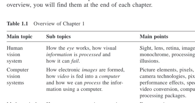
[image:12.595.51.447.292.502.2]This is where we start, by looking at the human visual system to investigate what is meant by vision, then on to how a computer can be made to sense pictorial data and then how we can process it. The overview of this chapter is shown in Table 1.1; you will find a similar overview at the start of each chapter. We have not included the references (citations) in any overview, you will find them at the end of each chapter.
Table 1.1 Overview of Chapter 1
Main topic Sub topics Main points
Human How the eye works, how visual Sight, lens, retina, image, colour, vision information is processed and monochrome, processing, brain,
system how it can fail. illusions.
Computer How electronic images are formed, Picture elements, pixels, video standard, vision how video is fed into a computer camera technologies, pixel technology, systems and how we can process the infor- performance effects, specialist cameras,
mation using a computer. video conversion, computer languages, processing packages.
Mathematical How we can process images using Ease, consistency, support, visualisation systems mathematical packages; intro- of results, availability, introductory use,
duction to the Matlab and Mathcad example worksheets. systems.
Literature Other textbooks and other places to Magazines, textbooks, websites and find information on image proces- this book’s website.
sing, computer vision and feature extraction.
1.2 Human and computer vision
computer vision techniques. Forensic studies and biometrics (ways to recognise people) using computer vision include automatic face recognition and recognising people by the ‘texture’ of their irises. These studies are paralleled by biologists and psychologists who continue to study how our human vision system works, and how we see and recognise objects (and people).
A selection of (computer) images is given in Figure 1.1, these images comprise a set of points or picture elements (usually concatenated to pixels) stored as an array of numbers in a computer. To recognise faces, based on an image such as Figure 1.1(a), we need to be able to analyse constituent shapes, such as the shape of the nose, the eyes, and the eyebrows, to make some measurements to describe, and then recognise, a face. (Figure 1.1(a) is perhaps one of the most famous images in image processing. It is called the Lena image, and is derived from a picture of Lena Sjööblom in Playboy in 1972.) Figure 1.1(b) is an ultrasound image of the carotid artery (which is near the side of the neck and supplies blood to the brain and the face), taken as a cross-section through it. The top region of the image is near the skin; the bottom is inside the neck. The image arises from combinations of the reflections of the ultrasound radiation by tissue. This image comes from a study aimed to produce three-dimensional models of arteries, to aid vascular surgery. Note that the image is very noisy, and this obscures the shape of the (elliptical) artery. Remotely sensed images are often analysed by their texture content. The perceived texture is different between the road junction and the different types of foliage seen in Figure 1.1(c). Finally, Figure 1.1(d) is a Magnetic Resonance Image (MRI) of a cross-section near the middle of a human body. The chest is at the top of the image, and the lungs and blood vessels are the dark areas, the internal organs and the fat appear grey. MRI images are in routine medical use nowadays, owing to their ability to provide high quality images.
Figure 1.1 Real images from different sources
There are many different image sources. In medical studies, MRI is good for imaging soft tissue, but does not reveal the bone structure (the spine cannot be seen in Figure 1.1(d)); this can be achieved by using Computerised Tomography (CT) which is better at imaging bone, as opposed to soft tissue. Remotely sensed images can be derived from infrared (thermal) sensors or Synthetic-Aperture Radar, rather than by cameras, as in Figure 1.1(c). Spatial information can be provided by two-dimensional arrays of sensors, including sonar arrays. There are perhaps more varieties of sources of spatial data in medical studies than in any other area. But computer vision techniques are used to analyse any form of data, not just the images from cameras.
Synthesised images are good for evaluating techniques and finding out how they work,
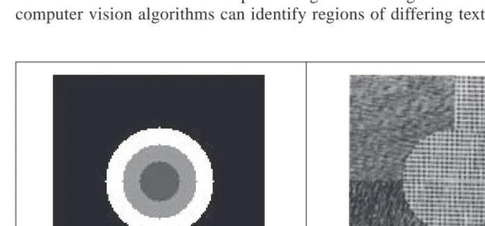
[image:14.595.53.404.199.363.2]and some of the bounds on performance. Two synthetic images are shown in Figure 1.2. Figure 1.2(a) is an image of circles that were specified mathematically. The image is an ideal case: the circles are perfectly defined and the brightness levels have been specified to be constant. This type of synthetic image is good for evaluating techniques which find the borders of the shape (its edges), the shape itself and even for making a description of the shape. Figure 1.2(b) is a synthetic image made up of sections of real image data. The borders between the regions of image data are exact, again specified by a program. The image data comes from a well-known texture database, the Brodatz album of textures. This was scanned and stored as computer images. This image can be used to analyse how well computer vision algorithms can identify regions of differing texture.
Figure 1.2 Examples of synthesised images
(a) Circles (b) Textures
This chapter will show you how basic computer vision systems work, in the context of the human vision system. It covers the main elements of human vision showing you how your eyes work (and how they can be deceived!). For computer vision, this chapter covers the hardware and software used for image analysis, giving an introduction to Mathcad and Matlab, the software tools used throughout this text to implement computer vision algorithms. Finally, a selection of pointers to other material is provided, especially those for more detail on the topics covered in this chapter.
1.3 The human vision system
Human vision is a sophisticated system that senses and acts on visual stimuli. It has evolved for millions of years, primarily for defence or survival. Intuitively, computer and human vision appear to have the same function. The purpose of both systems is to interpret
spatial data, data that is indexed by more than one dimension. Even though computer and
useful when developing computer vision techniques, whereas others are actually undesirable in a computer vision system. But we shall see computer vision techniques which can to some extent replicate, and in some cases even improve upon, the human vision system.
You might ponder this, so put one of the fingers from each of your hands in front of your face and try to estimate the distance between them. This is difficult, and we are sure you would agree that your measurement would not be very accurate. Now put your fingers very close together. You can still tell that they are apart even when the distance between them is tiny. So human vision can distinguish relative distance well, but is poor for absolute distance. Computer vision is the other way around: it is good for estimating absolute difference, but with relatively poor resolution for relative difference. The number of pixels in the image imposes the accuracy of the computer vision system, but that does not come until the next chapter. Let us start at the beginning, by seeing how the human vision system works.
In human vision, the sensing element is the eye from which images are transmitted via the optic nerve to the brain, for further processing. The optic nerve has insufficient capacity to carry all the information sensed by the eye. Accordingly, there must be some pre-processing before the image is transmitted down the optic nerve. The human vision system can be modelled in three parts:
1. the eye − this is a physical model since much of its function can be determined by pathology;
2. the neural system − this is an experimental model since the function can be modelled, but not determined precisely;
3. processing by the brain − this is a psychological model since we cannot access or model such processing directly, but only determine behaviour by experiment and inference.
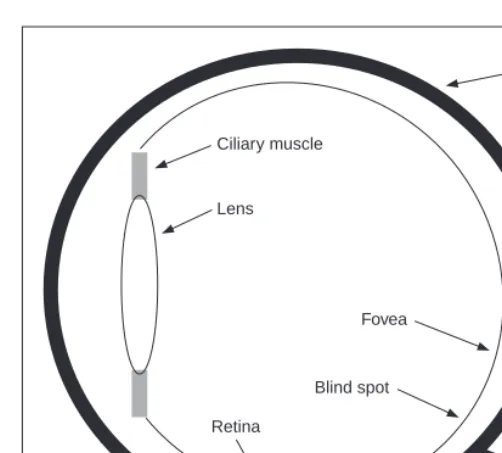
1.3.1 The eye
The function of the eye is to form an image; a cross-section of the eye is illustrated in Figure 1.3. Vision requires an ability to focus selectively on objects of interest. This is achieved by the ciliary muscles that hold the lens. In old age, it is these muscles which become slack and the eye loses its ability to focus at short distance. The iris, or pupil, is like an aperture on a camera and controls the amount of light entering the eye. It is a delicate system and needs protection, this is provided by the cornea (sclera). The choroid has blood vessels that supply nutrition and is opaque to cut down the amount of light. The
retina is on the inside of the eye, which is where light falls to form an image. By this
system, muscles rotate the eye, and shape the lens, to form an image on the fovea (focal point) where the majority of sensors are situated. The blind spot is where the optic nerve starts; there are no sensors there.
Focusing involves shaping the lens, rather than positioning it as in a camera. The lens is shaped to refract close images greatly, and distant objects little, essentially by ‘stretching’ it. The distance of the focal centre of the lens varies from approximately 14 mm to around 17 mm depending on the lens shape. This implies that a world scene is translated into an area of about 2 mm2. Good vision has high acuity (sharpness), which implies that there must be very many sensors in the area where the image is formed.
Ciliary muscle
Choroid
Lens
Retina
Blind spot Fovea
Optic nerve
these sensors to stimulate photochemical transmissions, which results in nerve impulses that are collected to form the signal transmitted by the eye. There are two types of sensor: first, the rods−these are used for black and white (scotopic) vision; and secondly, the
cones –these are used for colour (photopic) vision. There are approximately 10 million
cones and nearly all are found within 5° of the fovea. The remaining 100 million rods are distributed around the retina, with the majority between 20°and 5°of the fovea. Acuity is actually expressed in terms of spatial resolution (sharpness) and brightness/colour resolution, and is greatest within 1° of the fovea.
There is only one type of rod, but there are three types of cones. These types are:
1. α − these sense light towards the blue end of the visual spectrum;
2. β − these sense green light;
3. γ − these sense light in the red region of the spectrum.
The total response of the cones arises from summing the response of these three types of cones, this gives a response covering the whole of the visual spectrum. The rods are sensitive to light within the entire visual spectrum, and are more sensitive than the cones. Accordingly, when the light level is low, images are formed away from the fovea, to use the superior sensitivity of the rods, but without the colour vision of the cones. Note that there are actually very few of the α cones, and there are many more β and γ cones. But we can still see a lot of blue (especially given ubiquitous denim!). So, somehow, the human vision system compensates for the lack of blue sensors, to enable us to perceive it. The world would be a funny place with red water! The vision response is actually logarithmic and depends on brightness adaption from dark conditions where the image is formed on the rods, to brighter conditions where images are formed on the cones.
[image:16.595.54.305.45.271.2](a) Image showing the Mach band effect
mach0,x 100 200
0 50 100
x
(b) Cross-section through (a)
seenx 100 200
0 50 100
x
(c) Perceived cross-section through (a)
[image:17.595.55.399.257.554.2]images. These are illustrated in Figure 1.4 and are the darker bands that appear to be where two stripes of constant shade join. By assigning values to the image brightness levels, the cross-section of plotted brightness is shown in Figure 1.4(a). This shows that the picture is formed from stripes of constant brightness. Human vision perceives an image for which the cross-section is as plotted in Figure 1.4(c). These Mach bands do not really exist, but are introduced by your eye. The bands arise from overshoot in the eyes’ response at boundaries of regions of different intensity (this aids us to differentiate between objects in our field of view). The real cross-section is illustrated in Figure 1.4(b). Note also that a human eye can distinguish only relatively few grey levels. It actually has a capability to discriminate between 32 levels (equivalent to five bits) whereas the image of Figure 1.4(a) could have many more brightness levels. This is why your perception finds it more difficult to discriminate between the low intensity bands on the left of Figure 1.4(a). (Note that that Mach bands cannot be seen in the earlier image of circles, Figure 1.2(a), due to the arrangement of grey levels.) This is the limit of our studies of the first level of human vision; for those who are interested, Cornsweet (1970) provides many more details concerning visual perception.
Figure 1.4 Illustrating the Mach band effect
bands and sensitivity to unsensed phenomena. These properties are integral to human vision. At present, human vision is far more sophisticated than we can hope to achieve with a computer vision system. Infrared guided-missile vision systems can actually have difficulty in distinguishing between a bird at 100 m and a plane at 10 km. Poor birds! (Lucky plane?) Human vision can handle this with ease.
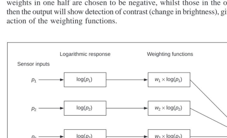
1.3.2 The neural system
Neural signals provided by the eye are essentially the transformed response of the wavelength dependent receptors, the cones and the rods. One model is to combine these transformed signals by addition, as illustrated in Figure 1.5. The response is transformed by a logarithmic function, mirroring the known response of the eye. This is then multiplied by a weighting factor that controls the contribution of a particular sensor. This can be arranged to allow a combination of responses from a particular region. The weighting factors can be chosen to afford particular filtering properties. For example, in lateral inhibition, the weights for the centre sensors are much greater than the weights for those at the extreme. This allows the response of the centre sensors to dominate the combined response given by addition. If the weights in one half are chosen to be negative, whilst those in the other half are positive, then the output will show detection of contrast (change in brightness), given by the differencing action of the weighting functions.
p1
p2
p3
p4
p5
log(p1)
log(p2)
log(p3)
log(p4)
log(p5)
w1× log(p1)
w2× log(p2)
w3× log(p3)
w4× log(p4)
w5× log(p5)
Output ∑
Sensor inputs
[image:18.595.54.419.311.532.2]Logarithmic response Weighting functions
Figure 1.5 Neural processing
sensors are combined prior to transmission through the optic nerve. This is an experimental model, since there are many ways possible to combine the different signals together. For further information on retinal neural networks, see Ratliff (1965); an alternative study of neural processing can be found in Overington (1992).
1.3.3 Processing
The neural signals are then transmitted to two areas of the brain for further processing. These areas are the associative cortex, where links between objects are made, and the
occipital cortex, where patterns are processed. It is naturally difficult to determine precisely
what happens in this region of the brain. To date, there have been no volunteers for detailed study of their brain’s function (though progress with new imaging modalities such as Positive Emission Tomography or Electrical Impedance Tomography will doubtless help). For this reason, there are only psychological models to suggest how this region of the brain operates.
It is well known that one function of the eye is to use edges, or boundaries, of objects. We can easily read the word in Figure 1.6(a), this is achieved by filling in the missing boundaries in the knowledge that the pattern most likely represents a printed word. But we can infer more about this image; there is a suggestion of illumination, causing shadows to appear in unlit areas. If the light source is bright, then the image will be washed out, causing the disappearance of the boundaries which are interpolated by our eyes. So there is more than just physical response, there is also knowledge, including prior knowledge of solid geometry. This situation is illustrated in Figure 1.6(b) that could represent three ‘Pacmen’ about to collide, or a white triangle placed on top of three black circles. Either situation is possible.
Figure 1.6 How human vision uses edges
It is also possible to deceive the eye, primarily by imposing a scene that it has not been trained to handle. In the famous Zollner illusion, Figure 1.7(a), the bars appear to be
slanted, whereas in reality they are vertical (check this by placing a pen between the lines):
the small crossbars mislead your eye into perceiving the vertical bars as slanting. In the
Ebbinghaus illusion, Figure 1.7(b), the inner circle appears to be larger when surrounded
by small circles, than it appears when surrounded by larger circles.
There are dynamic illusions too: you can always impress children with the ‘see my wobbly pencil’ trick. Just hold the pencil loosely between your fingers then, to whoops of childish glee, when the pencil is shaken up and down, the solid pencil will appear to bend.
Benham’s disk, Figure 1.8, shows how hard it is to model vision accurately. If you make
up a version of this disk into a spinner (push a matchstick through the centre) and spin it anti-clockwise, you do not see three dark rings, you will see three coloured ones. The outside one will appear to be red, the middle one a sort of green, and the inner one will appear deep blue. (This can depend greatly on lighting – and contrast between the black and white on the disk. If the colours are not clear, try it in a different place, with different lighting.) You can appear to explain this when you notice that the red colours are associated with the long lines, and the blue with short lines. But this is from physics, not psychology. Now spin the disk clockwise. The order of the colours reverses: red is associated with the
short lines (inside), and blue with the long lines (outside). So the argument from physics
is clearly incorrect, since red is now associated with short lines not long ones, revealing the need for psychological explanation of the eyes’ function. This is not colour perception, see Armstrong (1991) for an interesting (and interactive!) study of colour theory and perception.
[image:20.595.52.182.426.559.2](a) Zollner (b) Ebbinghaus
Figure 1.7 Static illusions
Figure 1.8 Benham’s disk
a computer vision viewpoint. For further details on pattern processing in human vision, see Bruce (1990); for more illusions see Rosenfeld (1982). One text (Kaiser, 1999) is available on line (http://www.yorku.ca/eye/thejoy.htm) which is extremely convenient. Many of the properties of human vision are hard to include in a computer vision system, but let us now look at the basic components that are used to make computers see.
1.4 Computer vision systems
Given the progress in computer technology, computer vision hardware is now relatively inexpensive; a basic computer vision system requires a camera, a camera interface and a computer. These days, some personal computers offer the capability for a basic vision system, by including a camera and its interface within the system. There are specialised systems for vision, offering high performance in more than one aspect. These can be expensive, as any specialist system is.
1.4.1 Cameras
A camera is the basic sensing element. In simple terms, most cameras rely on the property of light to cause hole/electron pairs (the charge carriers in electronics) in a conducting material. When a potential is applied (to attract the charge carriers), this charge can be sensed as current. By Ohm’s law, the voltage across a resistance is proportional to the current through it, so the current can be turned into a voltage by passing it through a resistor. The number of hole/electron pairs is proportional to the amount of incident light. Accordingly, greater charge (and hence greater voltage and current) is caused by an increase in brightness. In this manner cameras can provide as output, a voltage which is proportional to the brightness of the points imaged by the camera. Cameras are usually arranged to supply video according to a specified standard. Most will aim to satisfy the CCIR standard that exists for closed circuit television systems.
There are three main types of camera: vidicons, charge coupled devices (CCDs) and, more recently, CMOS cameras (Complementary Metal Oxide Silicon – now the dominant technology for logic circuit implementation). Vidicons are the older (analogue) technology, which though cheap (mainly by virtue of longevity in production) are now being replaced by the newer CCD and CMOS digital technologies. The digital technologies, currently CCDs, now dominate much of the camera market because they are lightweight and cheap (with other advantages) and are therefore used in the domestic video market.
Vidicons operate in a manner akin to a television in reverse. The image is formed on a screen, and then sensed by an electron beam that is scanned across the screen. This produces an output which is continuous, the output voltage is proportional to the brightness of points in the scanned line, and is a continuous signal, a voltage which varies continuously with time. On the other hand, CCDs and CMOS cameras use an array of sensors; these are regions where charge is collected which is proportional to the light incident on that region. This is then available in discrete, or sampled, form as opposed to the continuous sensing of a vidicon. This is similar to human vision with its array of cones and rods, but digital cameras use a rectangular regularly spaced lattice whereas human vision uses a hexagonal lattice with irregular spacing.
Two main types of semiconductor pixel sensors are illustrated in Figure 1.9. In the
Incident light
Column bus Tx
(a) Passive
Reset
Incident
light Select
Column bus VDD
(b) Active
transistor. When the signal Tx is activated, the pass transistor is enabled and the sensor provides a capacitance to the bus, one that is proportional to the incident light. An active
pixel includes an amplifier circuit that can compensate for limited fill factor of the photodiode.
[image:22.595.54.299.381.595.2]The select signal again controls presentation of the sensor’s information to the bus. A further reset signal allows the charge site to be cleared when the image is rescanned.
Figure 1.9 Pixel sensors
The basis of a CCD sensor is illustrated in Figure 1.10. The number of charge sites gives the resolution of the CCD sensor; the contents of the charge sites (or buckets) need to be converted to an output (voltage) signal. In simple terms, the contents of the buckets are emptied into vertical transport registers which are shift registers moving information towards
Horizontal transport register
Signal condi-tioning
Control Controlinputs Video output
V
e
rtical tr
anspor
t register
V
e
rtical tr
anspor
t register
V
e
rtical tr
anspor
t register
Pixel sensors
the horizontal transport registers. This is the column bus supplied by the pixel sensors. The horizontal transport registers empty the information row by row (point by point) into a signal conditioning unit which transforms the sensed charge into a voltage which is proportional to the charge in a bucket, and hence proportional to the brightness of the corresponding point in the scene imaged by the camera. CMOS cameras are like a form of memory: the charge incident on a particular site in a two-dimensional lattice is proportional to the brightness at a point. The charge is then read like computer memory. (In fact, a computer memory RAM chip can act as a rudimentary form of camera when the circuit – the one buried in the chip – is exposed to light.)
There are many more varieties of vidicon (Chalnicon etc.) than there are of CCD technology (Charge Injection Device etc.), perhaps due to the greater age of basic vidicon technology. Vidicons were cheap but had a number of intrinsic performance problems. The scanning process essentially relied on ‘moving parts’. As such, the camera performance changed with time, as parts wore; this is known as ageing. Also, it is possible to burn an image into the scanned screen by using high incident light levels; vidicons also suffered
lag that is a delay in response to moving objects in a scene. On the other hand, the digital
technologies are dependent on the physical arrangement of charge sites and as such do not suffer from ageing, but can suffer from irregularity in the charge sites’ (silicon) material. The underlying technology also makes CCD and CMOS cameras less sensitive to lag and burn, but the signals associated with the CCD transport registers can give rise to readout
effects. CCDs actually only came to dominate camera technology when technological
difficulty associated with quantum efficiency (the magnitude of response to incident light) for the shorter, blue, wavelengths was solved. One of the major problems in CCD cameras is blooming, where bright (incident) light causes a bright spot to grow and disperse in the image (this used to happen in the analogue technologies too). This happens much less in CMOS cameras because the charge sites can be much better defined and reading their data is equivalent to reading memory sites as opposed to shuffling charge between sites. Also, CMOS cameras have now overcome the problem of fixed pattern noise that plagued earlier MOS cameras. CMOS cameras are actually much more recent than CCDs. This begs a question as to which is best: CMOS or CCD? Given that they will both be subject to much continued development though CMOS is a cheaper technology and because it lends itself directly to intelligent cameras with on-board processing. This is mainly because the feature size of points (pixels) in a CCD sensor is limited to about 4 µm so that enough light is collected. In contrast, the feature size in CMOS technology is considerably smaller, currently at around 0.1 µm. Accordingly, it is now possible to integrate signal processing within the camera chip and thus it is perhaps possible that CMOS cameras will eventually replace CCD technologies for many applications. However, the more modern CCDs also have on-board circuitry, and their process technology is more mature, so the debate will continue!
1.4.2 Computer interfaces
The basic computer interface needs to convert an analogue signal from a camera into a set of digital numbers. The interface system is called a framegrabber since it grabs frames of data from a video sequence, and is illustrated in Figure 1.11. Note that intelligent cameras which provide digital information do not need this particular interface, just one which allows storage of their data. However, a conventional camera signal is continuous and is transformed into digital (discrete) format using an Analogue to Digital (A/D) converter.
Flash converters are usually used due to the high speed required for conversion (say 11
MHz that cannot be met by any other conversion technology). The video signal requires conditioning prior to conversion; this includes DC restoration to ensure that the correct DC level is attributed to the incoming video signal. Usually, 8-bit A/D converters are used; at 6 dB/bit, this gives 48 dB which just satisfies the CCIR stated bandwidth of approximately 45 dB. The output of the A/D converter is often fed to look-up tables (LUTs) which implement designated conversion of the input data, but in hardware, rather than in software, and this is very fast. The outputs of the A/D converter are then stored in computer memory. This is now often arranged to be dual-ported memory that is shared by the computer and the framegrabber (as such the framestore is memory-mapped): the framegrabber only takes control of the image memory when it is acquiring, and storing, an image. Alternative approaches can use Dynamic Memory Access (DMA) or, even, external memory, but computer memory is now so cheap that such design techniques are rarely used.
Figure 1.11 A computer interface – the framegrabber Input
video Signal
conditioning A/D converter
Look-up
table Image memory
Computer interface
Computer Control
There are clearly many different ways to design framegrabber units, especially for specialist systems. Note that the control circuitry has to determine exactly when image data is to be sampled. This is controlled by synchronisation pulses that are supplied within the video signal and can be extracted by a circuit known as a sync stripper (essentially a high gain amplifier). The sync signals actually control the way video information is constructed. Television pictures are constructed from a set of lines, those lines scanned by a camera. In order to reduce requirements on transmission (and for viewing), the 625 lines (in the PAL
system) are transmitted in two fields, each of 312.5 lines, as illustrated in Figure 1.12.
4
3
Aspect ratio
Television picture
Even field lines Odd field lines
even fields. There is also an aspect ratio in picture transmission: pictures are arranged to
be 1.33 times longer than they are high. These factors are chosen to make television images attractive to human vision, and can complicate the design of a framegrabber unit. Nowadays,
digital video cameras can provide the digital output, in progressive scan (without interlacing).
Life just gets easier!
Figure 1.12 Interlacing in television pictures
This completes the material we need to cover for basic computer vision systems. For more detail concerning practicalities of computer vision systems see, for example, Davies (1994) and Baxes (1994).
1.4.3 Processing an image
Most image processing and computer vision techniques are implemented in computer
software. Often, only the simplest techniques migrate to hardware; though coding techniques
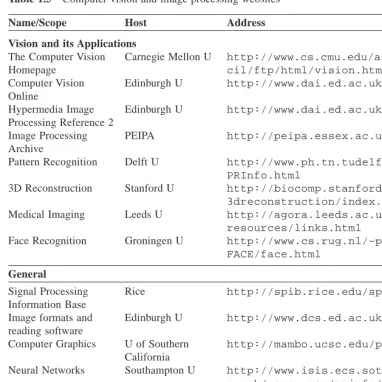
information flow during processing. However, the underlying mathematics is not made clear to the user, as it can be when a mathematical system is used. There is a new textbook, and a very readable one at that, by Nick Efford (Efford, 2000) which is based entirely on Java and includes, via a CD, the classes necessary for image processing software development. A set of WWW links are shown in Table 1.2 for established freeware and commercial software image processing systems. What is perhaps the best selection can be found at the general site, from the computer vision homepage software site (repeated later in Table 1.5).
Table 1.2 Software package websites
Packages (freeware or student version indicated by *)
General Site Carnegie Mellon http://www.cs.cmu.edu/afs/cs/ project/cil/ftp/html/v-source.html
Khoros Khoral Research http://www.khoral.com/
Hannover U http://www.tnt.uni-hannover.de/ soft/imgproc/khoros/
AdOculos* The Imaging Source http://www.theimagingsource.com/
(+ Textbook) catalog/soft/dbs/ao.htm
CVIPtools* Southern Illinois U http://www.ee.siue.edu/CVIPtools/
LaboImage* Geneva U http://cuiwww.unige.ch/~vision/
LaboImage/labo.html
TN-Image* Thomas J. Nelson http://las1.ninds.nih.gov/tnimage-manual/tnimage-manual.html
1.5 Mathematical systems
In recent years, a number of mathematical systems have been developed. These offer what is virtually a word-processing system for mathematicians and many are screen-based using a Windows system. The advantage of these systems is that you can transpose mathematics pretty well directly from textbooks, and see how it works. Code functionality is not obscured by the use of data structures, though this can make the code appear cumbersome. A major advantage is that the system provides the low-level functionality and data visualisation schemes, allowing the user to concentrate on techniques alone. Accordingly, these systems afford an excellent route to understand, and appreciate, mathematical systems prior to development of application code, and to check the final code functions correctly.
1.5.1 Mathematical tools
perhaps the two most popular of the mathematical systems. We shall describe Matlab later, as it is different from Mathcad, though the aim is the same. The website links for the main mathematical packages are given in Table 1.3.
Table 1.3 Mathematical package websites
General
Math-Net Links to the Math-Net http://www.math-net.de/ Mathematical World (Germany)
Vendors
Mathcad MathSoft http://www.mathcad.com/
Mathematica Wolfram Research http://www.wri.com/
Matlab Mathworks http://www.mathworks.com/
1.5.2 Hello Mathcad, Hello images!
The current state of evolution is Mathcad 2001; this adds much to version 6 which was where the system became useful as it included a programming language for the first time. Mathcad offers a compromise between many performance factors, and is available at low cost. If you do not want to buy it, there was a free worksheet viewer called Mathcad Explorer which operates in read-only mode. There is an image processing handbook available with Mathcad, but it does not include many of the more sophisticated feature extraction techniques.
Mathcad uses worksheets to implement mathematical analysis. The flow of calculation is very similar to using a piece of paper: calculation starts at the top of a document, and flows left-to-right and downward. Data is available to later calculation (and to calculation to the right), but is not available to prior calculation, much as is the case when calculation is written manually on paper. Mathcad uses the Maple mathematical library to extend its functionality. To ensure that equations can migrate easily from a textbook to application, Mathcad uses a WYSIWYG (What You See Is What You Get) notation (its equation editor is actually not dissimilar to the Microsoft Equation (Word) editor).
Images are actually spatial data, data which is indexed by two spatial co-ordinates. The camera senses the brightness at a point with co-ordinates x, y. Usually, x and y refer to the horizontal and vertical axes, respectively. Throughout this text we shall work in orthographic
projection, ignoring perspective, where real world ordinates map directly to x and y
40 30 20 10 0 2 4 6 6 pic : =
1 2 3 4 1 1 2 1
2 2 3 2 1 2 2 1
3 1 38 39 37 36 3 1 4 1 45 44 41 42 2 1 1 2 43 44 40 39 1 3 2 1 39 41 42 40 2 1
1 2 1 2 2 3 1 1
1 2 1 3 1 1 4 2
pic
(a) Matrix (b) Surface plot (c) Image
Consider, for example, the matrix of pixel values in Figure 1.13(a). This can be viewed as a surface (or function) in Figure 1.13(b), or as an image in Figure 1.13(c). In Figure 1.13(c) the brightness of each point is proportional to the value of its pixel. This gives the synthesised image of a bright square on a dark background. The square is bright where the pixels have a value around 40 brightness levels; the background is dark, these pixels have a value near 0 brightness levels. This image is first given a label, pic, and then pic is allocated, :=, to the matrix defined by using the matrix dialog box in Mathcad, specifying a matrix with 8 rows and 8 columns. The pixel values are then entered one by one until the matrix is complete (alternatively, the matrix can be specified by using a subroutine, but that comes later). Note that neither the background, nor the square, has a constant brightness. This is because noise has been added to the image. If we want to evaluate the performance of a computer vision technique on an image, but without the noise, we can simply remove it (one of the advantages to using synthetic images). The matrix becomes an image when it is viewed as a picture, as in Figure 1.13(c). This is done either by presenting it as a surface plot, rotated by zero degrees and viewed from above, or by using Mathcad’s picture facility. As a surface plot, Mathcad allows the user to select a greyscale image, and the patch plot option allows an image to be presented as point values.
Figure 1.13 Synthesised image of a square
Mathcad stores matrices in row-column format. The co-ordinate system used throughout this text has x as the horizontal axis and y as the vertical axis (as conventional). Accordingly,
x is the column count and y is the row count so a point (in Mathcad) at co-ordinates x,y
is actually accessed as picy,x. The origin is at co-ordinates x = 0 and y = 0 so pic0,0 is the magnitude of the point at the origin and pic2,2 is the point at the third row and third column and pic3,2 is the point at the third column and fourth row, as shown in Code 1.1 (the points can be seen in Figure 1.13(a)). Since the origin is at (0,0) the bottom right-hand point, at the last column and row, has co-ordinates (7,7). The number of rows and the number of columns in a matrix, the dimensions of an image, can be obtained by using the Mathcad rows and cols functions, respectively, and again in Code 1.1.
pic2,2=38 pic3,2=45
rows(pic)=8 cols(pic)=8
This synthetic image can be processed using the Mathcad programming language, which can be invoked by selecting the appropriate dialog box. This allows for conventional for, while and if statements, and the earlier assignment operator which is := in non-code sections is replaced by ← in sections of code. A subroutine that inverts the brightness level at each point, by subtracting it from the maximum brightness level in the original image, is illustrated in Code 1.2. This uses for loops to index the rows and the columns, and then calculates a new pixel value by subtracting the value at that point from the maximum obtained by Mathcad’s max function. When the whole image has been processed, the new picture is returned to be assigned to the label newpic. The resulting matrix is shown in Figure 1.14(a). When this is viewed as a surface, Figure 1.14(b), the inverted brightness levels mean that the square appears dark and its surroundings appear white, as in Figure 1.14(c).
New_pic:= for x∈0..cols(pic)–1
for y∈0..rows(pic)–1
newpicturey,x ←max(pic)–picy,x
newpicture
Code 1.2 Processing image points in Mathcad
Routines can be formulated as functions, so they can be invoked to process a chosen
picture, rather than restricted to a specific image. Mathcad functions are conventional, we simply add two arguments (one is the image to be processed, the other is the brightness to be added), and use the arguments as local variables, to give the add function illustrated in Code 1.3. To add a value, we simply call the function and supply an image and the chosen brightness level as the arguments.
Figure 1.14 Image of a square after inversion
add_value(inpic,value):= for x 0..cols(inpic)–1 for y 0..rows(inpic)–1
newpicturey,x ←inpicy,x+value
newpicture
Code 1.3 Function to add a value to an image in Mathcad 6 40 30 20 10 0 2 4 6
(a) Matrix (b) Surface plot (c) Image
new_pic =
44 43 42 41 44 44 43 44 43 43 42 43 44 43 43 44
42 44 7 6 8 9 42 44
41 44 0 1 4 3 43 44
44 43 2 1 5 6 44 42
43 44 6 4 3 5 43 44
44 43 44 43 43 42 44 44 44 43 44 42 44 44 41 43
Mathematically, for an image which is a matrix of N × N points, the brightness of the pixels in a new picture (matrix), N, is the result of adding b brightness values to the pixels in the old picture, O, given by:
Nx,y = Ox,y + b ∀x, y ∈ 1, N (1.1)
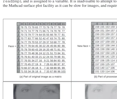
Real images naturally have many points. Unfortunately, the Mathcad matrix dialog box only allows matrices that are 10 rows and 10 columns at most, i.e. a 10 × 10 matrix. Real images can be 512 × 512, but are often 256 × 256 or 128 × 128, this implies a storage requirement for 262144, 65536 and 16384 pixels, respectively. Since Mathcad stores all points as high precision, complex floating point numbers, 512 × 512 images require too much storage, but 256 × 256 and 128 × 128 images can be handled with ease. Since this cannot be achieved by the dialog box, Mathcad has to be ‘tricked’ into accepting an image of this size. Figure 1.15 shows the image of a human face captured by a camera. This image has been stored in Windows bitmap (.BMP) format. This can be read into a Mathcad worksheet using the READBMP command (yes, capitals please! – Mathcad can’t handle
readbmp), and is assigned to a variable. It is inadvisable to attempt to display this using the Mathcad surface plot facility as it can be slow for images, and require a lot of memory.
[image:30.595.55.438.281.607.2](c) Bitmap of original image
Figure 1.15 Processing an image of a face
0 1 2 3 4 5 6 7 8 9 10 11 12
0 1 2 3 4 5 6 7 8
158 155 153 159 163 157 153 159 159 154 151 154 157 159 151 146 151 154 150 153 159 157 154 144 135 135 146 150 157 163 157 146 132 122 127 143 154 157 159 150 133 117 109 117 133 156 157 158 144 125 110 102 106 125 155 159 158 140 123 108 96 100 128 156 157 150 128 116 104 92 101 131 155 156 141 120 113 101 92 104 135 157 156 135 114 107 96 89 101 136 157 150 125 107 90 89 87 106 141 153 140 117 106 98 85 87 112 148 151 133 114 106 98 86 87 113 147 New face =
0 1 2 3 4 5 6 7 8 9 10 11 12
0 1 2 3 4 5 6 7 8 9 10 11 78 75 73 79 83 77 73 79 79 77 79 78 74 71 74 77 79 71 66 71 74 79 79 77 70 73 79 77 74 64 55 55 66 78 77 81 70 77 83 77 66 52 42 47 63 74 75 80 74 77 79 70 53 37 29 37 53 68 77 78 76 77 78 64 45 30 22 26 45 66 80 86 75 79 78 60 43 28 16 20 48 71 81 91 76 77 70 48 36 24 12 21 51 73 84 91 75 76 61 40 33 21 12 24 55 79 88 91 77 76 55 34 27 16 9 21 56 84 93 95 77 70 45 27 19 9 7 26 61 88 97 97 73 60 37 26 18 5 7 32 68 88 95 99 71 53 34 26 18 6 7 33 67 88 96 103 Face =
(a) Part of original image as a matrix (b) Part of processed image as a matrix
It is best to view an image using Mathcad’s picture facility or to store it using the WRITEBMP
command, and then look at it using a bitmap viewer.
So if we are to make the image of the face brighter, by addition, by the routine in Code 1.3, via the code in Code 1.4, the result is as shown in Figure 1.15. The matrix listings in Figure 1.15(a) and Figure 1.15(b) show that 80 has been added to each point (these only show the top left-hand section of the image where the bright points relate to the blonde hair, the dark points are the gap between the hair and the face). The effect will be to make each point appear brighter as seen by comparison of the (darker) original image, Figure 1.15(c), with the (brighter) result of addition, Figure 1.15(d). In Chapter 3 we will investigate techniques which can be used to manipulate the image brightness to show the face in a much better way. For the moment though, we are just seeing how Mathcad can be used, in a simple way, to process pictures.
The translation of the Mathcad code into application can be rather prolix when compared with the Mathcad version by the necessity to include low-level functions. Since these can obscure the basic image processing functionality, Mathcad is used throughout this book to show you how the techniques work. The translation to application code is perhaps easier via Matlab (it offers direct compilation of the code). There is also an electronic version of this book which is a collection of worksheets to help you learn the subject; and an example Mathcad worksheet is given in Appendix 3 (Section 9.3). You can download these worksheets from this book’s website (http://www.ecs.soton.ac.uk/~msn/book/) and there is a link to Mathcad Explorer there too. You can then use the algorithms as a basis for developing your own application code. This provides a good way to verify that your code
mach := face
mach := for x∈0..cols(mach)–1
for y∈0..rows(mach)–1
machy,x←40·floor
x 21.5
mach
Code 1.5 Creating the Image of Figure 1.4(a)
face :=READBMP(rhdark) newface :=add_value(face,80) WRITEBMP(rhligh) :=newface
Code 1.4 Processing an image
actually works: you can compare the results of your final application code with those of the original mathematical description. If your final application code and the Mathcad implementation are both correct, the results should be the same. Naturally, your application code will be much faster than in Mathcad, and will benefit from the GUI you’ve developed.
1.5.3 Hello Matlab!
Matlab is rather different from Mathcad. It is not a WYSIWYG system but instead it is more screen-based. It was originally developed for matrix functions, hence the ‘Mat’ in the name. Like Mathcad, it offers a set of mathematical tools and visualisation capabilities in a manner arranged to be very similar to conventional computer programs. In some users’ views, a WYSIWYG system like Mathcad is easier to start with but there are a number of advantages to Matlab, not least the potential speed advantage in computation and the facility for debugging, together with a considerable amount of established support. Again, there is an image processing toolkit supporting Matlab, but it is rather limited compared with the range of techniques exposed in this text. The current version is Matlab 5.3.1, but these systems evolve fast!
Essentially, Matlab is the set of instructions that process the data stored in a workspace, which can be extended by user-written commands. The workspace stores the different lists of data and these data can be stored in a MAT file; the user-written commands are functions that are stored in M-files (files with extension .M). The procedure operates by instructions at the command line to process the workspace data using either one of Matlab’s own commands, or using your own commands. The results can be visualised as graphs, surfaces or as images, as in Mathcad.
The system runs on Unix/Linux or Windows and on Macintosh systems. A student version is available at low cost. There is no viewer available for Matlab, you have to have access to a system for which it is installed. As the system is not based around worksheets, we shall use a script which is the simplest type of M-file, as illustrated in Code 1.6. To start the Matlab system, type MATLAB at the command line. At the Matlab prompt (>>) type
chapter1 to load and run the script (given that the file chapter1.m is saved in the directory you are working in). Here, we can see that there are no text boxes and so comments are preceded by a %. The first command is one that allocates data to our variable
pic. There is a more sophisticated way to input this in the Matlab system, but that is not available here. The points are addressed in row-column format and the origin is at co-ordinates y = 1 and x = 1. So we then access these point pic3,3 as the third column of the third row and pic4,3 is the point in the third column of the fourth row. Having set the display facility to black and white, we can view the array pic as a surface. When the surface, illustrated in Figure 1.16(a), is plotted, then Matlab has been made to pause until you press Return before moving on. Here, when you press Return, you will next see the image of the array, Figure 1.16(b).
%Chapter 1 Introduction (Hello Matlab) CHAPTER1.M %Written by: Mark S. Nixon
disp(‘Welcome to the Chapter1 script’)
disp(‘This worksheet is the companion to Chapter 1 and is an introduction.’)
disp(‘It is the source of Section 1.4.3 Hello Matlab.’)
disp(‘The worksheet follows the text directly and allows you to process basic images.’)
disp(‘Let us define a matrix, a synthetic computer image called pic.’)
pic = [1 2 3 4 1 1 2 1;
2 2 3 2 1 2 2 1;
3 1 38 39 37 36 3 1;
4 1 45 44 41 42 2 1;
1 2 43 44 40 39 1 3;
2 1 39 41 42 40 2 1;
1 2 1 2 2 3 1 1;
1 2 1 3 1 1 4 2]
%Pixels are addressed in row-column format.
%Using x for the horizontal axis(a column count), and y for the vertical axis (a row
%count) then picture points are addressed as pic(y,x). The origin is at co-ordinates
%(1,1), so the point pic(3,3) is on the third row and third column; the point pic(4,3)
%is on the fourth row, at the third column. Let’s print them: disp (‘The element pic(3,3)is’)
pic(3,3)
disp(‘The element pic(4,3)is’) pic(4,3)
%We’ll set the output display to black and white colormap(gray);
%We can view the matrix as a surface plot
disp (‘We shall now view it as a surface plot (play with the controls to see it in relief)’)
disp(‘When you are ready to move on, press RETURN’) surface(pic);
%Let’s hold a while so we can view it pause;
%Or view it as an image
disp (‘We shall now view the array as an image’) disp(‘When you are ready to move on, press RETURN) imagesc(pic);
%Let’s hold a while so we can view it pause;
disp(‘The dimensions of the array are’) size(pic)
%now let’s invoke a routine that inverts the image inverted_pic=invert(pic);
%Let’s print it out to check it
disp(‘When we invert it by subtracting each point from the maximum, we get’)
inverted_pic %And view it
disp(‘And when viewed as an image, we see’)
disp(‘When you are ready to move on, press RETURN’) imagesc(inverted_pic);
%Let’s hold a while so we can view it pause;
disp(‘We shall now read in a bitmap image, and view it’) disp(‘When you are ready to move on, press RETURN’) face=imread(‘rhdark.bmp’,‘bmp’);
imagesc(face); pause;
%Change from unsigned integer(unit8) to double precision so we can process it
face=double(face);
disp(‘Now we shall invert it, and view the inverted image’) inverted_face=invert(face);
imagesc(inverted_face);
disp(‘So we now know how to process images in Matlab. We shall be using this later!’)
Code 1.6 Matlab script for chapter 1
(a) Matlab surface plot
Figure 1.16 Matlab image visualisation 50
40
30
20
10
0 8
6
4 2
0 1 2 3 4
5 6 7
8
(b) Matlab image 1
2
3
4
5
6
7
8