White Rose Research Online URL for this paper:
http://eprints.whiterose.ac.uk/113087/
Article:
Gyenge, N., Singh, T., Kiss, T.S. et al. (2 more authors) Active longitude and CME
occurrences. (Unpublished)
[email protected] https://eprints.whiterose.ac.uk/
Reuse
Unless indicated otherwise, fulltext items are protected by copyright with all rights reserved. The copyright exception in section 29 of the Copyright, Designs and Patents Act 1988 allows the making of a single copy solely for the purpose of non-commercial research or private study within the limits of fair dealing. The publisher or other rights-holder may allow further reproduction and re-use of this version - refer to the White Rose Research Online record for this item. Where records identify the publisher as the copyright holder, users can verify any specific terms of use on the publisher’s website.
Takedown
If you consider content in White Rose Research Online to be in breach of UK law, please notify us by
Draft version February 23, 2017
Preprint typeset using LATEX style emulateapj v. 12/16/11
ACTIVE LONGITUDES AND OCCURRENCE OF CORONAL MASS EJECTIONS
N. Gyenge1,2*, T. Singh3, T. S. Kiss1,4, A. K. Srivastava3, R. Erd´elyi1
1
Solar Physics and Space Plasmas Research Centre (SP2RC), School of Mathematics and Statistics, University of Sheffield Hounsfield Road, Hicks Building, Sheffield S3 7RH, UK
2
Debrecen Heliophysical Observatory (DHO), Konkoly Observatory, Research Centre for Astronomy and Earth Sciences Hungarian Academy of Sciences, Debrecen, P.O.Box 30, H-4010, Hungary
3
Department of Physics, Indian Institute of Technology (Banaras Hindu University), Varanasi, India 4
Department of Physics, University of Debrecen, Egyetem t´er 1, Debrecen, H-4010, Hungary
Draft version February 23, 2017
ABSTRACT
The spatial inhomogeneity of the distribution of coronal mass ejection (CME) occurrences in the solar atmosphere could provide a tool to estimate the longitudinal position of the most probable CME-capable active regions in the Sun. The anomaly in the longitudinal distribution of active regions themselves is often referred to as active longitude (AL). In order to reveal the connection between the AL and CME spatial occurrences, here we investigate the morphological properties of active regions. The first morphological property studied is the separateness parameter, which is able to characterise the probability of the occurrence of an energetic event, such as solar flare or CME. The second morphological property is the sunspot tilt angle. The tilt angle of sunspot groups allows us to estimate the helicity of active regions. The increased helicity leads to a more complex built-up of the magnetic structure and also can cause CME eruption. We found that the most complex active regions appear near to the AL and the AL itself is associated with the most tilted active regions. Therefore, the number of CME occurrences is higher within the AL. The origin of the fast CMEs is also found to be associated with this region. We concluded that the source of the most probably CME-capable active regions is at the AL. By applying this method we can potentially forecast a flare and/or CME source several Carrington rotations in advance. This finding also provides new information for solar dynamo modelling.
1. SOLAR NON-AXISYMMETRIC ACTIVITY
Since the beginning of the last century the non-homogeneous spatial properties of solar activity have been studied extensively (Carrington 1863;Chidambara
1932;Maunder 1905;Losh 1939;Bumba 1965;Bumba &
Obridko 1969). These early investigations conjectured
initially that the longitudinal distribution of sunspot groups or sunspot numbers shows non-homogeneous be-haviour. These analyses concluded that there are pre-ferred longitudes, where solar activity concentrates.
Later, different approximations and assumptions were applied to understand the essence of this phenomenon. The topic soon became controversial (see e.g.Pelt et al.
2006;Henney & Durney 2005). Overall, three approaches
can be distinguished. The first approach is the quasi-rigid structure model byWarwick(1966). This model de-scribes a constantly rotating frame which carries the per-sistent domains of activity (Ivanov 2007). Bogart(1982) applied an autocorrelation statistical method based on long-term sunspot number data. Balthasar & Sch¨ussler
(1983, 1984) applied period-analysis to the Greenwich Photoheliographics Results (GPR). These studies con-cluded that the angular velocity of the quasi-rigid rotat-ing frame varies. The angular velocity depends on the solar cycle, but during one cycle the angular velocity is constant.
The second approach, promoted by e.g.Becker(1955);
Castenmiller et al. (1986) andBrouwer & Zwaan(1990)
*
e-mail: [email protected]
discovered the ’active nest’ and defined it as a small and isolated area on the solar surface. Here, the enhanced longitudinal activities are considered as individual enti-ties. These isolated entities can be absent for several rotations.
The third group of models assumes a migrating activ-ity in the Carrington coordinate system. Berdyugina &
Usoskin (2003); Berdyugina (2004, 2005) found
persis-tent ALs under the influence of the differential rotation.
Usoskin et al.(2005) andBerdyugina et al.(2006)
intro-duced a ’dynamic reference frame’. This frame describes the longitudinal migration of active longitude in Car-rington coordinate system and the frame has a similar dynamics to differential rotation. Usoskin et al. (2007) concluded that the migration of the enhanced activity is just apparent. In the ’dynamic reference frame’, the ro-tation of the active longitude remains constant and the active longitude itself is a persistent quasi-rigidly rotat-ing phenomenon. Usoskin et al. (2007) proposed that a seemingly migrating AL may occur as a result of in-teraction between the equatorward propagating dynamo wave and a quasi-rigidly rotating non-axisymmetric ac-tive zone. The role of differential rotation is also con-troversy. Various studies concluded that the differential rotation is not the reason of the migration of the AL
(Balthasar 2007;Juckett 2006,2007;Gyenge et al. 2014).
In our previous work (i.e. Gyenge et al. (2016), here-after GY16), we found evidence supporting the third group of models. Moreover, the migration of ALs does not appear to correspond very well to the form of the 11-year cycle as suggested by previous studies (Usoskin
et al. 2005; Berdyugina et al. 2006). The half-width of the active longitudinal belt is fairly narrow during mod-erate activity but is wider at maximum activity. We also found that the AL is not always identifiable.
Several studies (Warwick 1965;Bai 2003a,b) suggested that the spatial distributions of eruptive solar phenom-ena also show non-axisymmetric properties. Bai (1987,
1988) analysed the coordinates of energetic solar flares based of 5 years of time period and concluded that longi-tudinal spatial distribution is non-homogeneous. Zhang
et al. (2007, 2008, 2015) concluded that the dominant
and co-dominant AL contains 80% of C- and X-flares. In GY16, we conducted a similar study based on four solar cycles and we did not find significant co-dominant activity; instead, we found that only the dominant AL contains 60% of the solar flares.
The flares and CMEs could occur independently of each other. Numerous CMEs have associated flares but several non-flaring filament lift-offs also lead to CME
(Gosling et al. 1976; Harrison 1995). Furthermore, in
the case of the ’stealth’ CMEs there are no easily identi-fiable signatures to locate the source of the eruption on the solar surface (Howard 2013). Hence, separate flare -CME spatial distribution investigations are justified.
2. CME AND SUNSPOT DATA
We used the SOHO/LASCO HALO CME catalog by
the CDAW data centre1. The CME catalog spans over
20 years, i.e. between 1996 and 2016. This is the most extensive catalog that contains the source location of CMEs. Only halo CMEs are reported, i.e. their angular width is 360 degrees in C3 coronagraph Field of View.
Gopalswamyet al.(2009) describes the catalog in great
details. The CME source is defined as the centre of the associated active region. The source of the CME is iden-tified using SOHO EIT running difference images. Later, the ability of the STEREO mission to observe the back-side of Sun was used to identify the source of back-back-sided halo CMEs (Gopalswamyet al.2015). This catalog also provides the space speed of CMEs which is the actual speed with which the CME propagates in the interplan-etary space. The Plane of Sky speed obtained from the single SOHO viewpoint, converted into space speed using the cone model (Xieet al.2004).
The Debrecen Photoheliographic Data2 (DPD)
sunspot catalogue is used for estimating the longitudinal position of the AL. The catalog provides information about the date of observation, position and area for each sunspot. The precision of the position is 0.1 heliographic degrees and the estimated accuracy of the area measurement is ∼10 percent.
3. LONGITUDINAL SUNSPOT DISTRIBUTION
The first step of our identification procedure is to di-vide the solar surface by 18 equally sliced longitudinal belts. Hence, one bin equals to a zone with 20◦ width. We take into account all sunspot groups from the mo-ment when they reach their maximum area. This filtering criteria is chosen for the following reasons: Firstly, if we select all sunspot groups at every moment of time then
1http://cdaw.gsfc.nasa.gov/CME_list/halo/halo.html 2
http://fenyi.solarobs.unideb.hu/DPD/
the statistics will be biased by the long-lived sunspot groups. Secondly, the maximum area of the sunspot groups is a well-defined and easily identifiable moment. This is different from the used practice of considering only the first appearance of each sunspot group. Let us define the matrixW by:
Wλ,CR=
Ai,CR Pn
i=1Ai,CR
. (1)
Here, the area of all sunspot groups (Ai,CR) is summed
up in each longitudinal bin for each CR. Ai,CR is
di-vided by the summarised area over the entire solar sur-face (Pn
i=1Ai,CR). The range ofW must be always
be-tween 0 and 1, depending on the local appearance of the activity. In the case of Wλ,CR= 1, all of the flux
emer-gence takes place in one single longitudinal strip. A 3σ significance level threshold is applied to filter the noise. Moving average is also applied for data smoothing with a time-window of 3 CRs.
We standardised the matrixWλ,CR(defined in Eq1) by
removing the mean of the data and scaling to unit vari-ance. Then, cluster analysis was performed for group-ing the obtained significant peaks. Here, the DBSCAN clustering algorithm was chosen which is a density-based algorithm. The method groups together points that are relatively closely packed together in a high-density re-gion and it marks outlier points that stand alone in low-density regions (for details seeEster et al.(1996)). The parameter epsilon (= 0.2) defines the maximum distance between two points to be considered to be in the same group. The parameter m (= 3) specifies the desired min-imum cluster size. Clusters, containing less than three points, were omitted. The longitudinal location of the clusters (λcluster,CR) represent the position of the AL.
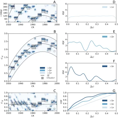
Panel A of Figure 1 shows an example of the initial identification steps outlined above. The sample time pe-riod covers 6 years, and it corresponds to 80 CR between 1920 CR and 2000 CR. The quantity W is represented by the shades with blue colour. The dark blue regions denote the significance (3σ) presence of activity. The brighter shades stand for a weaker manifestation of ac-tivity (2σand 1σ). The grey squares shows the sunspot group clusters.
In PanelBof Figure1, the Carrington longitudes of the most significant cluster is transformed into Carrington Phase for each CR:
ψAl, CR=
λcluster, CR
360 . (2)
The range of the quantityψALmust be between 0 and 1
whereψAL = 1 represents the entire circumference of the
Sun. In PanelB of Figure1, PanelA is repeated three times so that we are able to track the migration of the activity thought the phases. To the data Panels A and B, we applied a polynomial least squares fitting based on multiple models. Linear, quadratic, cubic and higher-order polynomial models were tested. The quadratic or parabolic regression (Ax2+Bx−C) shows the best
good-ness of fit, hence this model is chosen. Table1shows the coefficients and uncertainties.
The shape of migration clearly follows parabolic-shaped path as found in several earlier studies (
Active longitude and CME occurrences 3
1920 1940 1960 1980 2000 CR
0 60 120 180 240 300 360
λ
[d
eg
]
A
1920 1940 1960 1980 2000 CR
0.0 0.5 1.0 1.5 2.0 2.5 3.0
ψAl
B
>3σ >2σ >1σ Al Cluster
1920 1940 1960 1980 2000 CR
0.0 0.2 0.4 0.6 0.8 1.0
ψAl
C
0.0 0.1 0.2 0.3 0.4 0.5
∆ψ
0 2 4 6
D
>1σ
0.0 0.1 0.2 0.3 0.4 0.5
∆ψ
0 2 4 6
E
>2σ
0.0 0.1 0.2 0.3 0.4 0.5
∆ψ
0 2 4 6 8
F
>3σ
0.0 0.1 0.2 0.3 0.4 0.5
∆ψ
0.0 0.2 0.4 0.6 0.8 1.0
CDF
G
[image:4.612.105.513.63.468.2]>3σ >2σ >1σ
Fig. 1.—The PanelsA,BandCshow an example of the migration of the active longitude between 1920 CR and 2000 CR (01/03/1997-20/02/2003) based on data of the solar northern hemisphere. The shades of blue indicates the significance of sunspot group activity. The grey squares show high-density areas, i.e. the detected clusters. The solid black line represents the migration patch, fitted by the least-square-method and considering only the most significant (above 3σ) clusters. PanelAshows the observed longitudinal distribution of sunspots in Carrington coordinate system. PanelB, similar to PanelA, depicts solar circumference (Carrington phase) repeated three times. PanelCis the phase-corrected migration path. The parabolic migration pattern is now transformed to a constant line, and provides an insight into the non-homogeneous spatial property. The panelsAandC use the same colour scale as defined in Panel B. The colour scale is displayed in the lower right corner of the PanelB. PanelsD,EandF show the sunspot distribution around the active longitude (corresponding to ∆ψ= 0) with different significance levels taken for the entire time period and for both hemispheres. The horizontal axes (∆ψ- Carrington Phase Difference) represent the shortest distance between the migration of enhanced longitudinal activity and given sunspot groups. PanelGis the cumulative distribution of the above three PDF.
2011a; Usoskin et al. 2007, 2005; Gyenge et al. 2014).
In Panel C of Figure1, let us now plot the parabola-shaped migration path in a coordinate system that fol-lows the parabolic shape of Panel B. Hence, the active longitude is easily recognisable without repeating Car-rington Phases. Several new features are noticeable in Panel C; parallel aligned and tilted lanes between CR 1930 and CR 1950. These shapes are artificial, created by the coordinate system transformation. In the new dynamic coordinate system the AL stands still as repre-sented by the black regression line.
PanelsD, E andF of Figure1show the kernel density estimation (KDE) of the spatial difference between the AL (ψAL,CR) and the longitudinal position of
individ-ual sunspot groups (ψCR) in Carrington phase difference
(∆ψ, see Eq. 3) applied to the entire period investigated (i.e between 06/01/1997 and 30/12/2015) and for both hemispheres.
∆ψ∗=|ψ
Al, CR−ψCR|,
∆ψ=
∆ψ∗, if ∆ψ∗≤0.5, 1−∆ψ∗, if ∆ψ∗>0.5.
(3)
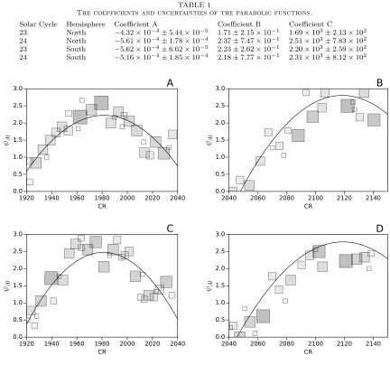
loca-TABLE 1
The coefficients and uncertainties of the parabolic functions.
Solar Cycle Hemisphere Coefficient A Coefficient B Coefficient C 23 North −4.32×10⁻⁴±5.44×10⁻⁵ 1.71±2.15×10⁻¹ 1.69×10³±
2.13×10² 24 North −5.61×10⁻⁴±1.78×10⁻⁴ 2.37±7.47×10⁻¹ 2.51×10³±7.83×10² 23 South −5.62×10⁻⁴±6.62×10⁻⁵ 2.23±2.62×10⁻¹ 2.20×10³±2.59×10² 24 South −5.16×10⁻⁴±1.85×10⁻⁴ 2.18±7.77×10⁻¹ 2.31×10³±8.12×10²
1920 1940 1960 1980 2000 2020 2040 CR
0.0 0.5 1.0 1.5 2.0 2.5 3.0
ψAl
A
2040 2060 2080 2100 2120 2140 CR
0.0 0.5 1.0 1.5 2.0 2.5 3.0
ψAl
B
1920 1940 1960 1980 2000 2020 2040 CR
0.0 0.5 1.0 1.5 2.0 2.5 3.0
ψAl
C
2040 2060 2080 2100 2120 2140 CR
0.0 0.5 1.0 1.5 2.0 2.5 3.0
ψAl
D
Fig. 2.—The four panels demonstrate the phase-corrected migration path based on the entire analysed period. The PanelsAandC
show the AL in Solar Cycle 23 and the PanelsBandD in Solar Cycle 24. PanelsAandBdemonstrate the northern hemisphere data and PanelsCandDshow the southern hemisphere. The grey squares visualise the result of the DBSCAN algorithm, i.e. the detected and significant sunspot group clusters. The quadratic model function is applied. The coefficients and uncertainties are given in Table1.
tion of the sunspot groups are shifted by 180 degrees from the position of the AL. This shifted position is marking the area of the co-dominant AL. The three KDEs are ob-tained from different sunspot group datasets with differ-ent threshold levels. PanelF of Figure1shows the most significant regions (3σsignificance threshold was applied) which tend to be formed near the active longitude. The less significant (2σ) sunspot groups show a more disperse distribution. Below the 1σthreshold, the KDE does not show obvious peaks. PanelGof Figure 1depicts cumu-lative distribution functions (CDF) of the three KDEs. Note that 70% of the most significant sunspot groups ap-pear closer than ∆ψ= 0.17. This value corresponds to a longitudinal zone with±60 degrees of width around AL. The Figure 2 show the migration path of the AL based on the entire analysed period. The coefficients and un-certainties of the employed quadratic model functions are displayed in Table1.
4. COMPLEXITY PROPERTIES OF AL SUNSPOTS
4.1. Separateness parameter
The relationship between flare occurrences and the morphological properties of sunspot groups is widely ac-cepted and is reported in numerous studies (e.g.
Schri-jver et al. 2007;Cui et al. 2006;Mason & Hoeksema 2010;
Kors´os et al. 2014,2015b). The first classification scheme
(Haleet al.1919) is published byWaldmeier(1938). The scheme examines the role of the size and morphology of sunspot groups in relation of determining the capacity of their flare-productivity. The system was modified by
Waldmeier (1947) and is known today as the modified
[image:5.612.91.523.68.472.2]Active longitude and CME occurrences 5
294 296 298 300 302 304 L [deg]
12 14 16 18 20 22
B [deg]
S=0.6±0.25
400 350 300 250
Y [arcsec] 320
340 360 380 400 420 440 460
X [arcsec]
AR11429 2012-03-07 15:02:44
84 86 88 90 92 94 96 98 L [deg]
4 6 8 10 12 14
B [deg]
S=1.3±0.35
200 250 300 350 400 Y [arcsec]
200 250 300 350
X [arcsec]
AR11666 2011-03-10 15:02:45
107 108 109 110 111 112 113 114 L [deg]
17 18 19 20 21 22
B [deg]
S=2.0±0.3
160 180 200 220 240 Y [arcsec]
240 260 280 300 320
X [arcsec]
[image:6.612.107.508.64.503.2]AR11241 2011-06-25 15:02:56
Fig. 3.—Representation of the reconstructed sunspot groups (left-hand side) using the Debrecen Sunspot Data (DPD) catalogue applied to active regions NOAA 11429 (07/03/2012 15:02:44), NOAA 11666 (0/03/2011 15:02:45), NOAA 11241 (25/06/2011 15:02:26). The polarities of the spots are distinguished by the different colours (red and blue). The grey colour is the hypothetical circle, having summarized area of the group. The dashed line is the distance between the following and leading subgroups. The area is measured in MSH (millionths of solar hemisphere). The sunspots are corrected for foreshortening. On the right-hand side, the magnetograms of the example sunspot groups are displayed.
number of classes (Bornmann & Shaw 1994).
The separateness parameter (S) is used to reveal the morphological properties of the sunspot groups near and far from the AL. This parameter was introduced by
Kors´os et al. (2015b) and its investigation and
applica-tion to flares showed that the separateness parameter can be a numerical indicator/precursor besides the tra-ditional (Z¨urich, McIntosh and Mount Wilson) classifica-tions of sunspot groups. The parameter S is considered as an indicator for the potential flaring outbreak and CME capability of active regions.
The separateness parameter is determined by the an-gular distance between the area-weighted centres of the leading and following subgroups divided by the
angu-lar diameter of a hypothetical circle whose area is equal to the total area of all umbrae constituting the sunspot group.
The angular distance is the shortest distance between two points on the surface of a sphere. The distance (in degrees) between the leading and following subgroups is provided by the spherical law of cosines:
∆θ= 2 arcsin
sin2(|Bl−Bf|
2 )+
+ cos(Bl) cos(Bf) sin2(
|Ll−Lf|
2 )
12
Here,B andLrefer to the heliographical latitude and longitude of l leading andf following subgroups. If the absolute difference is greater than 180 (|Ll−Lf|>180),
then the absolute difference is 360− |Ll−Lf|.
The corrected area of individual sunspots (A∗) in mil-lions of solar hemisphere is converted toM m2, using:
A= 1 2(4πR
2
Sun)10−7A∗, (5)
where RSun is in M m. The total sunspot group area
(T) is calculated. The number of sunspots in a certain sunspot group is represented by the quantityn. The total area (M m2) means the summed up area of the individual
sunspots:
T =
n
X
i=1
Ai. (6)
The diameter of an individual sunspot group, (∆Ω), is estimated by:
∆Ω = 2
p
T /π
2(RSuncos(12(Bl+Bf))π
360o. (7)
The numerator is the diameter (M m) of a hypothet-ical circle whose area is equal to theT total area. The denominator represents the circumference of small circle (M m), which connects all locations with a given latitude. The fraction is multiplied by 360 degrees, equals to the angular distance between the endpoints of the sunspot group diameter in degrees.
Finally, let us define the dimensionless separateness parameter:
S= ∆θ
∆Ω. (8)
In Figure3, typical active regions NOAA 11429, 11666 and 11241 (from top to bottom) are selected to demon-strate the usefulness of the parameter S. The visuali-sation of the active regions is plotted on the left-hand side. The blue and red colours distinguish the different magnetic polarities, the radius of a circle represents the area of the spot. The black dots indicate the weighted average position of the leading and following subgroups. The black dashed line between the black dots is the cal-culated angular distance (∆θ), described by the Eq. 4. The grey circle around the spots is the hypothetical cir-cle whose area is equal to the total area of all umbrae constituting the sunspot group (∆Ω), defined by Eq. 7. Panels on the right-hand side are the snapshots (HMI magnetogramm by SDO) of the active regions.
The upper two panels of the Figure 3 are visualising a complex sunspot group (namely, NOAA 11429). This sunspot group is a beta-gamma-delta magnetic configu-ration according to the Mount Wilson classification. The AR is extremely complex, having umbrae of opposite po-larity within the same penumbra. The calculated sepa-rateness parameter is 0.6±0.25 (Eq. 8). The middle pan-els of Figure3show NOAA Active Region 11666, which is a moderate complex sunspot group (S = 1.3±0.35). The bottom panels display NOAA Active Region 11241, a less complex bipolar sunspot group (S = 2.0±0.30)
Based on the study byKors´os et al.(2015b), there is a hight risk of X-class flare and/or fast CME occurrence(s) if S < 1. There is a moderate risk of flaring (M-class) and/or CME occurrence(s) if S >1 and S <2. In case of S >3, only bipolar sunspot groups appear with rela-tively simple morphological properties. These ARs have a rather low probability of a significant flaring (above GOES C-class) or CME activities.
4.2. Separateness parameter within AL
In this section, we investigate the longitudinal spatial distribution of the parameterS (Eq. 8) and the area of the investigated sunspot groups. The spatial distance of sunspot groups (∆ψ) is defined by Eq. 3.
The raw area measures are converted to standard scores (standardized statistics). The standard score is a dimensionless quantity calculated by subtracting the average of sunspot group area (T) from a given group area Ti and dividing by the sample-corrected standard
deviation (σ(T)) of the area data:
Zi=
Ti−T
σ(T) . (9)
Spatial multi-variable (linear) interpolation is applied to f(S,∆ψ, Z). The method results in a regular matrix (M) form unstructured 3-dimensional data. The range of logS is [−1,0.5], and is divided by 1500 equal bins (n). The range of ∆ψ[0,0.5] is divided by 500 bins (m), i.e.
M =
Z1,1 Z1,2 ... , Z1,n
Z2,1 Z2,2 ... , Z2,n
... ... ... , ... Zm,1 Zm,2 ... , Zm,n
. (10)
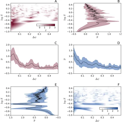
Figure 4 shows the results of the statistics. The pan-els A, B and C are obtained for data of the northern hemisphere (red-coloured plots) and panelsD,E andF are that of the southern hemisphere (blue-coloured fig-ures). In panelsA(northern hemisphere) andF (south-ern hemisphere), the matrix M (Eq. 10) is visualised. The horizontal axis is the distance from AL. The vertical axis is the logarithm of parameterS; logS <0 stands for a high-risk flare or CME occurrence. The colour code is the standard score of sunspot group area. The red or blue shades indicate positive standard score (Ti > T). The
white color stands for negative standard score (Ti < T
or no data). Panels B and E are the row averages of matrixM. Panels C andD are the column averages of matrixM.
In Panel A, significant islands are visible between 0>logS >−0.5 at ∆ψ <0.1. There is one more obvi-ously visible island around ∆ψ = 0.2 at logS < −0.4. However, above ∆ψ > 0.2 there is no remarkable is-land. Panel C of Figure 4 also reveals a peak below ∆ψ <0.1. The statistics suggests, that the most com-plex and largest sunspot groups appear near the AL.
Active longitude and CME occurrences 7
0.1 0.2 0.3 0.4
∆ψ
1.0 0.8 0.6 0.4 0.2 0.0 0.2 0.4
lo
g
S
A
0 1 2 3 Z
0.5 0.0 0.5 1.0 1.5
σ
1.0 0.8 0.6 0.4 0.2 0.0 0.2 0.4
lo
g
S
B
0.1 0.2 0.3 0.4
∆ψ
0.5 0.0 0.5 1.0 1.5 2.0
σ
C
0.1 0.2 0.3 0.4
∆ψ
1.0 0.8 0.6 0.4 0.2 0.0 0.2 0.4
lo
g
S
F
0 1 2 3 Z 0.5
0.0 0.5
1.0 1.5
σ
1.0 0.8 0.6 0.4 0.2 0.0 0.2 0.4
lo
g
S
E
0.1 0.2 0.3 0.4
∆ψ
0.5 0.0 0.5 1.0 1.5 2.0
σ
[image:8.612.101.509.70.477.2]D
Fig. 4.—The separateness - phase - standard score statistic based on the northern and souther hemisphere, indicated by blue and red colours. The panelsAandEshows the separateness of sunspot groups versus the longitudinal location of the active region. The shade of red and blue colours indicate the positive standard score. The PanelsB,C,DandE are the cross-section PDF, produced by the KDE method.
Both statistics suggest that the most complex active regions tend to cluster near the AL The co-dominant AL around ∆ψ = 0.5 does not have a significant activ-ity. This statistical investigation also highlights a non-equivalent AL and co-dominant AL activity.
4.3. Tilt angle of investigated Active Regions within AL
The last investigated morphological property of ARs, here, is the sunspot group tilt angle. The definition of the tilt angleγ∗ is given byHoward(1991);
γ∗= atan
(B
f−Bl)/(Lf−Ll)
sign(|Bf| − |Bl|) cos(B)
. (11)
ParametersB and L are the Carrington latitude and longitude. The following and leading subgroups have subscriptsf andl, respectively.
Figure5demonstrates the relationship found between
the separateness parameter S and scaled tilt angle γ = |γ∗/90|. Only most significant ARs are taken into ac-count; the area of sunspot groups has to be at least 2σ greater than average. The results applicable to the two hemispheres are distinguished by the colours of dots.
Linear regression cannot be used because the data is associated with a considerable uncertainty both in the X and Y directions (Isobe et al. 1990). For that rea-son, Principal Component Analysis (PCA) is used to fit the dataset. The PCA method is a linear dimensional-ity reduction keeping only the most significant singular vectors to project the data to a lower dimensional space
(Einbecket al. 2007). The eigenvector of the first
com-ponente1= [−0.8387,0.5445] shows the direction of the maximum variance of the data (σ2 = 4.1227), i.e where
the data is most spread out.
repre-0.8 0.6 0.4 0.2 0.0 0.2 0.4
log S
0.0 0.2 0.4 0.6 0.8 1.0
[image:9.612.76.271.60.267.2]γ
Fig. 5.—The tilt angle versus separateness parameter of sunspot groups for each hemispheres. Data from northern and souther hemispheres, respectively, are distinguished by blue and red dots. The yellow arrows visualise the result of the PCA method.
0.0
0.1
0.2
0.3
0.4
0.5
∆ψ
0
1
2
3
4
5
6
7
8
0.0
0.1
0.2
0.3
0.4
0.5
∆ψ
0.0
0.2
0.4
0.6
0.8
1.0
CDF
Northern hemisphere Southern hemisphere Random AL
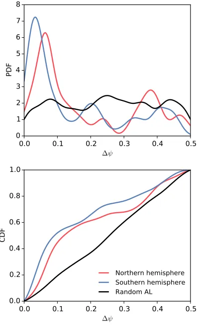
Fig. 6.— The upper/lower panel shows the PDF/CDF for CME occurrence. In the upper panel, the blue and red coloured lines are the PDF, obtained by KDE method, distinguished by the northern and southern hemispheres, respectively. The black line is from determining the PDF based on random-generated AL. In the lower panel, the CDFs of the above defined functions are shown.
sents a 1σstandard deviation of the sample along the re-gression line. The difference between the samples of two hemispheres is statistically insignificant, therefore the re-gression was applied to the data of both hemispheres. The obtained statistics suggests that there is a clear re-lationship between the tilt angle and the separateness parameter of the sunspot groups.
5. ENHANCED LONGITUDINAL BEHAVIOUR OF
CME EVENTS
5.1. Spatial probably CME occurrences
In this section, the connection between the CME oc-currence and AL is revealed. Panel Aof Figure6 shows the kernel probability density function of the longitu-dinal distribution of CME occurrence. This statistics is based on data from both the northern and southern hemi-spheres. There is only one significant peak visible around ∆ψ= 0.05. Besides this remarkable peak, there is a long plateau with some insignificant local peaks. Only one more peak, above the significance level at ∆ψ = 0.4, is present, but with a relatively weak activity when com-pered to the first peak.
A random-generated control group is also used in this statistic. The longitudinal position of AL now is a ran-dom position. This test was inspired by Pelt et al.
(2005) who expressed a critical view on the identifica-tion method of Berdyugina & Usoskin (2003) employed for AL. In our study, we applied the methodology intro-duced byPelt et al.(2005), who reconstructed the distri-bution of AL with random sunspot longitude data. The KDE plot of the control group does not show any peaks. This homogeneous distribution means that AL identifi-cation does not cause false significant peaks, which would affect the results.
PanelBof Figure6shows the cumulative distribution of the above-defined spatial distributions. The blue and red lines have a steep increasing phase between values of 0 and 0.1 followed by a less steep increasing trend. These results allow us to estimate that most of CMEs (around 60%) occur in a ±36◦ belt around the position of AL. Hence, the width of the longitudinal belt of CME occurrences is equal to the width of the longitudinal belt of solar flare occurrences (GY16). The black line is the cumulative distribution obtained from the analysis ap-plied to random longitudinal positions. This distribu-tion would only contain 20% of CMEs. This latter find-ing means that AL plays a significant role in the spatial distribution of CME occurrences.
5.2. CME dynamics
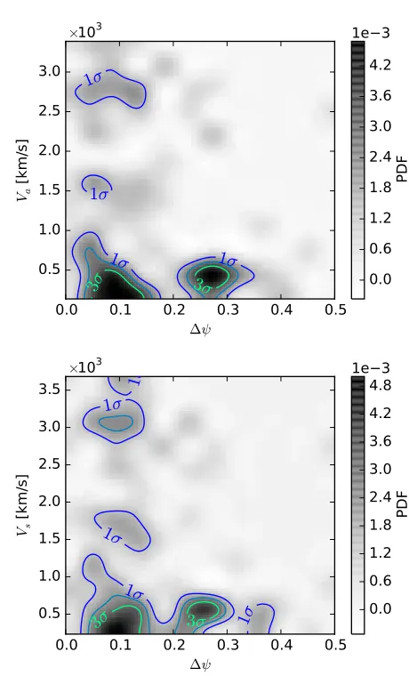
Let us now consider the apparent and space velocities (Va and Vs) of CME events. Two-dimensional kernel
density estimations are applied with an axis-aligned bi-variate Gaussian kernel, evaluated on a square grid of the ∆ψ−Va and ∆ψ−Vsspace. Figure7shows the result,
based on data from both hemispheres. The significance levels 1−3σare indicated by coloured contour lines.
[image:9.612.75.273.340.667.2]Active longitude and CME occurrences 9
0.0
0.1
0.2
0.3
0.4
0.5
∆ψ
0.5
1.0
1.5
2.0
2.5
3.0
Va
[k
m/
s]
×
10
31σ 1σ
1σ 1σ
3σ 3σ
0.0
0.6
1.2
1.8
2.4
3.0
3.6
4.2
1e 3
0.0
0.1
0.2
0.3
0.4
0.5
∆ψ
0.5
1.0
1.5
2.0
2.5
3.0
3.5
Vs
[km
/s]
×
10
31σ
1σ 1σ
1σ 1σ
3σ 3σ
0.0
0.6
1.2
1.8
2.4
3.0
3.6
4.2
4.8
1e 3
Fig. 7.—The result of the two-dimensional KDE, using parame-ters ∆ψandVa(apparent velocity of CME, upper panel),Vs(space velocity of CME, lower panel). The shade of the grey colour repre-sent the probability density. The significant islands are indicated by blue (1σ), dark green (2σ) and bright green (3σ) colours. The northern and souther hemispheres are not distinguished from each other.
Above the significance level of 3σ, there are only two islands. These are only slow CMEs inside and outside of AL. Analysis of this statistics also indicates that the probability of a slow CME is two standard deviation units higher than the probability that of a fast CME.
6. DISCUSSION
The AL identification method presented here reveals new spatial properties of the longitudinal distribution of the sunspot groups (PanelsD, E, F of the Fig 1). The spatial distribution of smaller sunspot groups (less then 1σ) is homogeneous. There is no enhanced longitudinal belt identifiable based on small sunspots; small groups appear everywhere as function of longitude. Moderate sunspot groups (between 1−2σ) show already inhomo-geneous properties. However, these results still have to be treated with caution. Only sunspot groups above the 3σ significance level have signatures of obvious and re-markable inhomogeneous spatial distribution.
The idea of two, almost equally significant longitudinal
zones is widely accepted by numerous studies, see e.g.
Berdyugina & Usoskin (2003). The dominant and
co-dominant active longitude is separated by 180 degrees
(Zhang et al. 2011b; Bumba et al. 2000). However, we
do not find such equally strong ALs (neither here nor in GY16). In our investigation, the co-dominant AL plays a less important role.
The spatial distribution of the separateness parameter (defined by Eq. 8) shows that complex active regions with a high CME capability appear near mostly the AL (Figure4). The appearance of moderate and simple com-plex configurations are everywhere on the solar surface. These groups are also able to have CMEs with a signifi-cantly lower probability.
We also found that, the most tilted sunspot groups have a complex configuration (Figure5). Simple bipolar sunspot groups show relatively small tilt angle. Saku-rai (2003) and Canfield (2012) concluded, that there is positive correlation between magnetic helicity and sunspot tilt angle. The sunspot rotation could play im-portant role in helicity transport across the photosphere. Sunspot rotation may increase helicity in the corona lead-ing to flares and CMEs (Pevtsov 2012). This property may also have the consequence of a more complex built-up of the underlying magnetic structure, and, the well-studied magnetic arches of the upper solar layer could be oriented at a large angle to the equator (Grigorev 2012). The more complex active regions are the more flares and they will be associated with CMEs (Huang et al. 2013;
Jetsu et al. 1997;Kitchatinov & Olemskoi 2005). Hence,
we conclude that the above physical process can take place within AL and anywhere else but only with low probability there.
Several studies have investigated east-west asymmetry of CMEs occurrence. Skirgiello(2007) found asymmetry using data provided by the SOHO-LASCO 1996−2004. The asymmetric behaviour could be a consequence of AL. Our result obtained here shows (see e.g. Fig7) that the number of CME occurrence is marginally higher within AL. The mean of the apparent and space velocity of CME occurrences is around 500 km/s considering the entire surface of the Sun. This mean velocity is known an ’slow’ CMEs, found in a number of earlier studies (Yinget al.
2016). However, the mean velocity is significantly higher if only the AL itself is considered. Within AL the average (or space) velocity is around 1000 km/s (see e.g.Michalek
et al. 2009). There is no fast CME occurrence found
outside of AL. Therefore, interestingly and notably, the fast HALO CMEs are also AL CMEs.
7. CONCLUSION
flare and CME source is predictable even several solar rotations in advance.
The observed properties of the non-axisymmetric solar activity need to be taken into account in developing and verifying suitable dynamo theory: the observations anal-ysed here show that there is only one significant AL with a relatively wide (±20−30 degrees) belt. Furthermore, the tilt angle of the active regions is also an important observed constraint for dynamo theory: the tilt angle of sunspot groups shows non-axisymmetric behaviour, which is a completely new (and surprising) finding.
ACKNOWLEDGMENTS
The results of this research was enabled partially by SunPy, an open-source and free community-developed Python solar data analysis package (Mumford et al.
2013). NG thanks for the support received from the University of Sheffield. NG also thanks for the labori-ous work done by the assistant fellows at Debrecen He-liophysical Observatory for composing the DPD sunspot catalog. RE acknowledges the support received by the Chinese Academy of Sciences Presidents International Fellowship Initiative, Grant No. 2016VMA045, the Sci-ence and Technology Facility Council (STFC), UK and Royal Society (UK).
REFERENCES
Bai, T., 1987, ApJ, 314, 795 Bai, T., 1988, ApJ, 328, 860 Bai, T., 2003a, ApJ, 585, 1114 Bai, T., 2003b, ApJ, 591, 406 Balthasar, H., 2007, A&A, 471, 281
Balthasar, H., Sch¨ussler, M., 1983, Solar Phys., 87, 23 Balthasar, H., Sch¨ussler, M., 1983, Solar Phys., 93, 177 Baranyi T. MNRAS, 2015
Becker, U., 1955, Z. Astrophys., 37, 47
Berdyugina, S.V., Usoskin, I.G., 2003, A&A, 405, 1121 Berdyugina, S.V., 2004, Solar Phys, 224, 123-131 Berdyugina, S.V., 2005, ASP Conference Series, 346
Berdyugina, S.V., Moss, D., Sokoloff, D.D., Usoskin, I.G.. Astron. Astrophys. 445, 703714, 2006.
Brouwer, M. P., Zwaan, C., 1990, Solar Phys. 129, 221 Bumba, V. et al. 1965, The Astrophys. J., 141, 14921517. Bogart, R.S.: 1982, Solar Phys. 76, 155 165.
Bornmann, P.L. & D. Shaw, V.I., 1994, Sol. Phys., 150, 127 Bumba, V., Obridko, V. N., 1969, Solar Phys., 6, 104
Bumba, V., Garcia, A., Klva˘na, M., 2000, Solar Phys., 196, 403 Carrington, R. C., 1863, Observations of the spots on the Sun
from November 9, 1853, to March 24, 1861 made at Redhill, Williams and Norgate, London,, Section VI, p. 246.
Castenmiller, M. J. M., Zwaan, C., van der Zalm, E. B. J., 1986, Solar Phys. 105, 237
Canfield, R. C., & Pevtsov, A. A. 1998, Sol. Phys., 182, 145 Chidambara, A. 1932, Mon. Not. R. Astron. Soc., 93, 150152. Cui, Y., Li, R., Zhang, L., He, Y., & Wang, H. 2006, SoPh, 237,
45
Colak, T. & Qahwaji R., 2008, Sol. Phys., 248, 277 Connolly, A. J., Genovese, C., Moore, A. W. Nichol,
R. C.,Schneider, J. and Wasserman, L., 2000, ArXiv Astrophysics e-prints,
http://adsabs.harvard.edu/abs/2000astro.ph..8187C
Gyenge, N., Baranyi, T., Ludm´any, A., 2014, Solar Phys., 289, 579 Gyenge, N., Baranyi, T., Ludm´any, A., 2016, ApJ, 818:127 (8pp) Gopalswamy, N.; Yashiro, S.; Michalek, G.; Stenborg, G.;
Vourlidas, A.; Freeland, S.; Howard, R., Earth, Moon, and Planets, Volume 104, Issue 1-4, pp. 295-313
N. Gopalswamy, H. Xie, S. Akiyama, P. Mkel, S. Yashiro, and G. Michalek ; The Astrophysical Journal Letters, 804:L23 (6pp), 2015 May 1 ; doi:10.1088/2041-8205/804/1/L23
Gosling, J.T., Hildner, E., MacQueen, R.M., Munro, R.H., Poland, A.I. & Ross, C.L., 1976, Sol. Phys., 48, 389 - 397 Grigorev, V., M., Ermakova, L., V. and Khlystova, A., I., 2012,
Astronomy Reports, 56, 878
Gy˝ori, L., Baranyi, T., Ludm´any, A. 2011, IAU Symp. 273, 403 Einbeck, J., Evers L., Bailer-Jones, C., Gorban, A., Kegl, B.,
Wunsch, D., Zinovyev A., Lecture Notes in Computational Science and Engineering, Springer, 2007, pp. 180–204 Hale, G. E., E., Ferdinand, Nicholson, S. B. & Joy, A. H. 1919,
ApJ, 49, p.153
Harrison, R.A., 1995, Astron. Astrophys., 304, 585 Henney, C. J., Durney, B. R., 2005, ASPC, 346, 381 Howard R., 1991b, Solar Phys., 136, 251
Howard, T. A. & Harrison, R. A. 2013, Sol. Phys., 285, 1-2, 269-280
Huang, X., Zhang, L., Wang, H., Li, L., 2013, A&A, 549, 127
Isobe T., Feigelson E. D., Akritas M. G., Babu G. J., 1990, ApJ, 364, 105
Ivanov, E. V., 2007, Adv. Spa. Res. 40, 959
Jetsu, L., Pohjolainen, S., Pelt, J., Tuominen, I., 1997, A&A, 318, 293
Juckett, D. A., 2006, Solar Phys., 245, 37 Juckett, D. A., 2007, Solar Phys., 245, 37
Kitchatinov, L. L., Olemskoi, S. V., 2005, Astron.Lett., 31, 280 Kiepenheuer, K.O., 1953, The University of Chicago Press, p.322 Kors´os, M., B., Ludm´any, A.; Baranyi, T. 2015, Apj, 789, 107 Kors´os, M., B., Ludm´any, A.; Erd´elyi, R.; Baranyi, T. 2015, Apj
Lett, 802, L21
Kors´os, M., B.; Erd´elyi, R.; 2016, Apj
Losh, H. M., 1939, Publ.Obs.Michigan, 7, no. 5., 127-145 Mason, J. P., & Hoeksema, J. T. 2010, ApJ, 723, 634 Maunder, E. W., 1905, MNRAS, 65, 538
McIntosh, P. S., 1990, Sol. Phys., 125, 251
Michalek, G.; Gopalswamy, N.; Yashiro, S., Sol. Phys., Volume 260, Issue 2, pp.401-406
Mumford, S.et al.2013, SunPy: Python for Solar Physicists, Proceedings of the 12th Python in Science Conference, 74-77. Obridko, V N; Chertoprud, V E; Ivanov, E V. Solar Physics,
272.1 (Aug 2011): 59-71.
Pelt, J., Tuominen, I., Brooke, J., 2005, A&A, 429, 1093 Pelt, J., Brooke, J. M., Korpi, M. J., Tuominen, I., 2006, A&A,
460, 875
Pevtsov A., Astrophysics and Space Science Proceedings, Volume 30. ISBN 978-3-642-29416-7. Springer-Verlag Berlin Heidelberg, 2012, p. 83-91
Sakurai, T. and Hagino, M., 2003. Journal of The Korean Astronomical Society, 36, 7-12
Schrijver, C. 2007, ApJL, 655, L117
Skirgiello, M. 2005, Annales Geophysicae, 23, 31393147
Usoskin, I. G., Berdyugina, S. V., Poutanen, J., 2005. A&A, 441, 347
I.G. Usoskin, S.V. Berdyugina, D. Moss, D.D. Sokoloff ,2007, Advances in Space Research 40. 951958
Waldmeier, M., 1938, Zeitschrift f¨ur Astrophysik, 16, 276 Waldmeier, M., 1947, Publ. Z¨urich, Band IX, Heft 1. Warwick, C. S., 1965, ApJ, 141, 500
Zhang, L.Y., Wang, H.N., Du, Z.L., Cui, Y. M., He, H., 2007, A&A, 471, 711
Zhang, L.Y., Wang, H.N., Du, Z.L., 2008, A&A,484, 523-527. Zhang, L.Y., Mursula, K., Usoskin, I. G., Wang, H.N., 2011,
A&A, 529, 23
Zhang, L.Y., Mursula, K., Usoskin, I. G., Wang, H.N., 2011, JASTP, 73. 258
Zhang, L.; Mursula, K.; Usoskin, I., 2015, A&A L., 575
Ester, M., H. P. Kriegel, J. Sander, and X. Xu, In Proceedings of the 2nd International Conference on Knowledge Discovery and Data Mining, Portland, OR, AAAI Press, pp. 226231. 1996 Warwick, C. S, 1966, ApJ, 145, 215
Xie, H., Ofman, L., Lawrence, G., Cone model for halo CMEs: Application to space weather forecasting, J. Geophys. Res., vol. 109, 2004, A03109.