Model structure selection using an integrated forward orthogonal search algorithm interfered with squared correlation and mutual information

This is a repository copy of

Model structure selection using an integrated forward

orthogonal search algorithm interfered with squared correlation and mutual information

.

White Rose Research Online URL for this paper:

http://eprints.whiterose.ac.uk/74558/

Monograph:

Wei, H.L. and Billings, S.A. (2006) Model structure selection using an integrated forward

orthogonal search algorithm interfered with squared correlation and mutual information.

Research Report. ACSE Research Report no. 918 . Automatic Control and Systems

Engineering, University of Sheffield

[email protected] https://eprints.whiterose.ac.uk/ Reuse

Unless indicated otherwise, fulltext items are protected by copyright with all rights reserved. The copyright exception in section 29 of the Copyright, Designs and Patents Act 1988 allows the making of a single copy solely for the purpose of non-commercial research or private study within the limits of fair dealing. The publisher or other rights-holder may allow further reproduction and re-use of this version - refer to the White Rose Research Online record for this item. Where records identify the publisher as the copyright holder, users can verify any specific terms of use on the publisher’s website.

Takedown

If you consider content in White Rose Research Online to be in breach of UK law, please notify us by

Model Structure Selection Using an Integrated Forward

Orthogonal Search Algorithm Interfered with Squared

Correlation and Mutual Information

H.L. Wei and S.A. Billings

Research Report No. 918

Department of Automatic Control and Systems Engineering

The University of Sheffield

Mappin Street, Sheffield,

S1 3JD, UK

Model Structure Selection Using an Integrated Forward

Orthogonal Search Algorithm Interfered with Squared

Correlation and Mutual Information

H. L. Wei and S.A. Billings

Department of Automatic Control and Systems Engineering, University of Sheffield Mappin Street, Sheffield, S1 3JD, UK

March 9, 2006

Model structure selection plays a key role in nonlinear system identification. The first step in nonlinear system identification is to determine which model terms should be included in the model. Once significant model terms have been determined, a model selection criterion can then be applied to select a suitable model subset. The well known orthogonal least squares type algorithms are one of the most efficient and commonly used techniques for model structure selection. However, it has been observed that the orthogonal least squares type algorithms may occasionally select incorrect model terms or yield a redundant model subset in the presence of particular noise structures or input signals. A very efficient integrated forward orthogonal searching (IFOS) algorithm, which is interfered with squared correlation and mutual information, and which incorporates a general cross-validation (GCV) criterion and hypothesis tests, is introduced to overcome these limitations in model structure selection.

Keywords: correlation, hypothesis tests, identification, model selection, mutual information,

NARX / NARMAX model.

1. Introduction

Model structure selection is the central task in nonlinear system identification. This topic, which

accompanies the development of system identification techniques, has been extensively studied in the

literature. In a broader sense, model structure selection is closely related to many practical themes

including data fitting, time series prediction, feature selection in classification, and complexity

reduction in neural networks. The conventional Akaike information criterion (AIC) (Akaike 1974), the

Bayesian information criterion (BIC) (Schwarz 1978), the minimum description length (MDL)

(Rissanen 1978), generalized cross-validation (GCV) (Golub et al. 1979), and many variants (Stoica et

al. 1986, Miller 1990, Haber and Unbehauen 1990, Stoica and Selen 2004) have been proposed to

determine the number of variables or regressors in the model, and this is often termed as model

selection or model order determination. Both parametric and nonparametric techniques have been

developed for variable selection (Hocking 1976, 1983, Breiman and Freedman 1983, Tjostheim and

(Montgomery et al. 2001, Stark and Fitzgerald 1995, Anders and Korn 1999, Lind and Ljung 2005)

have been studied for variable or regressor selection for some specific model structures. In network

modeling, mutual information (Battiti 1994, Zheng and Billings 1996), genetic algorithms (Mao and

Billings 1997), and robust regression and optimization methods (Hong and Harris 2002, 2002, Chen et

al. 2003, Hong and Chen 2005), have been introduced for network training. In order to increase the

robustness of a selected model for effectively handling ill-imposed problems (for example

multicollinearity) or to avoid undesirable overfitting, regularisation methods have been introduced to

interfere with the model structure detection procedure (Sjoberg and Ljung 1995, Orr 1995, Chen et al.

1996).

In nonlinear system identification and function (signal) approximation, model structure selection

often involves a great number of candidate model terms or basis functions. The first key step is to

determine which terms or bases are significant and should be included in the model. It is known that

inclusion of insignificant or redundant model terms might result in a much more complex model,

involving a large number of parameters, and as a consequence the model may become oversensitive to

training data and is likely to exhibit poor generalisation properties. For example, a redundant or

overfitted model may lack a satisfactory long term predictive capability. One of the main tasks in

nonlinear system identification therefore is to select a parsimonious model structure. Ideally, this

requires that the resulting model structure is optimal or at least suboptimal with regard to specified

modelling goals. Several approaches have been proposed to address this problem (Korenberg et al.

1988, Billings et al. 1988, Haber and Unbehauen 1990, Miller 1990, Mallat and Zhang 1993, David et

al. 1994). One of the most efficient and popular model structure detection techniques are the class of

orthogonal least squares (OLS) type algorithms (Korenberg et al. 1988, Billings et al. 1989, Chen et

al. 1989), which have been widely applied in nonlinear system identification. The orthogonal forward

regression (OFR) routine (Billings et al. 1989, Chen et al. 1989), which is one version of the OLS

algorithm, has a desirable advantage: the contributions of candidate model terms can be decoupled

and decomposed, and as a consequence the significance of each candidate model term can be

measured using the associated error reduction ratio (ERR). Significant model terms can thus be

ranked according to the ERR values. The order of selected model terms is independent of the order in

which the candidate model terms are progressively entered into the regression equation (Wei et al.

2004). The incorporation of the OFR-ERR type algorithms with other modelling techniques has

greatly raised the capability of improving the generalisation properties of the resulting models, see for

example, Aguirre and Billings (1994, 1995a, 1995b), Chen et al. (2003, 2005), and Billings and Wei

(2005a, 2005b).

It has been observed that the OFR-ERR type algorithms may occasionally select incorrect model

terms or yield a redundant model subset when either the training data are contaminated by certain

noise sequences (Mao and Billings), or the input is poorly designed, for example a second order low

system identification and any algorithm may fail to produce correct models in these worse case

scenarios. As will be seen later, however, the problems related to these cases can be avoided or

alleviated by inspecting and comparing the performance of a few models produced from some

trial-and-error tests. Piroddi and Spinelli (2003) proposed a promising approach to solve the model

structure selection problem by minimizing the simulation error, which is defined as the discrepancy

between the model predicted output and the measurements. However, the method of Piroddi and

Spinelli requires calculating model predicted outputs for all candidate model term combinations and is

thus time demanding. Mao and Billings (1997) proposed a solution to the combined problem of model

structure selection and parameter estimation by introducing a genetic searching algorithm, combined

with the standard orthogonal least squares routine. Although this requires much less calculations

compared with an optimal exhaustive search, the necessary computation is still quite large. In the

present study, a much simpler but efficient approach, which is easier to implement and quicker to

compute, for general nonlinear model structure selection, is proposed to solve the problem addressed

in Piroddi and Spinelli (2003) and in Mao and Billings (1997).

This study focuses on the model structure selection problem in nonlinear dynamical system

identification including model term detection and model subset selection. The main contributions of

the work include: i) a new criterion for measuring the significance of model terms is introduced based

on mutual information; the mutual information criterion can be used as a complementary approach or

an alternative to the ERR criterion; ii) a simple hypothesis test, based on the t-test, is introduced and

incorporated into the new orthogonal forward search algorithm; for linear-in-the-parameters models,

this kind of t-test provides an index to indicate which model terms are significant; iii) a new approach

is proposed for selecting an accurate model subset for a given identification problem. The squared

correlation and mutual information criteria, along with the t-tests and a general cross-validation (GCV)

criterion, are all incorporated into the new forward orthogonal search algorithm. For convenience, the

new integrated forward orthogonal search algorithm interfered with squared correlation and mutual

information will be referred to as the IFOS algorithm.

The remainder of the paper is organised as follows. In section 2 the orthogonal forward regression

(OFR) algorithm is briefly reviewed and the performance of this algorithm is discussed and analysed.

In section 3, the new integrated forward orthogonal search (IFOS) algorithm interfered with mutual

information is proposed. Four examples are described in section 4 to demonstrate the effectiveness and

applicability of the new IFOS algorithm. Some suggestions and discussions are included in section 5,

2. The OFR-ERR algorithm

In the following the discussion is restricted to models that can be expressed in a

linear-in-the-parameters form. This is an important class of representations for nonlinear system identification and

signal procession. Compared to nonlinear-in-the-parameters models, linear-in-the-parameters models

are simpler to analyse mathematically and quicker to compute numerically. The polynomial NARX

model will be used as an example to demonstrate the OFR-ERR algorithm. For the sake of

convenience in the descriptions, the two terms ‘system’ and ‘model’ will not be strictly distinguished

but the meanings of the two terms should be self-evident from the context.

2.1 The NARX model

The general form of the NARMAX (Nonlinear AutoRegressive Moving Average with eXogenous

inputs) model (Leontaritis and Billings 1985, Billings and Chen 1998, Pearson 1999, Piroddi and

Spinelli 2003) takes the form of the following nonlinear recursive difference equation:

y(t)= f(y(t−1),,y(t−ny),u(t−1),,u(t−nu),e(t−1),,e(t−ne))+e(t) (1)

where f is some unknown nonlinear mapping, u(t), y(t)ande(t) are the input, output, and the

prediction error,

n

n

n

polynomial function, model (1) can then be decomposed into a process related part and a noise related

part as

)) ( ( )) ( ( )

(t f t f t

y = p ϕp + n ϕn +e(t) (2)

where ϕp(t) =[y(t−1),, y(t−ny), u(t−1),,

T u n t

u( − )] is the process regressor vector, and

) (t n

ϕ =[y(t−1),, y(t−n_y), u(t−1),, u(t−nu),e(t−1),,e(t−ne)]T is the extended regressor

vector. The polynomial NARX (Nonlinear AutoRegressive with eXogenous inputs) model is a special

case of the polynomial NARMAX model, where the noise related model f reduces to a single noise n

term e(t) that can often be treated as an independent identical distributed (iid) zero mean noise

sequence providing that the function f pgives a sufficient description of the data set.

The polynomial NARX model can be expressed using a linear-in-the-parameters form

) ( ) ( )

( 1

t e t t

y M

m m m + =

∑

=

φ

θ (3)

whereφm(t)=φm(ϕ(t))are model terms generated in some way from the regressor vector ϕ(t)

, ), 1 (

[ − 

= y t y(t−ny), u(t−1),,

T u n t

u( − )] , θm are unknown parameters, and M is the total

form 1( ) ( )

1 t x t

xi i 

 , where xij(t)∈{y(t−1),,

j y(t−ny), u(t−1),, u(t−nu)} for j=1, 2, …,,

with 0≤ij ≤ and 0≤i1++i≤. The order of such a polynomial model is determined by n and y

u

n , and the nonlinear degree of such a model is referred to as.

2.2 The OFR-ERR algorithm

Consider the term selection problem for the linear-in-the-parameters model (3). Let

T N y y(1), , ( )]

[ 

=

y be a vector of measured outputs at N time instants, and m=[φm(1),,φm(N )]T be a vector formed by the mth candidate model term, where m=1,2, …, M. Let D={ 1,, M}be a

dictionary composed of the M candidate bases. From the viewpoint of practical modelling and

identification, the finite dimensional set D is often redundant. The model term selection problem is

equivalent to finding a full dimensional subset { , , } { , , }

1

1 n i i_n

n =  = 

D of n (n≤M)bases,

from the libraryD, where

k i

k = , ik∈{1,2,,M} and k=1,2, …, n, so that y can be satisfactorily

approximated using a linear combination of 1, 2,, n as below

e

y=θ_{1 1}++θ_{n n}+ (4)

or in a compact matrix form

e A

y= + (5)

where the matrixA=[ 1,, n] is assumed to be of full column rank,

T n] , , [θ1 θ

= is a parameter

vector, and e is the approximation error.

The model structure selection procedure starts from equation (3), with D={ 1,, M}. For

j=1,2,…, M, define

) )( (

) ( ] [ ERR

2 )

1 (

j T

j T

j T j

y y

y

= (6)

]} [ ERR { max

arg (1)

1

1 j

M j≤

≤

=

 (7)

The first significant basis can then be selected as

1

1=  , and the first associated orthogonal variable

can be chosen as

1

1 

q = .

Assume that a subsetDm−1, consisting of (m-1) significant bases, 1, 2,, m−1, has been

determined at step (m-1), and the (m-1) selected bases have been transformed into a new group of

orthogonalized bases q₁,q₂,,q_m−1via some orthogonal transformation. To select the mth significant

∑

−

= 1

1 )

(

m

k

k k T k

k T

j j

m

j q

q q

q

q (8)

] ) )[( (

) ( ]

[

ERR _{( ) ( )}

2 ) ( )

(

m j T m j T

m j T m

j

q q y y

q y

= (9)

where _j∈D−D_m−1. The mth significant basis can then be chosen as

m

m=  and the mth associated

orthogonal basis can be chosen as qm=q(m_m) , where argmax{ERR [ ]} ) (

1 j

m M

j m= _≤≤

 . Subsequent

significant bases can be selected in the same way step by step. At each step, the ‘best’ basis with the

strongest capability to represent the output y is selected. The selection procedure can be terminated

when some specified termination conditions are met.

The indices ERR(m)[j] are referred to as the error reduction ratios (ERR), and provide a simple

but effective means of selecting a subset of significant regressors. A more detailed explanation of ERR

can be found in Billings et al. (1989) and Chen et al. (1989).

Note that in many cases the noise signal e(t) in Eq. (3) may be a correlated or coloured noise

sequence. This is likely to be the case for most real data sets. The NARX model (3) will then become

the NARMAX model. For the NARMAX model, the structure selection procedure starts from

identifying the process NARX model, and the noise model can then be identified in the same way as

selecting the NARX model structure (Billings and Chen 1998). The inclusion of noise terms is mainly

used to reduce the bias in the parameters of the process NARX model.

2.3 The performance of the OFR-ERR algorithm

The OFR-ERR algorithm has been widely applied in model structure selection for nonlinear

system identification (Billings and Chen 1998) and has already become a standard algorithm for

nonlinear function approximation and neural network training (Haykin 1999, Nelles 2001, Harris et al.

2002). It has been observed, however, that this algorithm has some deficiencies when it is applied in

some worse case situations, where there are some uncertainties in the data or the input signal is not

very persistently exciting (Mao and Billings 1997, Piroddi and Spinelli 2003).

It has been observed that for some specific input signals, the model term y(t-1) is nearly always

selected as the first term with a very high ERR value, and as a consequence the contributions of other

model terms, measured by the associated ERR values, become small and are sensitive to the effect of

noise (Piroddi and Spinelli 2003). This problem seems to arise because of the input: a low order, low

frequency autoregressive (AR) process, though it is, by the standard definition for linear system

identification (Ljung 1987, Söderström and Stoica 1989), persistently exciting (of any finite order),

such an AR process as an input may not be sufficient for all ARX or NARX model identification. In

varying output signal. Assuming that the output signal, denoted by y(t), is sampled with at a fast

sampling rate (oversampled), the signal y(t) and the first few linear terms, y(t-1), y(t-2), …, will then

become strongly correlated and thus indistinguishable, implying that y(t)≈ y(t−1). This results

inERR(y,y1)≈1, where y andy are vectors formed by the output variable y(t) and the term y(t-1). 1 Consequently, the term y(t-1) is nearly always selected as the first term, regardless of whether the term

y(t-1) exists in the true model. The implication is that the type of input and the sampling regime may

affect the identification, irrespective of which particular algorithm is used.

The sampling interval for practical identification problem should therefore not be chosen to be too

small (Billings and Aguirre 1995). This is because too a small sampling interval may preclude

accurate structure selection for the following two reasons. Firstly, for a sufficiently small sampling

interval some candidate model terms will become indistinguishable, for example, the model terms

) 3 ( ) 2 ( ) 1

(t− y t− u t−

y , y2(t−1)u(t−1), y2(t−2)u(t−2), etc. may become equivalent to each other,

and the model selection criterion (ERR) may thus fail to distinguish between them. Secondly,

numerical problems will arise when the sampling time is chosen too small and such difficulties are

reflected in poor performance of the structure selection algorithm as shown in Billings and Aguirre

(1995).

Noise may also affect the model structure selection even when the training data are sampled with

an appropriate sampling rate. While all correct model terms ( ‘correct term’ here means that the term

exists in the original real model) can often be detected and included in the identified model, some

‘unnecessary’ (incorrect) model terms that do not exist in the original model may occasionally enter

into the selected model subset above some correct model terms. In most cases, nonlinear identification

is a structure-unknown problem. Almost all existing model structure selection algorithms are thus

data-oriented, that is, any algorithm will try to find a model structure that reflects as closely as

possible the information carried by observed noisy data (it is assumed that the data cannot be cleaned

by filtering), without any knowledge of the true model structure. Since realistically models must be

learned from noise contaminated data, spurious terms (incorrect terms) may also be included in the

identified model subset. However, a good model structure selection algorithm should be able to

provide a good model structure that minimizes the effects of incorrect (spurious) model terms to a

negligible level, such that the main underlying dynamics embodied in the data can be revealed or

captured by the identified model.

The effects of data uncertainty, the sample rate and the richness of the input signal on model

structure selection are genetic problems in all nonlinear system identification. The development of

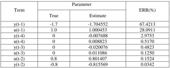
Table 1 Model selection results for Model I using the OFR-ERR algorithm

Term

Parameter

ERR(%) True Estimate

y(t-1) -1.7 -1.704552 67.4213

u(t-1) 1.0 1.000453 28.0911

y(t-4) 0 -0.007688 2.9753

u(t-4) 0 0.008823 0.5170

y(t-3) 0 -0.020076 0.4823

u(t-3) 0 0.011086 0.1250

u(t-2) 0.8 0.801407 0.1524

y(t-2) -0.8 -0.815569 0.0342

2.4 Two examples

Two simple examples will be used to illustrate some of the problems that arise if the training data

are contaminated by noise, or if the input is not sufficiently exciting. The two artificial examples are

given below:

Model I: y(t)=-1.7y(t-1)-0.8y(t-2)+u(t-1)+0.8u(t-2)+e(t) (10)

Model II: y(t)=0.7y(t−1)−0.1y(t−2)+u(t−1) (11)

The input u(t) in Model I is uniformly distributed on [-2,2], with the noise e(t)~N(0,0.12). The input

u(t) in Model II is a low frequency AR(2) process of the form: u(t)=1.6u(t-1)- 0.6375u(t-2)+ξ(t), with

) 1 , 0 ( ~ ) (t N

ξ . Note that although the AR(2) process is persistently exciting of almost any finite order,

it is a narrow band process behaving like a lowpass filter with minimum attenuation of low

frequencies nearω=0, with sharply increasing attenuation asω increases toward ω=π. This kind of

AR processes may not be sufficiently exciting for ARX and NARX model structure selection

(Leontaritis and Billings 1987).

One thousand input-output data points were generated from Model I. The candidate model terms

were set to be y(t-k) and u(t-k) where k=1,2,3,4,5. By applying the OFR-ERR algorithm to the given

10 candidate model terms, a model of 8 terms was produced as shown in Table 1, where the model

terms are ranked according to the order in which they were selected. It can be seen from Table 1 that

even though all the correct model terms were selected, the resulting model structure is not the

minimum or correct structure. The structure is a redundant model structure due to the inclusion of

some incorrect model terms. As will be seen later, all the incorrectly selected model terms can

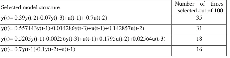
Table 2 Model selection results for Model II using the OFR-ERR algorithm

Selected model structure Number of times

selected out of 100 y(t)= 0.39y(t-2)-0.07y(t-3)+u(t-1)+ 0.7u(t-2) 35

y(t)= 0.557143y(t-1)-0.014286y(t-3)+u(t-1)+0.142857u(t-2) 31 y(t)= 0.5205y(t-1)-0.00256y(t-3)+u(t-1)+0.1795u(t-2)+0.02564u(t-3) 18

y(t)= 0.7y(t-1)-0.1y(t-2)+u(t-1) 16

Model II was simulated 100 times and at each time 1000 input-output data points were recorded.

By setting the candidate model terms to be the same as in Model I, the OFR-ERR algorithm was

applied over the 100 data sets respectively, and the model selection results are illustrated in Table 2,

where the model terms in each model structure are ranked according to the order that the terms were

selected. From Table 2, it can be seen that the true model structure was only correctly selected 16

times out of a 100 when the input signal was chosen to be a low frequency AR(2) process, even

though noise free data were used. These results suggest that the low frequency AR(2) input process is

so slowly varying that it is not sufficient exciting for ARX or NARX model structure identification.

An interesting phenomenon is that, although the 4 models given in Table 2 have different structures,

they all produce the same (in fact indistinguishable) model predicted or long term outputs for any

given input. Thus, in this regard, the four models are equivalent. It was also noticed that if the input

signal was set to a high frequency AR(2) process, say u(t)=0.6u(t-1)- 0.0875u(t-2)+ξ(t) with

) 1 , 0 ( ~ ) (t N

ξ , then the true model structure will be correctly identified.

As noted earlier, many factors can affect model structure selection including the presence of noise,

the sample rate and the richness of the input signal. Some subjective factors such as the selected

maximum lags in the input and output terms, and the nonlinear degree specified for nonlinear

candidate model terms will also affect the model structure selection. It has been verified by numerous

simulation examples that if the maximum lags or key variables of the system can be appropriately

chosen, then most of the irrelative model terms can be excluded and confidence of correctly selecting

a minimum model structure or nearly minimum model structure can be significantly increased. Thus

determining suitable values for the maximum lags and selecting significant variables as a first stage in

model structure selection is likely to be highly beneficial. In many cases, however, suitable maximum

lags and significant variables may be difficult to determine, and some alternatives are thus worthy of

3. The new IFOS algorithm

The above discussion suggests that there is a need to improve the OFR-ERR algorithm to try and

ensure that the correct model structure can be determined even when the data sets are not ideal. This

motivates the development of the new integrated forward orthogonal search (IFOS) algorithm

interfered with both the squared correlation and mutual information criteria. Before describing the

IFOS algorithm, some preliminaries will be described first.

3.1 Some definitions

Definition 1: Primary variables and derivative variables

A primary variable is a dependent variable that originally exists in the model which characterises a

given system. A derivative variable is derived from the primary variables. Generally, a primary

variable is explicit in the model, but a derivative variable is implicit.

Consider a model where there are three of primary dependent variables

y(t)= f(y(t−1),y(t−2),u(t−1)) (12)

The variables y(t−1),y(t−2),u(t−1) here are the primary dependent variables. Iterating (12) by one

step with respect to the primary variable y(t-1), yields

y(t)= f(y(t−1),y(t−2),u(t−1))

= f(f(y(t−2),y(t−3),u(t−2)),y(t−2),u(t−1)) (13)

The induced model (13) now involves 4 variablesy(t−2),y(t−3), u(t−1)and u(t−2), where y(t-3)

and u(t-2) are derived variables. Inspection of the results in Table 1 for Model 1 in section 2.4 shows

that, some of the derived variables may have been induced by the presence of noise if the candidate

maximum lags are set to be too high. Therefore, if the primary variables of the system can be

determined initially from the observational data, the accuracy of the model structure selection can then

be significantly improved. Notice that the non-uniqueness which produces the result that the models in

Eqs. (12) and (13) are equivalent is a direct result of the discrete model form and not the structure

selection algorithm.

Definition 2: Model term dictionary

A model term dictionaryD is a set whose elements are some specified (candidate) model terms

(also called atoms or bases in signal procession). A dictionary D is said to be over-complete if all the

true model terms are included inD . A dictionary D is said to be under-complete (or incomplete) if at

least one true model term is not included inD . A dictionary Dis said to be exactly-complete if all the

exactly-complete dictionary the identification problem reduces to a structure-known estimation

problem.

Assume that a system is described by the model:y(t)=0.7y(t−1)−0.1y(t−2)+u(t−1) , then

)} 2 ( ), 1 ( ), 2 ( ), 1 ( {

1= y t− y t− u t− u t−

D is over-complete; D2 = {y(t−1), y(t−1)u(t−1), u(t−2)} is

under-complete; and D₃= {y(t−1),y(t−2),u(t−1)}is exactly-complete.

For a NARX model with a nonlinear degree and maximum lags n (for output) and y n (for u

input), the candidate model term dictionary, including the constant term, is

} 0 , 0 , 1 , : ) ( ) (

{ _{1 , 1 1}

,

, = x1 t x t x ∈ n n ≤ j≤ ≤ij≤ ≤i ++i ≤ i

j i i

n

n y u

j u

y V

D (14)

where _, ={y(t−1),, u

y n n

V y(t−ny), u(t−1),, u(t−nu)}. The number of elements in the dictionary

 , , _u y n n

D is _  [( y u )!]/[( y u)!!] n n n n n n

C y+ u+ = + + +

.

Definition 3: Model library

A model libraryL is a set whose elements are some specified models. A model selection criterion

is always performed over a given model library.

Given a model libraryL , the objective of model selection is to find the ‘best’ model from the

library. All model selection criteria are relative, and there exists no absolute criterion that is able to

measure all model fits under all conditions. A criterion will select the ‘best’ model structure over all

the others even when the model library is inadequate (‘inadequate’ here means that no models in the

library are exactly correct but only approximately correct). With regard to what the ‘best’ model is,

this depends on the specific situation. For example, the first three models given in Table 2 are

structure incorrect compared with the true model. However, all the four models are equivalent if the

model predicted outputs are used as the criterion. The ‘correctness’ of a model structure is thus always

relative.

Definition 4: Model behaviour equivalence

Two modelsM₁ and M₂ are said to be equivalent with each other in behaviour, if the (model

predicted) outputs of the two models, driven by the same input, are the same. In practice, it may be

impossible to get exactly the same output behaviour for two different models. Thus, two modelsM₁

and M2 are often considered approximately equivalent when their outputs are sufficiently close.

Assume that an identified model,M, is given by

)) ( , ), 1 ( ), ( , ), 1 ( ( )

(t f y t y t ny u t y t nu

y = −  − −  − +e(t) (15)

At a given time instancet , setting ₀ yˆmpo(t₀−k)=y(t₀−k) for k=1,2, …, n , model predicted outputs _y

= ) ( ˆ t

ympo yˆmpo(t,M)= (ˆ ( 1), ,ˆ ( y), ( 1), , ( u)) mpo mpo n t u t u n t y t y

f −  − −  − (16)

While one-step-ahead predictions are often used to validate an identified model, previous

experience shows that even a poor (e.g., insufficient, biased, unstable, etc.) model can provide good

one-step-ahead predictions. Model predicted outputs can reveal severe model deficiencies which

would otherwise go undetected by one-step-ahead predictions. However, in some cases, model

predicted outputs may be unstable or may decay to zero, implying that model predicted outputs

become invalid. In this case, a trade-off between one-step-ahead predictions and model predicted

outputs is to use multi-step-ahead predictions.

Multi-step-ahead predictions, for example m-step-ahead predictions, can be calculated in an

iterative way. At a given time instancet , setting ₀ yˆmsa(t₀−k)=y(t₀−k) for k=1,2, …, m-1;

m-step-ahead predictions at time instancest≥t₀ can be obtained by calculating the two stages alternatively as

below:

Stage 1: Prediction:

= ) ( ˆ t

ymsa yˆmsa(t,M)

)) ( , ), 1 ( ), ( ), ( ), 1 ( ˆ , ), 1 ( ˆ

( y u

msa msa n t u t u n t y m t y m t y t y

f − − + − − − −

=   (17a)

) ( ˆ ) (

ˆ t y t

ytemp = msa (17b)

Stage 2: Updating:

   + − − + − = + − otherwise. ), 1 ( ˆ , of multiple is ), 1 ( ) 1 ( ˆ 0 m t y m t t m t y m t

ymsa _temp (17c)

3.2 Model term selection interfered with squared correlation and mutual information

3.2.1 Squared correlation coefficient

The Pearson correlation coefficient is a frequently used function. The standard correlation

coefficient between two N-dimensional random vectors x and y is defined as r( yx, )=

) var( ) var( / ) ,

cov(x y x y , where cov(⋅) designates the covariance and var(⋅) the variance. Using this definition, an estimate of the standard correlation coefficient can be calculated based on centralized

data; the estimate is given by

∑

∑

∑

i i i

y y x x y y x x r 1 2 1 2 1 ) ( ) ( ) )( ( ) ,

( yx (18a)

where x and y are the mean values of x and y. Notice that in many cases data centralisation may be

non-centralised squared correlation coefficient, which is also known as the squared correlation value

between x and y, is defined as

∑

∑

∑

2 _{( )}

) )( ( ) ( ) , ( y y x x y x y

x (18b)

Note that the ERR criterion in the OFR-ERR algorithm described in section 2.2 is equivalent to the

non-centralized squared correlation function (18b). This function is also employed as the selection

criterion in the matching pursuit orthogonal least squares algorithm (Wei and Billings 2005).

3.2.2 Mutual information

Mutual information has now been extensively studied in the literature and applied to various areas.

Following Cover and Thomas (1991), mutual information is defined as follows.

Consider two random discrete variables x and y with alphabet X andY, respectively, and with a

joint probability mass function p(x, y) and marginal probability mass functions p(x)andp( y). The

mutual information I( yx, ) is the relative entropy between the joint distribution and the product distributionp(x)p(y), given as

            = ) ( ) ( ) , ( log ) , ( y x y x y x p p p E I       =

∑∑

(19)

The mutual informationI( yx, )is the reduction in the uncertainty of y due to the knowledge of x, and vice versa. Mutual information provides a measure of the amount of information that one variable

shares with another one. If y is chosen to be the system output (the response), and x is one regressor in

a linear model, I( yx, )can be used to measure the coherency of x with y in the model.

3.2.3 Interference of mutual information in model structure selection

Mutual information can easily be incorporated into the orthogonalization procedure in the same

way as the squared correlation coefficient. Let D ={ _j:j=1≤ j≤M}be a given model term

dictionary. Let r0 =y, and

)} , ( { max arg 0 1 1 j M j≤ I r

≤

=

 (20)

where I(⋅,⋅)is the mutual information function given by (19). The first significant basis can thus be

selected as

1

1 1 1 1 0 0 1 q q q q r r r _T T −

= (21)

At the second step, let 1 1 1 1 ) 2 ( )] /( )

[( q q q q

qj = j− Tj T , where j∈D

and

. D

)} , ( { max

arg ₁ (2) 2

1

j j  I r q



≠

= (22)

The second significant basis can thus be chosen as

2

2 =  , and the second associated orthogonal

basis can be chosen as q2=q(2₂). Set

2 2 2 2 1 1 2 q q q q r r r _T T −

= (23)

In general, the mth significant model term can be chosen as follows. Assume that at the (m-1)th

step, a subsetDm−1, consisting of (m-1) significant bases, 1, 2,, m−1, has been determined, and the

(m-1) selected bases have been transformed into a new group of orthogonal bases q₁,q₂,,q_m−1via some orthogonal transformation. Let

1 1 1 1 2 2 1 − − − − − −

− = − m

m T m m T m m m q q q q r r

r (24)

∑

q (25)

)} , ( { max

arg 1 ( )

1 1 , m j m m k j m I k q r ₋ − ≤ ≤ ≠ = 

 (26)

where _j∈D−D_m−1. The mth significant basis can then be chosen as

m

m=  and the mth associated

orthogonal basis can be chosen as qm=q(m_m). Subsequent significant bases can be selected in the same

way step by step.

From (24), the vectors rm−1and qm−1 are orthogonal, thus

1 1 2 1 2 2 2 2 1 ) ( || || || || − − − − − − = − m T m m T m m m q q q r r

r (27)

By respectively summing (24) and (27) for m from 2 to n+1, yields

n n m m m T m m T

m _{q r}

q q q r y

∑

1 ₍₂₈₎

∑

2 ( )

|| || || || q q q r y

The residual sum of squares, also called the sum-squared-error, ||rn||2, or its variants including the

mean-square-error (MSE) or the error-to-signal ratio defined as ||rn||2 ||y||2 , can be used to form criteria for model selection. The model term selection procedure can be terminated when some

specified termination conditions are met.

The motivation for introducing the mutual information interfered criterion here is not to totally

replace the commonly used ERR criterion, but rather to provide an alternative and complementary

approach to the ERR criterion. Further details will be given in Section 4.

3.2.4 Parameter estimation

It is easy to verify that the relationship between the selected original bases ₁, ₂,, _m, and the

associated orthogonal basesq₁,q₂,,q_m, is given by

m m m Q R

A = (30) where R is an m m×munit upper triangular matrix whose entries uij(1≤i≤ j≤m) are calculated

during the orthogonalization procedure, and Qm is an N×m matrix with orthogonal

columnsq₁,q₂,,q_m. The unknown parameter vector, denoted by m=[θ1,θ2,,θm]T, for the model with respect the original bases (similar to (4)), can be calculated from the triangular equation

m m m g

R = withgm=[g1,g2,,gm]T , where ( 1 )/( k) T k k T k k

g = r ₋q q q or ( )/( k) T k k T k

g = y q q q .

Note that some tricks can be used to avoid selecting strongly correlated model terms. Assume that

at the mth step, a subsetDm, consisting of m significant bases, 1, 2,, m, has been determined.

Also assume that _j∈D−D_mis strongly correlated with some bases in D_m, that is, _j is a linear

combination of 1, 2,, m. Thus there exist m real numbersk1,k2,,km, at least one of which is

different from zero, such that

m m

j=k1 1+k2 2+k (31)

From (30), there exists another set of real numbers, µ₁,µ₂,,µ_m, such that

m m

j =µ1q1+µ2q2+µ q (32)

For the candidate basis given by (32), equation (25) becomes

0 q q q

q q = −

∑

−

=

1

1 )

(

m

k

k k T k

k T

j j

m

j (33)

Therefore, ( ( )) (jm) =0 T

m j q

In the IOFS algorithm, the candidate basis _j∈D−D_m will be automatically discarded if } , 1 { 10 )

( ( ) ( ) j

T j m j T m j q

q < −τ , where τ is a positive number that is large enough. In this way, any severe

mullticolinearity or ill-conditioning can be avoided.

3.3 Model order determination

The role of model order determination in dynamical system identification has been widely

recognised and various model selection criteria have been well established, see for example the recent

review paper by Stoica and Selen (2004). Model selection criteria are often established on the basis of

estimates of prediction errors, by inspecting how the identified model performs on future (never used)

data sets.

One general routine for model selection, which tries to avoid or reduce any possible bias

introduced by relying on any particular test data sets, is cross validation (Stone 1974). Cross-validation

has a number of variations, two commonly used variants of which are the leave-one-out (LOO), also

called predicted sum of squares (PRESS) (Allen 1974), and generalised cross-validation (GCV)

(Golub et al. 1979). Generalised cross-validation, due to its convenience of use and effectiveness for

avoiding overfitting, has been widely accepted.

Now consider the model (28) obtained in the m-th search step. Notice that the inner product term

m T m q

r −1 in this model can be replaced by m T

q

y

.

The penalised algorithm is based on the following minimisation criterion

∑

(M ,g,λ) r r λ m

T m m T

mr g g

r +λ

= (34)

whereλis the regularisation parameter. The solution to the above ridge regression is

y Q I Q Q

g m m Tm T m m 1 ) ( + −

= λ (35)

and the minimised error (energy) is

y P y m

T m

E = (36)

where m m Tm

T m m m

m I Q Q Q I Q

P = − ( +λ )−1 , andI is the m-dimensional identity matrix. Following m Golub et al. (1979) and Orr (1995), GCV is given by

2 2 GCV )) trace( ) / 1 (( 1 ) , ( m m T m N N m P y P y = M O N N N m T m y P y 2 2       − =

whereγ_mis the effective number of parameters (Moody 1992). Clearly, if λ=0, (37) reduces to the

ordinary GCV criterion with γm=m and m T m m T m T r r y P y y P

y 2 = = . For the general case in ridge regression, whereλ≠0, it can be shown that

      + + + − − =

∑

O (38)

where q₁,q₂,,q_m are the columns of the matrixQ , and the effective number m γmis calculated to be

∑

1 q q

q q

λ

γ (39)

It has been suggested (Orr 1998) that the regulation parameterλ should be determined based on

GCV minimisation, and the formula for updatingλfor the identified model with m terms is given as

m T m m T m

N g V g

r r 1 − − = γ η

λ (40)

where ( m m)

T

mQ I

Q

V= +λ , η=trace(V−1−λV−2). Other simple updating formula are also available (Chen et al. 1996, Billings and Chen 1998)

m T m m T m m m m

N g g

r r new new new γ γ λ −

= (41)

whereγ is given by (39).

3.4 Hypothesis tests on individual regression coefficients

Statistical methods play a unique role in the diagnosis and analysis of linear models. One aspect of

the application of statistical methods for linear model analysis is hypothesis tests on regression

coefficients (Hocking 1976, 1983, Montgomery et al. 2001). Consider the linear regression model

with k regressors below

e X

y= + (42)

where y is N×1, X is N×n( all the elements of the first column of X are assume to be unit), is

1 ×

n , e is n×1, and n=k+1. A frequently asked question is: do all the k regressors contribute

significantly to the regression model?

To inspect whether some subset of r < k regressors contribute significantly to the regression model,

let the design matrix X be sub-divided into two parts as X=[X1,X2], and the parameter vector be

partitioned as =[ ₁T, ₂T]T, accordingly, where X is ₁ N×(n−r), X is ₂ N×r, ₁is (n−r)×1, and

e X X

y= 1 1+ 2 2+ (43)

The objective now is to test the hypotheses

0

= 2 0:

H (44a)

0

≠ 2 1:

H (44b)

Montgomery et al. (2001) suggested that the null hypothesis H0: 2 =0 may be tested by the statistic

s MS SS SS r F Re 1 R R 0 )] ( ) ( )[ / 1 ( −

= (45)

where SSR( )=yTHy , R( 1) y H1y T

SS = , MSRe ( ) /(N n)

T

s=y I−H y − , and

T T X X X X

H= ( )−1 ,

T T 1 1 1 1 1

1 X(X X ) X

H = − .

For a given α , whereα is a small positive number such that (1−α)×100% indicates the

confidence interval, if F0>Fα,r,N−n, the H0: 2 =0 can then be rejected, concluding that at least one

of the parameters in 2in not zero, and consequently at least one of the regressors in X contributes 2 significantly to the regression model. The test given in (45) is also called a partial F-test because it

measures the contribution of the regressors in X given that the other regressors in 2 X are already in 1 the model. See Montgomery et al. (2001) for details about the partial F-test and other hypothesis tests.

The simplest but useful hypothesis for testing the significance of any individual regression

coefficient, for instance j in the model (42), is

0 : 0 j =

H (46a)

0 : 1 j ≠

H (46b)

If there is no sufficient reason to reject the null hypothesisH₀: _j =0, then the corresponding

regressorx can be removed from the model. The test statistic for this hypothesis is j

) ˆ se( | ˆ | 0 j j t θ θ

= (47)

where se(θˆj)= σˆ2c*jj is the standard error of the regression coefficient j , *

jj

c is the diagonal

element of (XTX)−1 corresponding to ˆ , and _j σˆ2=MS_Resis the unbiased estimator of variance.

For a givenα, if t0>tα/2,N−n, the null hypothesisH0: j =0 can then be rejected. Note that this is

really a partial or marginal test (Montgomery et al. 2001) because the regression coefficient

j

ˆ depends on all of the other regressors that are in the model. Thus it is a test of the contribution of

j

x given the other regressors in the model. Clearly, the t-test in (47) is a special case of the F-test in

For practical identification problems, whereN−n>120, tα/2,N−n ≈1.96ifα is set to 0.05, an

equivalent test to (47) is

) ˆ se( 96 . 1

| ˆ | 0

j j t

θ θ

= (48)

If t0>1, the null hypothesisH0: j =0 can then be rejected.

4. Case studies

In this section, several examples are provided to illustrate how to select an accurate model

structure using the new IFOS algorithm. It will be shown that the IFOS algorithm can detect spurious

model terms even when the data are contaminated with noise. A spurious model term here means that

the model term is not in the true model but is selected with an ERR value that is not small. For cases

where the input is not sufficiently exciting, a trial-and-error approach can be used to avoid selecting

the terms y(t-1), y(t-2), etc., providing that these terms are not in the true model.

Notice that in the given examples, both artificial models and real data sets, where it is believed to

be difficult to find the correct model structure, have been deliberately chosen to illustrate the

effectiveness of the new IFOS algorithm.

The IFOS algorithm interfered with squared correlation will be referred to as IFOS-SC. Similarly,

the mutual information interfered IFOS, will be referred to as IFOS-MI.

4.1 Example 1—the input is white

The following model was taken from Mao and Billings (1997)

) 2 ( 5 . 0 )

(t =− y t−

y +0.7y(t−1)u(t−1) +0.6u2(t−2)

) 1 ( 2 . 0 3 −

+ y t −0.7y(t−2)u2(t−2) +e(t) (49)

where the input u(t) was uniformly distributed on [-1, 1], with the noise e(t)~N(0,0.022). Following

Mao and Billings (1997), the maximum lags of both the input and the output were assumed to be 4 and

the nonlinear degree to be 3. Five hundred input-output data were generated and were used for model

structure selection. The new IFOS algorithm, which incorporates the t-test given by (48), was applied

to the data set, and the results are shown in Tables 3 and 4.

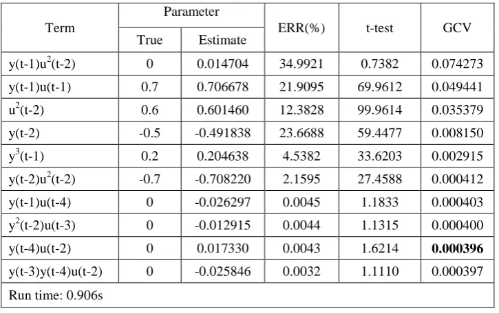
From Table 3, the ERR values show that the first 6 model terms are significant and should be

included in the model. The first selected term, y(t-1)u2(t-2), with the highest ERR value is spurious.

The t-tests show that among all the 10 model terms selected with the ERR criterion, only 5 are

significant and the t-tests of the 5 terms are significantly different from unity. This means that the 5

terms with the highest t-tests dominate the regression model. This can easily be confirmed by

Table 3 Identified model structure for system (49) using the IFOS-SC algorithm

Term

Parameter

ERR(%) t-test GCV True Estimate

y(t-1)u2(t-2) 0 0.014704 34.9921 0.7382 0.074273 y(t-1)u(t-1) 0.7 0.706678 21.9095 69.9612 0.049441 u2(t-2) 0.6 0.601460 12.3828 99.9614 0.035379 y(t-2) -0.5 -0.491838 23.6688 59.4477 0.008150 y3(t-1) 0.2 0.204638 4.5382 33.6203 0.002915 y(t-2)u2(t-2) -0.7 -0.708220 2.1595 27.4588 0.000412 y(t-1)u(t-4) 0 -0.026297 0.0045 1.1833 0.000403 y2(t-2)u(t-3) 0 -0.012915 0.0044 1.1315 0.000400 y(t-4)u(t-2) 0 0.017330 0.0043 1.6214 0.000396

y(t-3)y(t-4)u(t-2) 0 -0.025846 0.0032 1.1110 0.000397 Run time: 0.906s

Table 4 Identified model structure for system (49) using the IFOS-MI algorithm

Term

Parameter _Mutual

Info t-test GCV True Estimate

y(t-2)u2(t-2) -0.7 -0.690247 0.251193 42.2583 0.118617 u2(t-2) 0.6 0.599793 0.320914 149.1860 0.048510 y(t-1)u(t-1) 0.7 0.705487 0.188335 99.3864 0.026045 y(t-2) -0.5 -0.501902 0.227581 66.5005 0.014168 y3(t-1) 0.2 0.201394 0.214758 65.9884 0.000393

u2(t-1)u(t-4) 0 -0.002367 0.012226 0.3664 0.000394 u2(t-2)u(t-3) 0 -0.001729 0.008698 0.2627 0.000396

values show that the appropriate number of model terms is 9, but clearly a model of 9 terms is

overfitted.

Compared with Table 3, results given in Table 4 are quite optimistic. The t-tests show that only 5

model terms are significant, and the five model terms are exactly consistent with the 5 true model

terms. In addition, GCV provides a correct indication of the structure, suggesting that 5 model terms

are appropriate. Thus, from the results given by Table 3 and 4, all model terms can be correctly

4.2 Example 2—the input is non-white

Consider the following two systems

1

S : w(t)=0.5w(t−1)+0.8u(t−2) +u2(t−1)−0.05w2(t−2)+0.5 (50a)

) ( 5 . 0 1

1 )

( )

( t

q t

w t

y _−qξ

− +

= , ξ(t)~N(0,0.052) (50b)

2

S : w(t)=u(t−1)+0.5u(t−2) +25u(t−1)u(t−2)−0.3u3(t−1) (51a)

) ( 8 . 0 1

1 )

( )

( t

q t

w t

y _−qξ

− +

= , ξ(t)~N(0,0.022) (51b)

Following Piroddi and Spinelli (2003), the input u(t) to the two systems were chosen as a low

frequency AR(2) process of the form: u(t)=1.6u(t-1)-0.6375u(t-2)+0.16ζ(t), with ζ(t)~N(0,1). Two

data sets of 500 input-output samples were generated from each system and the two data sets were

used for model structure selection.

4.2.1 Experiments for system S₁

Following Piroddi and Spinelli (2003), the maximum lags of both the input and the output were

assumed to be 2 and the degree of nonlinearity to be 2. Model structure selection results for system

1

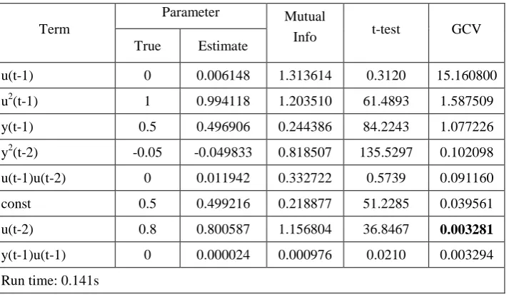
S are reported in Tables 5 and 6. Following the analysis in Example 1, it is clear that the significant

model terms should be selected as y(t-1), u(t-2), u2(t-1), y2(t-2), and the const term, which are exactly

the same as the true model. Note that once the 5 model terms have been determined, the parameters

Table 5 Identified model structure for the system (50) using the IFOS-SC algorithm

Term

Parameter

ERR(%) t-test GCV True Estimate

y(t-1) 0.5 0.500106 91.1027 71.4985 1.511037 y2(t-2) -0.05 -0.049757 3.5098 128.3416 0.922388 u2(t-1) 1 1.000401 2.0742 132.8120 0.571884 u(t-2) 0.8 0.806721 2.8537 125.5270 0.079973 const 0.5 0.493459 0.4406 43.4106 0.003336

y2(t-1) 0 -0.000419 0.0001 0.8359 0.003343 u2(t-2) 0 0.006367 0.0001 0.6223 0.003360 Run time: 0.032s

Table 6 Identified model structure for the system (50) using the IFOS-MI algorithm

Term

Parameter _Mutual

Info t-test GCV True Estimate

u(t-1) 0 0.006148 1.313614 0.3120 15.160800 u2(t-1) 1 0.994118 1.203510 61.4893 1.587509 y(t-1) 0.5 0.496906 0.244386 84.2243 1.077226 y2(t-2) -0.05 -0.049833 0.818507 135.5297 0.102098 u(t-1)u(t-2) 0 0.011942 0.332722 0.5739 0.091160 const 0.5 0.499216 0.218877 51.2285 0.039561 u(t-2) 0.8 0.800587 1.156804 36.8467 0.003281

y(t-1)u(t-1) 0 0.000024 0.000976 0.0210 0.003294 Run time: 0.141s

4.2.2 Experiments for system S₂

Following Piroddi and Spinelli (2003), the maximum lags of both the input and the output were

assumed to be 2 and the degree of nonlinearity to be 3. To ensure selection of the correct model

subset, the IFOS-SC algorithm was applied over the following 5 different candidate model term

dictionaries:

3 , 2 , 0 D

Du = , 2,2,3 0

)} 1 ( { 0

1_{= − −}

t y D

D ,

)} 2 ( { 0

2_{= − −}

t y D

D ,

)} 2 ( ), 1 ( { 0

3_{= − − −}

t y t y D

D ,

where the model term dictionary _{, ,} u y n n

D was defined by (14). The reason that the 5 different

candidate dictionaries were considered here was to avoid selecting the terms y(t-1) and y(t-2),

providing that these terms were not in the true model. Five different models, corresponding to the 5

dictionaries, were selected and the identified models are shown in Table 7. Similar results were also

obtained using the IFOS-SC algorithm, but to save space the results are not shown here.

While it is not quite apparent which model terms should be included in the model from the results

with respect to D0and D2, it is quite clear from the results with regard to Du, D1and D3 that the

significant model terms included in the model should be u(t-1), u(t-2), u(t-1)u(t-2), and u3(t-1), which

are exactly the same as required by the system. Note that the search time to select the model terms is

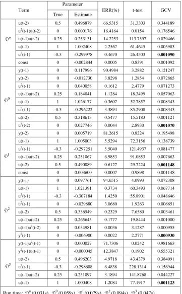
Table 7 Identified model structures for the system (51) using the IFOS-SC algorithm

Term

Parameter

ERR(%) t-test GCV True Estimate

u D

u(t-2) 0.5 0.496879 66.5315 31.3303 0.344189

u2_{(t-1)u(t-2) 0 0.000176 16.4164 0.0154 0.176546}

u(t-1)u(t-2) 0.25 0.253131 14.2253 113.7397 0.029466

u(t-1) 1 1.002408 2.2567 61.4645 0.005983

u3(t-1) -0.3 -0.299978 0.4670 26.4503 0.001090

const 0 -0.002844 0.0005 0.8391 0.001092

0 D

y(t-1) 0 0.117996 90.4984 3.2882 0.121247

y(t-2) 0 -0.012730 3.8298 1.2854 0.072865

u2(t-1) 0 0.040058 0.1612 2.4779 0.071273

u(t-1)u(t-2) 0.25 0.184041 1.1284 18.3499 0.057063

u(t-1) 1 1.026177 0.3607 52.7857 0.008343

u3(t-1) -0.3 -0.296222 3.3894 85.2908 0.008343

u(t-2) 0.5 0.318613 0.5477 15.5183 0.001121

u3(t-2) 0 0.027746 0.0044 2.8930 0.001070

1 D

y(t-2) 0 0.005719 81.2615 0.8224 0.195498

u(t-1) 1 1.005003 5.5294 72.3156 0.138739

u3(t-1) -0.3 -0.297251 5.5040 121.4937 0.081477

u(t-1)u(t-2) 0.25 0.251067 6.9853 91.0853 0.007663

u(t-2) 0.5 0.490089 0.6127 29.7224 0.001148

const 0 0.003600 0.0007 0.9898 0.001148

2 D

y(t-1) 0 0.097761 94.6515 4.0993 0.072308

u(t-1) 1 1.021391 0.3734 60.3493 0.067714

u3(t-1) -0.3 -0.307184 1.4250 55.8901 0.048646

u2(t-1) 0 -0.029880 3.0680 1.9263 0.006651

u(t-2) 0.5 0.336549 0.2329 7.6580 0.003461

u(t-1)u(t-2) 0.25 0.265645 0.1777 19.8444 0.001000

u(t-1)u2(t-2) 0 0.034981 0.0036 3.1287 0.000955

y2(t-1) 0 -0.006900 0.0022 2.2771 0.000930

3 D

y(t-1)u2(t-1) 0 0.000027 71.7306 0.0242 0.981663

y2(t-1)u(t-1) 0 -0.000045 12.3847 0.1902 0.555321

u(t-2) 0.5 0.496203 4.9718 43.4379 0.384091

u3(t-1) -0.3 -0.298608 6.4838 228.1314 0.156944

u(t-1)u(t-2) 0.25 0.251097 3.1894 141.8768 0.044227

u(t-1) 1 1.000408 1.2084 77.1917 0.001123

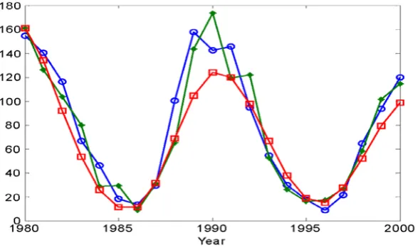
4.3 Example 3—forecasting annual sunspot numbers

The data set used in this example contains 301 observations of the annual sunspot numbers from

1700 to 2000. The first 280 samples for years 1700 to 1979 were used for model identification and the

remaining 22 data were used for model performance testing. The candidate model term dictionaries

were chosen as D0=D_12,0,1={y(t−1),, y(t−12)}, and D1=D0-{y(t-1),y(t-2)}. The reason that the

maximum lag was chosen to be 12 is due to the fact that the annual sunspot time series has a cycle that

is about 11years. A nonlinear model for the sunspot time series may be more appropriate, the objective

in this example, however, is to illustrate the efficiency of the new IFOS algorithm for model structure

selection, and a linear model was thus adopted.

The selected model structures from the dictionary D0using both IFOS-SC and IFOS-MI are shown

in Table 8. Both algorithms suggested that the best model subset be chosen as {y(t-1), y(t-2), y(t-9),

const}. The selected model structures from the dictionary D1 by both IFOS-SC and IFOS-MI required

5 model terms: y(t-3), y(t-4), y(t-9), y(t-11), and const. It easily be shown that the performance of the

model generated from D1 is much inferior compared with the model generated fromD0.

The fact that the two different criteria (squared correlation and mutual information) yield the same

results indicates that the linear regression model is dominated by the three significant variables y(t-1),

y(t-2) and y(t-9). This result enhances the previous conclusion (Wei et al. 2004) that y(t-1), y(t-2) and

y(t-9) are the three most important variables for describing the sunspot time series over the period

from 1700 to 1979. By re-estimating the parameters in a linear model, the final identified model was

given by y(t)= 6.0223 + 1.2352y(t-1)-0.5404y(t-2)+0.1917y(t-9). One-step-ahead predictions and

model predicted outputs produced by the identified model over the test data set are shown in Figure 1.