Sequential fixed width confidence intervals

Thesis by

Tihomir Zlatev Asparouhov

In Partial Fulfillment of the Requirements for the Degree of

Doctor of Philosophy

California Institute of Technology Pasadena, California

2000

©

2000

Acknowledgements

I would like to express my deepest gratitude to my advisor, Professor Gary Lorden, whose support and supervision made this research possible. It has been a great pleasure to work under his guidance.

The Mathematics Department of the California Institute of Technology was a great place for conducting the research, and for that I would like to thank all the members and staff of the department.

Abstract

Contents

Acknowledgements

Abstract

1 Introduction

2 Lower Bound on Average Expected Sample Size

2.1 Bayes Auxiliary Problem . . . . . . . . . . . .

III

iv

1

6

6 2.2 Lower Bound on the Posterior Expected Loss with Uniform Prior 9

2.3 Lower Bound on the Integrated Risk with Beta Prior . . . 17 2.4 Asymptotic Lower Bound on the Sample Size of a Fixed Width

Con-fidence Interval . . . . . . . . . . . . . . .. 19

3 Asymptotically Efficient Fixed Width Confidence Intervals of Exact

Coverage for the Mean of a Population

3.1 Asymptotic Efficiency . .. . 3.2 Exact Coverage Probability 3.3

3.4

Two Stage Confidence Intervals

Related Literature . . .

4 Exact Lower Bounds and Nearly Optimal Procedures

Backward Induction 4.1

4.2 4.3

4.4

Asymptotically Efficient Stopping Times

Lorden's Push Algorithm .

Numerical Examples . . .

Bibliography

45

48

49

56

Chapter

1

Introduction

Let Xl, X2 , ... be independent Bernoulli random variables with unknown parameter

o

:::;

p :::; 1, i.e., for each i

=

1,2 ... , P(Xi

=

1)

=

p

=

1 - P(Xi

=

0). Let [L, R] be a confidence interval for the parameter p, where Land R are functions of the

observed

X/so

The confidence interval

[L,

R]

has confidence level , if its coverage

probability is at least " i.e., infp Pp(L :::; p :::; R) :::: ,. It has width d if Pp(R - L :::; d) = 1 for all p. We are interested in finding level , width d confidence intervals

that require a minimal amount of sampling. There are two ways to approach this

problem: by a fixed sample size method, or by a sequential method. A fixed sample

size method consists of

(n

,

L, R), where n is the number of observations needed, and

[L,

R]

is the confidence interval based on the observations. In contrast, a sequential method consists of (N, L, R) where N is a stopping time (also called a stopping rule)

denoting the number of observations taken, which is a random variable based on the

observations. Our results concern sequential methods, which require less sampling

than fixed sample size methods. Throughout this work, and d are given numbers,

0 < , < 1, d > 0 and we denote by h = d/2 the length of the half interval.

There are two classical fixed sample size methods to obtain confidence intervals

SAM (Standard Approximate Method) By the Central Limit Theorem and

Slut-sky's ([10]) theorem the confidence interval

has coverage probability approximately equal to "'I, where c is the (1+"'1)/2 quantile of the standard normal distribution, i.e., c = <I>-1((1+"'I)/2)

>

0 where <I> is the standard normal distribution function. However, for p close to 0 and 1 this approximation

breaks down and the coverage probability approaches O.

SAM (Standard Exact Method) This method is based on constructing the two

uniformly most accurate (1 +"'1) /2 one-sided confidence intervals, described in Chapter

3.5 of [11]. Given that

Sn

=

2:~=1

Xi

=

k

the confidence interval

[L,

R]

is obtained by solving these two equations for Land R :

( ) 1-"'1 Pp=L

Sn

~ k = 2

-( ) 1-"'1 Pp=R

Sn:S;

k

=

2

-Neither of these methods yields fixed width confidence intervals. There are two

improvements of the classical methods up to now, both designed to give confidence

Classical Sequential Method (Chow-Robbins [4]) The idea of this method is to

use the confidence interval based on the Central Limit Theorem approximation

but to sample until the width of this interval becomes less than d. Hence the method uses the following stopping rule: N is the smallest n for which 2cJ Xn(l;Xn )

<

d.

This method also has only approximate coverage probability, and the approximation breaks down when p is close to 0 and 1.

Pushed Confidence Intervals (Lorden [12]) Lorden has obtained the best fixed sample size method for giving confidence intervals of exact coverage probability ,

and fixed width d. It is the best in the sense that it uses the smallest possible sample

size n. Chapter 4 includes a discussion of this method and our application of it in the sequential case.

Let

),.(p)

be a probability density function defined on [0,1]. Define

1

B(r,

d,),.)

= inf

J

EpN

),.(p)

dp,

o

where the infimum is taken over all confidence intervals (N, L, R) of level, and width

d.

The quantity

B(r,

d,

),.)

represents the minimal amount of sampling needed to obtain a level, width d confidence interval, in the sense of minimizing the average

over p (using),. as a weight function) of the expectation, when p is true, of the sample

With few exceptions, problems in sequential analysis about best possible perfor-mance, such as the one defined by

Bb,

d

,

A),

lead to theorems proved only in

asymp-totic form, as the sample size becomes large. In the present problem, asymptotic theory is most naturally developed by letting d -+ 0 with" held fixed. In Chapter

2 we use a Bayes technique to obtain an asymptotic lower bound on

Bb,

d,

>.)

as d -+ O. In Chapter 3 we modify an idea of Chow and Robbins [4] to construct level " width d confidence intervals that achieve the asymptotic lower bound. Combining

these two results yields the following theorem.

Theorem 1. For any positive continuous function>. defined on [0,1]

The method proposed in Chapter 3 is developed as a solution to the problem of

constructing a confidence interval for the unknown mean of a distribution belonging

to a general class of distributions. Under some mild moment conditions, we construct

fixed width d level" confidence intervals, that are asymptotically efficient in a certain sense. We also consider an appealing special class of sequential methods called two-stage procedures. These rely on a preliminary (first-stage) sample of a fixed size,

m, followed if necessary by a second stage of variable size. We construct two-stage confidence interval procedures that are asymptotically efficient and in the Bernoulli case attain

Bb

,

d,

>.)

in the limit as d -+ O.

how close they come to attaining

Bb

,

d, >')

.

Such constructions have two parts: the stopping rule N and the so called terminal decision rule that calculates the interval

[L, R]

based on Nand

X

N . It turns out that rather than center the interval at

X

N

Chapter 2

Lower Bound on Average

Expected Sample Size

2.1

Bayes Auxiliary Problem

Given a probability density function 1f (p) defined on the interval [0,

1J

and c> 0, we consider the problem of minimizing

1

J {

h2~

(c)

EpN -

p (1 - p)

Pp

(L

~

p

~

R)}

1f (p) dp (2.1) o

over all width d = 2h confidence intervals (N, L, R) for p, assuming without loss of generality that R = L

+

d. There is no restriction on the confidence level of the intervals. Our goal is to find a lower bound on the quantity (2.1), useful for constructing lower bounds on

Bb,

d,

-X).

A standard way to solve this problem is to use the following Bayes technique. Let p be a random variable, p E [0,1] with density function 1f, also called the prior density of p. Define the loss function for (N, L, R) as a function of p by

h2¢(C)

Then (2.1) can be interpreted in the form

1

E

(£

(N, L, R))

=

J

{h

2~

(c)

EpN -

p

(1 -

p) Pp (L

<:S

p

<:S

R) }

7r

(p)

dp

,

o

where the expectation on the left-hand side is taken with respect to the sequence of Bernoulli random variables {Xi} with probability of success p, where p is a random variable having probability density function 7r. In this form the problem is known as

a Bayes problem and

E

(£

(N, L

,

R))

is called the

integrated

risk of the procedure

(N, L, R). We are interested in a lower bound on the integrated risk in terms of h, "f

and 7r. A standard way to study the integrated risk is to express it in terms of a conditional expectation, i.e.,

E(£(N,L

,

R))

=

E{E(£(N

,

L,R) IN,SN)}

and to obtain bounds on

E

(£ (N, L, R) IN,

SN),

which is called the

posterior

expected

loss.

Define s =

SN

as the number of "successes" at termination, i.e., the number

of observed l's, and

f

= N - s as the number of "failures" at termination, i.e., the number of observed O's. We use the following notation for the conditional expectation given Nand SN : E ('Is, j)

=

E CIN

=

s

+

j, SN

=

s). Then the posterior expected loss is

L+d

where 7r (pI8,

f)

is the conditional density of p given N

=

8

+

f

and SN

=

8, which is also known as the posterior density of p

The posterior expected loss will be minimal when L is chosen to maximize the integral on the right-hand side of equation (2.2), and since the integrand depends only on 8 and

f,

the optimal value for L will depend only on 8 and

f.

Such an optimal value is called a Bayes terminal decision, which we denote by L

(8,

f).

Without loss of generality we assume that L = L

(8,

f) ,

which reduces the problem to choosing N

optimally.

We depict the random walk generated by Xl, X2 , ... in the following way: it starts

at the origin of the two-dimensional coordinate system, where the 8 axis is horizontal

and the faxis is vertical. For each success it moves to the right, i.e., it increases the 8

coordinate by 1 and for each failure it increases the f coordinate by 1. Thus

(8,

f) is

the position of the random walk after observing s

+

f

data points. A stopping rule N determines a partition of the integer lattice points - each (s,

f)

is either a stopping point or a continuation point.

Beta(a, b) density function

pa-l (1 _ p /-1

fa

,

dp)

=

B (a,

b)

,

1

where

B (a, b)

=

J

pa-l (1 - p)b-l dp, is the Beta function. o

2.2

Lower Bound on the Posterior Expected Loss

with Uniform Prior

In this section we assume that p has a uniform distribution on [0,1]' i.e., a Beta(l, 1) distribution.

Lemma 1. There exists a constant

C

such that

E (£Is,

f)

2

(c¢ (c) -

'I)

E

(p

(1 -

p)

Is,

f)

-

Ch.

(2.3)

Proof. If p has uniform prior density, then the posterior density of p at (s,

f)

is the Beta(s

+

1,

f

+

1) density (see page 193 of [16]). If the confidence interval

associated with the stopping point (s,

f)

is [z, z

+

2h], then the posterior expected

loss is

z+2h

h₂¢ ( )

J

p (1 - p) pS

(1

-

p)f dp

E (£Is,

f)

=

c (s

+

f)

_ _

z _ _ : - -_ _ --,--_ _

C

B (s

+

1,

f

+

1)

z+2h

J

pS+l (1 - P )f+l dp = h2¢ (c) (s

+

f)

_

B (s

+

2,

f

+

2) _z_...,....-_--:--:---_

=

h

2¢

(c)

(3

+

1) _

(3

+

1)

(f

+

1)

C

(3

+

1

+

2)

(3

+

1

+

3)

z+2h

J

ps+1 (1 - p )f+l dp

z

B

(3

+

2

,

1

+

2)

(2.4)

where we used Euler's formula for the Beta function,

B

(3,

1)

= ri(~:W, to

eval-uate B

(3

+

2,1

+

2) /B

(3

+

1,1

+

1). Also, since the posterior distribution of p is

Beta( 3

+

1,

1

+

1) , the posterior expectation of p (1 - p) is

E 1- 3

=B(3+2,1+ 2)=

(3+1)(f+1)

(p(

p)I ,1)

B(3+1,1+1)

(3+1+2)(3+1+3)'

(2.5)

From now on, we will assume that 3 :::; j. By symmetry all the claims need only be

proved in the case 3

2::

j.

Case 1. Suppose that 3

=f.

1

and

(

3

+

1)

(f

+

1)

<

h

2(f-3)(3+1+2)

-Then (2.3) is satisfied.

Proof of Case 1. We have

z+2h

J

ps+1 (1 - p )f+1 dp

E

(£13

1)

=

h2

¢

(c)

(3

+

1) _

(3

+

1)

(f

+

1) -"z' : - -_ _ _ _ _

, c (3

+

f

+

2) (3

+

f

+

3)

J

ps+1 (1 _ p)f+l dp

o

>

h2

¢

(c)

(3

+

1) _

(3

+ 1)

(f

+

1)

>

-E

(p

(1 -

p)

13

1)

Therefore

E

(£,

18,

1) - (c¢ (C) - ,)

E (p

(1 -

p)

18,

1)

2 -

(1 - ,

+

c¢ (

c))

(8

+

(;

:

~~ ~

~

:

Y

+

3)

2h

(f

-

8)

2-(1-,+C¢(C)) 8+1+3 2-(1-,+c¢(c))2h,

which proves (2.3)

Case 2. Suppose that

Then (2.3) is satisfied.

(8

+

1)

(f

+

1)

>

h

(f

_

8)

2(8+1+2) -

(2.6)

Proof of Case 2. Let a

=

8

+

1 and b

=

1

+

1. Our goal is to find an upper bound

on

z+2h

g(z)=

J

pa(1_p)b dp .

z

Define gl (p) = pa (1 - p)b . Suppose 9 achieves its maximum at zo, then

o

=

g' (zo)

=

gl (zo

+

2h) - gl (zo) .

However, gl (p) is an increasing function in the interval [0,

aj (a

+

b)] and decreasing on

[aj (a

+

b), 1], which implies

Zo

<

aj (a

+

b)

< Zo

+

2h. For a change of variable in

9 (z) set

a

p = - - + x .

The above inequalities imply that for all p E [zo, Zo

+

2h],

Ixl

<

2h.

The inequality

x2 x3

log (1

+

x) ::; x -

2

+ 3

(2.7)

is valid for all x

>

-1. Now

log

(pa

(1 -

p)b)

=

a

log

(a: b

+

x)

+

b

log

(a

~

b

-

x)

=

a

log

(a : b)

+

b

log

(a

~

b)

+

a

log (

1

+

x

(a

a+ b))

+

b

log

(1

-

x

(a

b+ b)

)

~

log

Ca

:":;"+b)

+

(a

log (1

+

x

(aa+b»)

+blog (1 _

x

(ab+b»)

)

By assumption b

2:

a. We use

I

x

l

<

2h and (2.7) to get

where (J" is defined by the last equation, i.e.,

ab

Notice now that (2.6) can be restated as

Now we combine the above inequalities

zo+2h

J

pa (1 - p)b dp

zo

(a

+

b

+

I)! aabb

alb! (a

+

bt+b

zo-a/(a+b) zo+2h-a/(a+b)

J

<

(a

+

b

+

I)! aabb

alb! (a + bt+b

zo-a/(a+b) zo+2h-a/(a+b)

J

since the highest probability density interval for the normal distribution is the sym-metric interval around zero. Using Stirling's formula in the form found in [6J page

52,

Finally we obtain

By the mean value theorem

<I> (x) -1/2 ,./,( ) _ _ 1_

smax'l-'x-~,

x y2n

so for all positive x,

2x

2<I>

(x)

-

1

<

- .

-

V2if

An upper bound for the last term in (2.8) can be obtained from the inequality

1 1

a

+

b

/1

_

4h(bL _{a2 )}

V

3ab

(

2<1)

(h)

~ - 1

)

::;

V;V

f2

/a+b

-;;;;-h ::;

.,fo.

2h

By (2.6)

For any 0

<

x :::; 2/3

1

l-yT=X

x

yT=X

=

1

+

yT=X

<

1

+

yT=X

<

1

+

J3x.

I - x I - x - l x

-Now we deal with the first term in (2.8)

1

(2<1>

(!!.) _

1)

:::;

2<1>

(!!.)

_

1

+

J34h

(b2 -

a

2

)

(2<1>

(!!.) _

1)

VI

-

4h(bL a2) CT CT 3ab CT

3ab

<

2<1>

(h'

~

_

1

'3'4h

(

b

2 -

a

2 )

-

V~)

+V0 3ab .

Finally

Now we substitute this inequality in (2.4)

h

2

¢ (c) ab

(2iF.

(hV

Ca

+abb)

3

) -

1) _

E (£Is,

f)

~

c (a

+

b -

2)

-

(a

+

b) (a

+

b

+

1)

'±'

ab

J34h

(b2 - a2) _ ab

2h

(a

+

b) (a

+

b

+

1)

3ab (a

+

b) (a

+

b

+

1) viii

>

h

2¢ (c) (a

+

b _

2)

_

ab

(2<1>

(hJ<a

+

b)3)

_

1)

_

4V3

h _

~

For all x ?: 0 define the function

K(x)

=

<}(c)x

-

(2<1>

(Vx)

-1).

c

Its derivative

is an increasing function and has a unique root

x

=

c

2. In fact,

K'

(x)

<

0 when

0

<

x

<

c2 and

K'

(x)

>

0 for

x

>

c2

.

Therefore,

K

(x)

?: K

(c

2

)

=

c<}

(c)

-

,

.

Using this inequality we complete the proof.

E

(£1

_s,

f)

_?:

h2

<}

_c

(c) ( b )

_a+

_-

_(a+b)(a+b+1)

ab

(2;t;.

_'±'

(hla +ab

b

)3) -

1)

_

h2

_<}

_(c)

_{4V3h h}

_ab

- 2 - - -

>

-:---:--:---:-c 3

2y17T-

(a+b)(a+b+1)

.

(h2~(

C)(a

+b)2~+b+l)

_

(2<1>

(h

(a+b)2~~+b+l))

-1))

-C

s

h

>

ab

K (h2

(a

+

b)2

(a

+

b

+

1)) _

C

3

h

-

(a

+

b)

(a

+

b

+

1)

ab

?:

E

(p

(1 -

p)

Is

,

1)

(c<} (c)

-

,)

- C

3

h,

The above argument suggests as a solution of the Bayes problem the stopping

boundary

(S+1+2)2(S+1+3)

C2

(S

+

1)

(J

+

1)

h

2_'

This stopping boundary is a special case of the Chow-Robbins stopping rules.

2.3

Lower Bound on the Integrated Risk with Beta

Prior

In this section we assume that p is a Beta( a,

b)

random variable, where a and bare

positive numbers. Denote by Ea,b the expectation, when the prior distribution of p is

Beta(a,

b) .

Lemma 2. There is a constant

C

1 depending only on a and b such that

Ea,b (£Is, 1)

2':

(c¢ (c)

-,)

Ea,b

(p

(1 -

p)

Is, 1) -

e

1h

Proof. By (2.2)

h2¢ (c)

where the second expectation depends only on the posterior distribution of p, which

is Beta( a

+

s, b

+

1). Therefore,

Ea,b (£Is, 1) = E1,1 (£Is + (a - 1),

f

+

(b - 1)) - (a

+

b - 2) h2

¢

~c)

(2.9)

By Lemma 1

E1,1 (£Is

+

(a -

1)

,

f

+

(b -

1))

2

E1,1 (p (1

-

p) Is

+

(a

-

1),

f

+

(b -

1)) -

Ch

= Ea,dp

(1-

p) Is, 1) - Ch,

again because the conditional distribution of p is the same. Combine these two results

and the fact that h

<

1 to complete the proof of the lemma.

The optimal boundary suggested by the above argument when the prior is

Beta(a, b) is given by

(s

+

f

+

a

+

b)2

(s

+

f

+

a

+

b

+

1) c2

(s

+

a) (j

+

b) h2 ·

Lemma 3. There is a constant

C

1 depending only on a and b such that

Ea,b (£)

2

(c¢ (c)

-

,)

Ea,b

(p

(1

-

p))

-

C1h.

Proof. Integrate the inequality in Lemma 2 with respect to the distribution of

2.4 Asymptotic Lower Bound on the Sample Size

of a Fixed Width Confidence Interval

Now we apply the result from the previous section to obtain a lower bound on the average expected sample size of any sequential confidence interval (N, L, R) of width

2h and confidence level T We can of course assume that the width is exactly 2h. Recall that !a,b

(p)

is the Beta( a,

b)

density function.

Lemma 4. For any positive numbers a and b and any confidence interval (N, L, R)

of width 2h and confidence level" a lower bound on the expected sample size averaged

with respect to !a,b (p) as h -+ 0 is given by

1 1

h2

J

Ep (N) !a,b (p) dp

2::

c2

J

p

(1

-

p) !a,b (p) dp+O (h) = c2 (a

+

b) (:b+ b

+ 1) +0

(h) .

o 0

Proof. Fix p and integrate

Now we integrate with respect to p and get

1

h2

¢

(c)

J

Ea,b

(£) :::;

c Ep (N) fa,b (p) dp -,Ea,bP

(1

-

p) .

o

By Lemma 3, therefore,

1

h2¢(c)

J

c¢(c)Ea,b(p(l - p))

+

O(h) :::; c Ep (N) fa,b (p) dp

o

and the conclusion of the lemma follows, using the fact that

E ((1 _ )) _ ab

a,b P P - (a

+

b) (a

+

b

+

1)

by (2.5).

Now we extend this result to a general class of priors.

Theorem 2. Let f (p) be a positive continuous function defined on the interval [0,1].

If {( N (h) , L (h) , R (h))} is a family of confidence intervals of width 2h and confidence level " then

1 1

liminf h2

J

Ep (N)

f

(p) dp ;:::: c2

Jp

(1 - p)

f

(p) dp.

h--....O

o 0

the Bernstein polynomials

converge uniformly to any continuous function. Therefore, for a fixed c there exist n

and some positive numbers lk such that

n

If (p) -

L

lkfk,n-k (p)

I

<

c. k=O

Now

1 n 1

liminf h2

J

Ep (N)

(J

(p)

+

c) dp

2:

L

lk liminf h2

J

Ep (N) fk,n- k (p) dp

h~O h~O

o k=O 0

n I l

2:

L

lk C2

J

p

(1 -

p)

ik,n-k

(p)

dp

2:

c2

J

p

(1

-

p)

U

(p)

-

c) dp

k=O 0 0

On the other hand

1

lim inf h 2

J

Ep (N)

(J

(p)

+

c) dp

h~O

o

1

Therefore,

1 1

(1

+

J)

li~jrf

h2

J

Ep (N)

f

(p)

dp

?

c2

J

p

(1 -

p)

f

(p)

dp -

~

c.

o 0

Letting c go to zero, we obtain the desired result.

Remark. If we consider only stopping rules N (h) for which E (N) = 0 (h-2

) in

the above theorem, we can drop the assumption

f

(p)

>

O. Note that all reasonable stopping rules are of this type. In fact the optimal fixed size stopping rule needs no

more than 0

(h

-

2

Chapter 3

Asymptotically Efficient Fixed

W"idth Confidence Intervals of Exact

Coverage for the Mean of a Population

A method for constructing width 2h confidence intervals (N, L, R) for the mean f-l of

independent identically distributed random variables Xl, X2, '" with finite variance

is described by Chow and Robbins in [4]. The stopping rule considered is

where limn->oo Cn

=

C

=

q,-1((1

+

"Y)/2), and "y is the desired coverage level. Here

defining a sequence of estimators of the unknown variance. Upon stopping the confi-dence interval is

[L, R]

= [XN(h) -

h,

XN(h)

+

h].

then

hlim -+0 P(XN(h) - h :::; jJ, :::; XN(h)

+

h) = ,. (3.1)

The coverage probability of these confidence intervals is asymptotically" i.e., the probability of their containing the true jJ, will be arbitrarily close to , when h is sufficiently small. However, in a parametric problem like the Bernoulli case, the

definition of a confidence interval requires more than just asymptotic coverage. At a minimum what is needed is the so-called strong asymptotic coverage, which specifies that the convergence of the coverage probability in (3.1) is uniform in p. Then for h sufficiently small the coverage probability will be arbitrarily close to , simultaneously

for all p. This is critical since p is unknown. Theorem 4 below resolves these issues; in fact, our procedures guarantee coverage probability" once h is suffuciently small. Moreover, that theorem and its Corollary at the end of Section 3.2 are used along with the lower bound proved in Theorem 2 in Chapter 2 to prove Theorem 1.

We consider the general problem of constructing width 2h level , confidence in-tervals for the mean of a population in a parametric context. Let Xl, X2 , ... be

independent and identically distributed random variables with unknown distribution

is a procedure satisfying

?F(L

:'S

J-LF

:'S

R)

2':,

for all F E F.

Fix 0

< ,

<

1

and C =

<;[>-1((1

+

,

)

/

2)

.

In this chapter, but only in this chapter, we will be interested in width 2h confi-dence intervals for J-L that are centered at the point estimate XN(h), i.e.,

[XN(h) - h, XN(h)

+

h).

Therefore, we identify the confidence interval (N(h), L

=

XN(h) - h, R

=

XN(h)

+

h)

with the stopping time N(h), and will refer to this confidence interval by referring

only to the stopping time N(h).

The stopping time we propose is defined by

N(h) = min

{n

2':

K n-K>V:~ C

2

} - nh2

where K = K(h) and Ch are parameters to be chosen. We will find conditions on K and Ch sufficient for coverage probability " which also yield asymptotically efficient

N(h) in the sense of Theorem 4. Throughout this chapter we assume that:

and C", i.e., 0

<

c'

<

Ch

<

C", for all h.

Theorem 4 describes a method for constructing width 2h level, confidence

inter-vals for the mean. Assume that all F E F have finite fourth moment. Let

We will omit the subscript F when there is no ambiguity.

Theorem 4. Suppose that for all F E

F,

min { W F, W F / oJ}

<

B for some positive

constant B. Then for K

=

h-1.85 and Ch

=

C

+

hO.13 the confidence intervals defined

by N (h) achieve confidence level" i. e.,

(3.2)

In addition N(h) is asymptotically efficient for all F E F, in the sense that

(3.3)

Moreover, N is asymptotically efficient with respect to any probability measure 1r

defined on F for which

f01

oJ.

d1r

<

00, i.e.,

(3.4)

The meaning of "asymptotically efficient" in the above theorem, also sometimes

(J' were known, then by the Central Limit Theorem we would need to take

approxi-mately c2

(J'2 / h2 observations to achieve coverage probability

r

using fixed sample size

symmetric confidence intervals. Thus, (3.3) shows that for unknown (J' a sequential

stopping rule can use the sequence

{V

n } estimating (J'2 to achieve on the average the

same sample size as would be required if (J'2 were known. Note that this definition of

asymptotic efficiency does not necessarily guarantee best possible performance among sequential rules. However, Theorem 2 shows that in the case when

F

is the family of Bernoulli distributions and 7r is a probability distribution with positive continuous

density, asymptotic efficiency with respect to 7r in the sense of (3.4) does

guaran-

"--tee best possible performance among sequential procedures. A discussion of related papers in the literature is given at the end of this chapter.

Remark 1. The choice of K and Ch is not the optimal choice we can make. To make such a choice one needs to look at the eight terms that provide a lower bound on the coverage probability in Lemma 9, for each term deduce a linear inequality that needs to be satisfied by logh (K), logh (Ch) and the other functions involved, and solve these strict linear inequalities. The actual optimal choice is close to the one we made.

3.1

ASYIIlptotic Efficiency

This is Lemma 2 from [15].

The following direct consequence of Lemma 5 is of use later.

Lemma 6.

Esup

IXnl

<

1f.L1

+

160'2

+

1.

n

Proof.

Esup

IXnl :::;

Esup

IXn -

f.L1

+

1f.L1·

n n

By Lemma 5

and the result follows. Define

2 1

L

n

( - 2 1

s

n

= -

X_J · - X)

n

=

T

Vn

7 - -

.

n . 1 n

J=

Next we derive a lemma similar to Lemma 5.

Lemma 7. For any a

> 0,

and m ~ 1,

(

) 16(

w2-0'4 0'2)

P sup

1

s~ -

0'21

~ a :::; - 2

2

+ -

,

Proof.

by the preceding lemma.

Lemma 8 (Asymptotically Efficient Sample Size). Suppose that

lim h2 K(h)

=

0 and lim Ch

=

c.

h~O h~O

Then

(i) for

every F E F ,

(3.3)

holds,

(ii)

for any probability measure 7r on

F

satisfying

J

a}

d7r

<

00,

(3.4)

holds.

Proof. (i) We use N as a shorthand for N(h). First we establish a lower bound

taking square roots shows that

(3.5)

Thus N -+ 00 as h -+ O. Since also limn-+oo Vn = a2 a.s. ,

The stopping rule also satisfies

(3.6)

As h -+ 0 therefore

lim Nh2 = (ac)2 a.s. h-+O

To prove (3.3), i.e., that

lim E(N)h2 = (ac? h-+O

it suffices to show that {Nh2h>o are bounded by an integrable function for h in a neighborhood of O. From inequality

(3.6)

we deduce that for h sufficiently small

It suffices to show that E sUPn Vn

<

00, which follows from

,\"",n (X. _

)2

V.

_n

<

_{_} u i = l t f.l

+

1 n

by Lemma 6 and the fact that Xi has a finite fourth moment.

(ii) In order to establish (3.4), we need to show that

{h

2

_E(N)}

_{are uniformly}

integrable with respect to 7r for all h in a neighborhood of O. From (3.6) we get

N-l

N(N - 1)h2 :::; (e")2

+

(N - l)(K

+

1)h2

+

(e")2

L(X

i -

X

N

_d

2 i=l

N-l

:::; (e")2

+

N(K

+

1)h2

+

(e")2

L(X

i - f.l)2

i=l

N

:::; (e")2

+

N(K

+

1)h2

+

(e"?

L(X

i - f.l)2.

i=l

Therefore,

N

N2h2 :::; (e")2

+

N(K

+

2)h2

+

(e")2

L(X

i - f.l?

i=l

Using Wald's equation ([7])

Therefore,

Since (J2 is integrable with respect to 7[", we get the uniform integrability of h2 E(N)

with respect to 7[", which completes the proof of Lemma 8.

3.2

Exact Coverage Probability

Our choice for the parameters Ch and K will be based on the following technical

lemma. Define nmin =

max{K,

c'

/h}

-1. Since

N(h)

2:

K,

(3.5) ensures that

N(h)

-1

2:

nmin. Use

N

as a shorthand for

N(h).

Lemma 9. Suppose that E and El are such that

1 2

->

E>

-2 n m in(J2

(3.7)

(3.8)

probability of the confidence intervals defined by N(h) is given by

(3.9)

where the Ci's are positive and depend on

r,

but not on h.

Let

Now

( 2 21 2 h 2

1)

:::; 2P sup

ISn -

0"

>

cO" - - -2 - - - .

n:::::nmin

(c')

nm.n

Notice that for h sufficiently small nmin :::;

(c/)2

/

h

2,

since limh->o K h

2

= O. So for h

sufficiently small l/nmin ~ h

2/(c/)2

and we get that

P

(I;'

-

11

>

c) :::; 2P ( sup

I

s';

-

0"21

>

cO"2 - _2_. ) .

(3.10)

o n:::::nmin nm~n

By

(3.7)

we can apply Lemma

7

to the right-hand side of

(3.

10)

(3.11)

Let Sn = 2:~ Xi' Now estimate the probability that f-L is not covered.

P(f-L is not covered) '- P

(I;;

- f-LI

>

h) = P(ISN - N

f-LI

>

hN)

At this point we need to estimate the last two terms in (3.12). We begin with the last term. Let n' = min{N, No}. By Kolmogorov's

([6])

inequality we get

The middle term in (3.12) will be estimated by normal approximation. Let

Fn(x)

be the distribution function of

From the Berry-Esseen

(

[6])

theorem we know that

Finally we need a lower bound for this term

(3.14)

By (3.7)

Therefore,

(

VNo)

~

h(1-

E)-(]"- - El ~ ~(c - ().

Notice that for h sufficiently small ( is less than 1. Also by (3.8) (

>

O. Denote the

minimum of ¢ on the interval

(

c

,

c

+

1) by M. By the mean value theorem, for some

~ E (c,c+()

Finally

We now combine this inequality with inequality (3.13) to get the desired estimate of the middle term in (3.12), and the proof of the lemma is complete.

Lemma 10. Suppose that there are positive (}o and b such that for all F E

F

, (}5

:s:

(}J.

and Wp /

(}J.

<

b. If Ch

2

c+hO.13 and K

2

0, then for h sufficiently small the confidence intervals defined by N ( h) achieve confidence level,.

Proof. Choose c

=

hO.42 _{and Cl}

₌

_hO.14_{. It is easy to see that for h sufficiently}

small (3.7) and (3.8) are satisfied. We also see that

Also

Finally for h sufficiently small

1 h

<

2

:s:

h_O.₈₄ = O(Ch - c).

By Lemma 9 for h sufficiently small the dominating nonconstant term in (3.9) is Ch-C

and therefore

P

(p

is not covered)

<

1 - ry.

Lemma 11. Suppose that for some positive constant wo, w~ :::; w6, for all F E

F.

Then if K

2::

h-l.S5 _{and Ch}

_2::

_{c) for h sufficiently small the confidence intervals defined} by N (h) achieve confidence level ry.

Proof. From Lemma 5 we see that if the variance is small (depending on

h),

the desired coverage is easy to establish:

So if (J2

<

Kh2(1-ry)/8 there is nothing to prove. Assume that (J2

2::

Kh2(1-ry)/8

2::

(1- ry)hO.15 _{/8. Again in (3.9) choose c = h°.4S and Cl = hO.}16_{. It's easy to see that for}

h sufficiently small, (3.7) and (3.8) are satisfied. Also

Notice that nrnin

=

K, for h sufficiently small. Since w is uniformly bounded, so are

Also for h sufficiently small

Finally, for h sufficiently small

From (3.9) we get that for h sufficiently small

P(p is not covered)

<

1 - 'Y.

Remark 2. The minimal possible order of magnitude for K in the above proof is actually h-1.8 in the following sense. There is a constant, say C, depending only on

the confidence level 'Y, such that if K = C h -1.8, the symmetric confidence intervals will achieve precise coverage for h sufficiently small. To see this we need to repeat the above proof with c

=

hO.6_{, Cl}

₌

_hO.2_{. The magnitudes of the terms in (3.9) are as}

follows:

The role of the constant C is to ensure that the coefficient in front of Kh2 is larger than all the coefficients in front of the terms of the same magnitude hO.2

, which will

Proof of Theorem 4. If WF

<

B then Lemma 11 applies. If WF

>

B, then

B

/

a}

<

wF/a}

<

B,

which implies that

aF

>

1 and Lemma 10 applies.

Remark 3. The condition that min{ w, W / a2} is uniformly bounded can be restated

as

11m . 2 W

<

00

w---t(X) a

and it is satisfied for most common family of distributions. Examples are the Normal,

Exponential, Chi-Square, Extreme Value, Poisson and Geometric families of distri-butions. This condition will fail only for classes of distributions with very heavy

tails.

The next corollary says that if the random variables Xi are bounded, we can make

a simple choice for Ch, namely c. In particular this applies to the family of Bernoulli

distri bu tions.

Corollary 1. Let Xi be bounded iid random variables, z.e.,

IX

i

l

<

B for some con-stant B independent of F. Let N be the stopping rule

N=min{n2:K

For K = h-1.85 _{this stopping rule is asymptotically efficient for any F in the sense of}

(3.3) and for any probability measure 7r on:F in the sense of

(3.4),

and the confidence

intervals defined by N achieve confidence level 'Y.

Proof. By Lemma 11 confidence level 'Y is achieved, and the asymptotic efficiency

f

(J2 d7r

<

00, for any 7r.

Application of this corollary together with Theorem 2 completes the proof of

Theorem 1.

3.3

Two Stage Confidence Intervals

Here we discuss the two stage procedures associated with our stopping rules. Theorem

5 shows that the advantage of taking the observations fully sequentially will not

appear in the first order term of E(N).

Theorem 5. If min { w, w / (J2} is uniformly bounded for F E

F

,

then for K

-rh-1.85

1

_{and Ch =}

C

+

hO.13 the two stage procedure

1. Take K observations.

2. If K

<

r

VK~

l

then take

r

VK~

l-

K more observations; otherwise stop.

3. [L, R) = [XN(h) - h, XN(h)

+

h).

achieves confidence level, and is asymptotically efficient for any F E

F

in the sense

of

(3.3).

In addition if7r(F) is a probability measure on

F

such that

f

(J2 d 7r(F)

<

00,

this two stage procedure is asymptotically efficient with respect to 7r in the sense of

(3·4)·

Proof: The proof is based on the same ideas we used in the proof of Theorem 4. Take

It is easy to see that

2

I

N - No

l

::s;

~~10-2

-

VKI

+

1.

Define nmin = K - 1. Inequalities (3.10), (3.11) and (3.12) are obtained the same

way. The analogues of (3.13) and (3.14) are

[

(

VNa)

]

6p

::s;

2 1 - <P h( 1 - c) ~ - Cl

+

0-3

..JK

and

As before we obtain

(

VNa)

(

Ch - C )

<P h( 1 - c) - 0 - - - Cl

2':

<P C - Cc

+

- 2 - - Cl .

(

VNa)

( C h - C ) '

<P h(l - c)~ - Cl

2':

<p(c)

+

-Cc

+

-

2- -

Cl <P (c

+

1),

and as in (3.9) we get

can deduce that (T2

2':

C₄ho.15 where C4 is independent of h. The only new term we

have in the non-coverage probability is

6p 6w3

/2

(T3yIK

:s;

(T3y1K'

Suppose that min{w,w/(T2}

:s;

B. Then for all w

>

B, W/(T2:s; Band

6p 6B3_/2

-(J3-ylK-=K=

:s;

-ylK-K- =

o(

Ch -

c)

Ifw:S;B

6p 6B3_/2 _6B3_/2

(T3yIK

:s;

(T3yIK

:s;

(C

4hO.15 )3/2yIK = O(Ch - c).

This establishes P(p is not covered)

:s;

1 -

r

for h sufficiently small. The remaining claims are proved as in Theorem 4.

Remark

4.

When the random variables Xi are bounded, then as in the sequential

case we can choose Ch = c. However, to guarantee coverage probability

r

the second stage has to be modified to "take

I

V

K

~~

l

more observations."

3.4

Related Literature

A parametric problem was first considered by Anscombe in [1] in the case of the normal distribution. This problem is quite different from the Bernoulli problem

con-sidered in this thesis, since the sample mean and the sample variance are independent

include those of Simons [17], who showed that a modified Chow-Robbins procedure achieves exact coverage, Starr [18], who investigates numerically the errors in the cov-erage probability approximation for a Chow-Robbins type boundary, and Woodroofe [20], who finds an asymptotic lower bound on expected sample size under the co ndi-tion of uniform convergence of the coverage probability. Also in the normal population case, second order results are obtained by Simons [17] and Woodroofe [20]. There are, however, no results in the literature establishing for non-normal distributions asymptotic optimality in the sense of Theorem 1, where confidence level ry is guar-anteed. While there is considerable research which studies specific sampling plans and compares them to the hypothetical fixed sample size plan if the variance were known, there is no research which seeks to find optimal sequential procedures and lower bounds on their expected sample sizes, except [20] in the normal case. We con-jecture that a lower bound on the average expected sample size, similar to Theorem 2 in the Bernoulli case, is true also for a general class of distributions, under suitable

conditions.

The first important theorem about a two-stage interval estimation procedure was established by Stein [19] in the case of the normal distribution. There have been other modifications and improvements of this procedure, for example [9] and [13]. However, the literature contains no optimality results, like those in Theorem 5, for non-normal distributions, except in [8], where the exponential distribution is considered.

Chapter 4

Exact Lower Bounds and

Nearly Optimal Procedures

4.1

Backward Induction

Here we describe a method for computing explicit lower bounds on

B(ry

,

d, A).

We

define a Bayes problem similar to the problem defined in Chapter 2. Let p be a random

variable with density function

A

and let Xl,

X

2 , ... be Bernoulli random variables with

parameter p. Define the loss function of a sequential procedure (N, L, R), R = L

+

d

to be

where e and l are parameters to be specified later. We are interested in finding

procedures that minimize the integrated risk I = E(£).

There is a nice interpretation of this problem. An unknown p is selected from

a known distribution A. A statistician can sample from Bernoulli(p) and each ob-servation costs e. The statistician decides how much to sample and after stopping announces an interval of width d. The statistician receives (p(1 - p))l if p belongs

to that interval and otherwise receives O. We are interested in the strategy that maximizes the earnings. The solution of this problem is given by Optimal Stopping

3, Chapter 7, in [3] there exists a

t

such that for the optimal strategy Pp(N

:s:

t)

= 1 for all p. Therefore, we can restrict the search for the optimal strategy to the class of strategies with uniformly bounded sample size. The smallest possible posterior loss for (N, L, R), after observing s successes and j failures and stopping is

L+d

E(£lj,

s)

=

E(£IN

=

s

+

j,

SN

=

s)

=

e(s

+

1) -

mF

J

(p(l -

p))I),(pls,

1)

dp.

L

Let

l(s, j)

denote the smallest possible posterior loss of an optimal strategy, given

that the point (s, 1) is reached. Then

l(s,1)

=

min{E(£ls,

j),

P(Xs+f+l

= lis, 1)1(s

+

1,1)

+

P(Xs+f+1

= Ols, 1)1(s, j

+

I)}

(4.1) This equation expresses the fact that the smallest possible conditional expected loss, given that the point (s, 1) is reached, is the minimum of the smallest loss if one stops and the smallest loss if one continues. The latter is evaluated by considering

the probabilities of the cases Xs+f+1

=

1 and Xs+f+l

=

0 and multiplying by the best possible conditional expected losses in those cases. Now we wish to compute

1= 1(0,0).

To begin, we compute

l(s,

1) for

(s,1)

=

(0,

t),

(1,

t

-

1), ... ,

(t,

0)

using

l(s, j)

=

E(£lj,

s).

stopping time is defined by: stop at the first n such that

i.e., the stopping points are those

(s,

1)

for which

I(s

,

1)

=

E(£ls, f),

and each point which is not a stopping point is a continuation point.

Denote

I

by

Ie,l

and the optimal stopping time by

N*

(e,

l)

to indicate the de-pendence on the parameters e and l. The stopping rule

N

*

,

with parameters chosen properly, is the stopping rule which we want to calculate.

Also, the value of

Ie

,l

leads to a lower bound on

BCr, d,),)

in the following way. If

(N, L, R)

is a width

d

level , confidence interval, then

1 1

I

e,

l

::;

E(£(N, L

,

R))

= e

j

EpN),(p) dp -

j

Pp(L ::; p::; R)(p(l - p))l),(p)

dp

o 0

1 1

::; e

j

EpN),(p)dp-,

_{j(P(l-P))I)'(P)dP,}

o 0

which implies the lower bound

1

Ie,l

+,

J(p(l

-

p))l ),(p) dp

BCr,

d,),)

~

_ _ _

O~ _ _ _ _ _

e (4.2)

Remark 5. For other families of distributions the factor (p(l- p))1 should be replaced

Remark 6. We can obtain analytically a value of

t

that can be used in the algorithm but such a

t

would be unnecessarily large. Instead we guess a value of

t,

start the algorithm, and if there are continuation points on the line s

+

f

=

t,

we increase

t,

repeating the procedure until there are no continuation points on that line. As an initial guess of

t

we take c2 / d2, which is the asymptotic result for p = 0.5.

4.2

Asymptotically Efficient Stopping Times

Here we describe explicitly the stopping rules suggested by the asymptotic theory. Suppose that we are interested in finding a width 2h level 'Y confidence interval

1

(N, L,

R) for p that minimizes

J

Ep(N)fa

,b

(P)

dp, where

fa,b(P)

is the Beta(a, b)

den-o

sity function. The stopping rule

N'(K)

suggested by the asymptotic theory is

N'(K)

=

min

{n

_

K

>

c

2

(s

+

a)(J

+

b)}

n - h2n2 '

where c = 11>-1 ((1

+

'Y)/2) and s =

Sn

,

f

= n -

Sn.

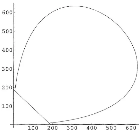
The stopping rule depends on a parameter K which is restricted to integer values, for simplicity. The two stage procedure, NI/(Ch' K), depending on the parameters Ch and K, is defined by: the sample size for the first stage is K and the sample size for the second stage is

{a

_r

c~(s

+

a)(J +

b)l-

K}

where s = SK is the number of observed successes during the first stage and

f

-K - SK is the number of observed failures during the first stage. When the second stage sample size is 0, the sampling terminates after the first stage. The parameters

Ch and K will be determined numerically as described in Section 4.4.

Remark 7. It was suggested by the asymptotic theory that for the fully sequential

procedures only the parameter K needs to be selected and Ch can be taken to be c.

For the two-stage procedure both parameters Ch and K need to be selected

numeri-cally. Our numerical investigation shows that if we restrict Ch to C in the two-stage

procedure, the performance suffers. This was also suggested by the asymptotic theory.

4.3

Lorden's Push Algorithm

In this section we will discuss Lorden's method for constructing confidence intervals

that improve upon the performance of

[Xn -

h,

Xn

+

h]. Lorden shows ([12]) that

in the fixed sample size case one can improve the minimum coverage probability

obtained by fixed width

d

confidence intervals by letting

[L

,

R]

increase as a function

of

Xn

as rapidly as possible, i.e., the intervals [L, R] are pushed to the right as much

as possible. This push algorithm can also be applied in the sequential setting for

any given stopping rule, N (see Theorem 7), and the algorithm constructs the

so-called pushed confidence intervals. The pushed confidence intervals applied to the

stopping rules N* (e, l), N' (K) and Nil (Ch' K) described in the previous sections form the confidence interval procedures that we propose for use.

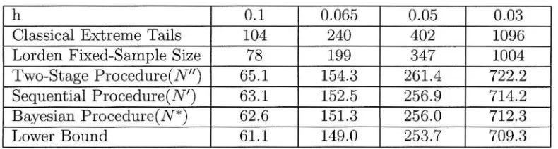
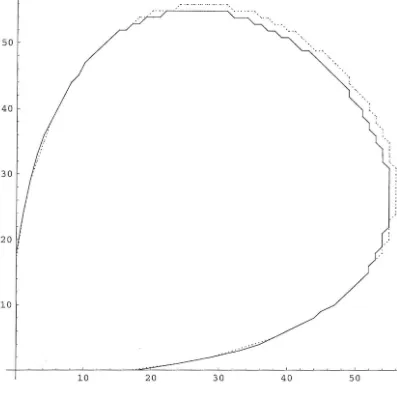
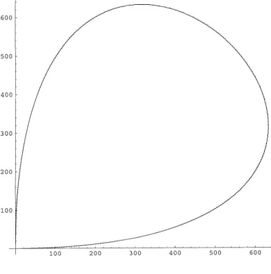
an ordering of the stopping points

(s, 1)

= (S

N,

N - S

N)'

The push algorithm uses

this ordering to set confidence intervals covering smaller p values for smaller points,

i.e., if

(s,

1)

precedes

(s', II)

then

L(s

,

1)

~

L(s',1')

and

R(s

,

i)

~

R(s', I').

In the fixed sample size case the optimal (see [12]) ordering of the stopping points is defined by their maximum likelihood estimate of p, i.e., by the number of successes. In the sequential case such an optimality property is not known, i.e., there is no reasonable conjecture that determines the optimal ordering of the stopping points. In the hope

of achieving near-optimality, we propose to use the maximum likelihood estimate of p, i.e., if

(8,1)

and

(8',1')

are two stopping points, we say that

(8,1)

precedes

(8',1')

if

8/

(s

+

i)

<

s'

/

(s'

+

i')· If

s

/

(s

+

1)

=

s'

/

(s'

+

1')

,

we say that

(8, 1)

precedes

(s', 1')

if s

<

s'. Index the stopping points as

(Si' Ii)

for i = 1, ... ,]. Let J be the index of the

actual stopping point (S N , N - S N ). Now we have to define the confidence interval

[L

,

RJ

for all the possible values of

J,

1, ... ,], so that Land

R

increase as a function of J as rapidly as possible.

There is another consideration that plays an important role. The sample space

of J is finite, and if the confidence intervals are based only on J, then the coverage probability as a function of p will have relatively large jumps at the endpoints of the confidence intervals. Greater efficiency, i.e., larger 1', is achievable by reducing the

size of the jumps through a technique called randomization. Let U be a uniformly distributed random variable on the interval [-0.5,0.5]' independent of the XIs. Let

The optimality property that determines the construction of Lorden's pushed intervals, even in the fixed sample size case, requires that the endpoints Land R of the confidence intervals be restricted to a finite grid {O,

!,

~,

.

.

.

,

rn~l, 1} in order to make a numerical algorithm possible. As explained in [12], the construction of optimal

[L

,

R]

that are not limited to a grid requires taking monotonic majorants, which are not computable. In our numerical investigations we use m = 105_{, so that}

little is lost by this restriction. Theorem 8 shows that ~ is an upper bound on the difference between the unrestricted shortest-width intervals and shortest-width intervals that are grid limited, i.e., that have end points in {O,

!,

...

,

1}. Let Pk

=

!

for k = 0, ... ,m.

Definition 1. A confidence interval

[

L

,

R]

has grid coverage level '"Y if for

k =

1, ... , m

( 4.3)

for P = Pk-l and P = Pk·

Choose m and r so that .I.... _rn = d.

Theorem 6 (Lorden). Grid-limited level '"Y confidence intervals have grid coverage

level '"Y.

Proof. Let

[

L

,

R]

be a grid-limited level '"Y confidence interval. Let Yk =