Expanding Thurston Maps

(1)

arXiv:1009.3647v3 [math.DS] 10 Oct 2017

Expanding Thurston Maps

Mario Bonk

Daniel Meyer

Department of Mathematics, University of California, Los Ange-les, CA 90095, USA

Department of Mathematical Sciences, University of Liverpool Mathematical Sciences Building, Liverpool L69 7ZL, United Kingdom

(2)

2010Mathematics Subject Classification. 37-02, 37F10, 37F20, 30D05, 30L10.

Key words and phrases. Expanding Thurston map, postcritically-finite rational map, visual metric, invariant curve, Markov partition, Latt`es map, subdivision

(3)

List of Figures

1.1 The Latt`es mapg. 3

1.2 The maph. 8

1.3 Polyhedral surfaces obtained from the replacement rule. 9

2.1 The mapg. 37

2.2 An obstructed map. 47

3.1 Invariant tiling for type (244). 55

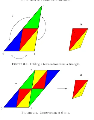
3.4 Folding a tetrahedron from a triangle. 81

3.5 Construction of Θ =℘. 81

3.6 A Lattès map with orbifold signature (2,4,4). 84 3.7 A Lattès map with orbifold signature (3,3,3). 85 3.8 A Lattès map with orbifold signature (2,3,6). 85

3.9 A Euclidean model for a flexible Latt`es map. 87

3.10 The mapf in Example 3.27. 88

4.1 The generator of the snowsphere_S. 99

4.2 The setZ. 101

5.1 The cycle of a vertexv. 110

5.2 A chain, ann-chain, and an e-chain. 123

6.1 A map with a Levy cycle. 151

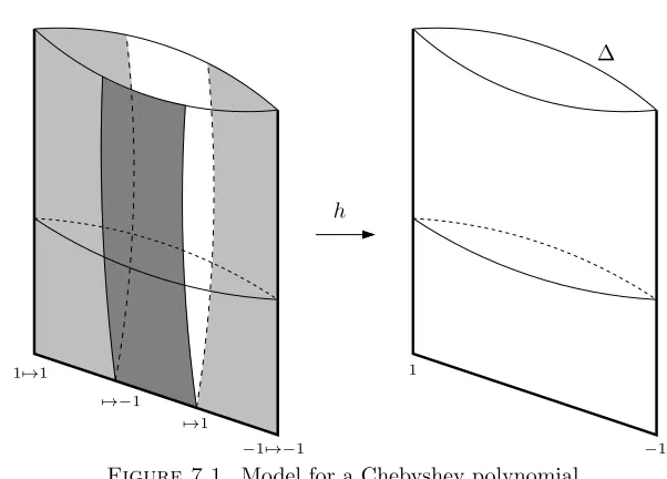
7.1 Model for a Chebyshev polynomial. 166

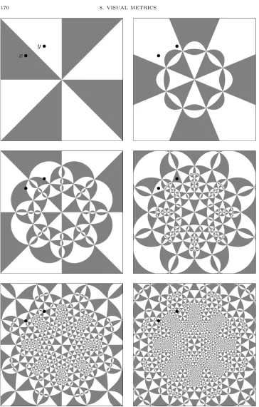
8.1 Separating points by tiles. 170

11.1 Tower of isotopies. 203

11.2 J is not isotopic toS1 _rel._{_1,i_,₋_1,₋i_}_. ₂₀₆

11.3 Constructing a path througha, b, p. 210

11.4 Construction of the curveC′_. ₂₁₄

12.1 Subdividing tiles. 223

(8)

12.2 The proof of Lemma 12.8. 226

12.3 Two subdivision rules. 230

12.4 The two-tile subdivision rule forz2₋_1. ₂₄₁

12.5 Tiles of level 7 for Example 12.20. 242

12.6 The barycentric subdivision rule. 243

12.7 Tiles of levels 1–6 for the barycentric subdivision mapf2. 244

12.8 The 2-by-3 subdivision rule. 245

12.9 Adding flaps. 247

12.10 Two-tile subdivision rule realized byg7. 248

14.1 Equivalence classes of vertex-, edge-, and tile-type. 272 14.2 A two-tile subdivision rule realized by a mapg with post(g)6=V0. 283 14.3 The map f is not combinatorially expanding, but equivalent to the

expanding mapg. 284

15.1 The invariant curve for Example 15.6. 290

15.2 Invariant curves for the Latt`es mapg. 293

15.3 No invariant Jordan curve_{C ⊃}e post(f). 295

15.4 Iterative construction of an invariant curve. 301

15.5 Iterative construction by replacing edges. 306

15.6 Example where_Ceis not a Jordan curve. 308

15.7 A non-trivial rectifiable invariant Jordan curve. 308

16.1 Replacingk-tiles with (k₋1)-tiles. 320

17.1 Bijection of tiles. 340

18.1 Construction ofγ. 348

20.1 The setup in Lemma 20.12. 395

20.2 Connecting tiles by shorte-chains. 399

(9)

Preface

This book is the result of an intended research paper that grew out of control. A preprint containing a substantial part of our investigations was already published on arXiv in 2010. To make its content more accessible, we decided to include some additional material. These additions more than doubled the size of this work as compared with the 2010 version and caused a long delay in its completion.

More than fifteen years ago we became both interested in some basic problems on quasisymmetric parametrization of 2-spheres. This is related to the dynamics of rational maps—an observation we believe was first made by Rick Kenyon. During our time at the University of Michigan we decided to join forces and to investigate this connection systematically.

We realized that for the relevant rational maps an explicit analytic expression is not so important, but rather a geometric-combinatorial description. As this became our preferred way of looking at these objects, it was a natural step to consider a more general class of maps that are not necessarily holomorphic. The relevant properties can be condensed into the notion of anexpanding Thurston mapwhich is the topic of this book. We will discuss the underlying ideas more thoroughly in the introduction (Chapter 1).

Part of this work overlaps with studies by other researchers, notably Ha¨ıssinsky-Pilgrim [HP09], and Cannon-Floyd-Parry [CFP07]. We would like to clarify some of the interrelations of our investigations with these works. Theorem 15.1 (in the body of the text) was announced by the first author during an Invited Address at the AMS Meeting at Athens, Ohio, in March 2004, where he gave a short outline of the proof. After the talk he was informed by Bill Floyd and Walter Parry that related results had been independently obtained by Cannon-Floyd-Parry (which later appeared as [CFP07]).

Theorem 18.1 (ii) was previously published by Ha¨ıssinsky-Pilgrim as part of a more general statement [HP09, Theorem 4.2.11]. Special cases go back to work by the second author [Me02] and unpublished joint work by Bruce Kleiner and the first author. The current, more general version emerged after a visit of the first author at the University of Indiana at Bloomington in February 2003.

During this visit the first author explained to Kevin Pilgrim concepts of quasi-conformal geometry and his joint work with Bruce Kleiner on Cannon’s conjecture in geometric group theory. Kevin Pilgrim in turn pointed out Theorem 11.1 and the ideas for its proof to the first author. After this visit versions of Theorem 18.1 (ii) with an outline for the proof were found independently by Kevin Pilgrim and the first author. A proof of Theorem 18.1 (ii) was discovered soon afterwards by the authors using ideas from [Me02] (see [Me10] for an argument along similar lines) in combination with Theorem 15.1.

(10)

We are indebted to many people. Conversations with Bruce Kleiner, Peter Ha¨ıssinsky, and Kevin Pilgrim have been especially fruitful. We would also like to thank Jim Cannon, Bill Floyd, Lukas Geyer, Misha Hlushchanka, Zhiqiang Li, Dimitrios Ntalampekos, Walter Parry, Juan Souto, Dennis Sullivan, and Mike Zieve for various useful comments. Two anonymous referees provided us with valuable feedback. Their considerable efforts were very much appreciated.

Qian Yin was so kind to let us incorporate parts of her thesis. We are grateful to Jana Kleineberg for her careful proofreading and her help with some of the pictures. We are also happy to acknowledge the patient support of our editors from the American Mathematical Society, Ed Dunne and Ina Mette.

Over the years we received funding from various sources. Mario Bonk was partially supported by NSF grants DMS 0244421, DMS 0456940, DMS 0652915, DMS 1058283, DMS 1058772, DMS 1162471, and DMS 1506099. Daniel Meyer was partially supported by an NSF postdoctoral fellowship, the Deutsche Forschungs-gemeinschaft (DFG-ME 4188/1-1), the Academy of Finland, projects SA-134757 and SA-118634, and the Centre of Excellence in Analysis and Dynamics Research, project No. 271983.

(11)

Notation

We summarize some of the most important notation used in this book for easy reference.

When an object A is defined to be another object B, we write A := B for emphasis.

We denote byN=_{1,2, . . ._}the set of natural numbers and byN0={0,1,2, . . .}

the set of natural numbers including 0. We writeZfor the set of integers, andQ,

R, Cfor the set of rational, real, and complex numbers, respectively. For k ∈N, we letZk=Z/kZbe the cyclic group of orderk.

We also considerNb :=N_{∪ {∞}}. Givena, b∈Nb we writea|bifadividesb. This notation is extended toNb-valued functions. IfA_⊂Nb, then lcm(A)_∈Nb denotes the least common multiple of the numbers inA. See Section 2.5 for more details.

Thefloor of a real numberx, denoted by_⌊x_⌋, is the largest integerm_∈Zwith m _≤x. The ceiling of a real number x, denoted by _⌈x_⌉, is the smallest integer m_∈Zwithx_≤m.

The symbol i _{stands for the imaginary unit in the complex plane} _C_{. The}

real and imaginary part of a complex numberz are indicated by Re(z) and Im(z), respectively, and its complex conjugate byz. The open unit disk inCis denoted by

D:=_{z_∈C:_|z_|<1_}, and the open upper half-plane byH:=_{z_∈C: Im(z)>0_}. We letCb :=C_{∪ {∞}}be the Riemann sphere. It carries the chordal metric σ given by formula (A.5) (in the appendix). Similarly, we letRb :=R_{∪ {∞}}. Here we considerRb as a subset ofCb, and soRb _⊂Cb.

TheLebesgue measure onR2_,_C_,_C_b_{, or}_D_{is denoted by}_L_{. If necessary, we add}

a subscript here to avoid ambiguities. More precisely,L=LR2 andL=L_Care the

Euclidean area measures onR2 _and_C_,

L=LbCis the spherical area measure onCb, andL=LDthe hyperbolic area measure onDconsidered as the hyperbolic plane. When we consider two objects Aand B, and there is a natural identification between them that is clear from the context, we writeA∼=B. For example,R2_∼₌_C

if we identify a point (x, y)_∈R2 _with_x₊_y_i ∈C.

The derivative of a holomorphic functionf is denoted byf′_{as usual. If Ω}

⊂Cb

is an open set andf: Ω_→Cb is a holomorphic map, thenf♯_{stands for its}_spherical derivative (see (A.6)). For a differentiable (not necessarily holomorphic) map, we useDf to denote its derivative considered as a linear map between suitable tangent spaces. If these tangent spaces are equipped with norms, then we let_kDf_k be the operator norm ofDf. Sometimes we use subscripts here to indicate the norms.

Two non-negative quantities a and b are said to be comparable if there is a constantC≥1 (possibly depending on some ambient parameters) such that

1

Ca≤b≤Ca.

(12)

We then write a≍b. The constant C is referred to asC(≍). Similarly, we write a .b or b & a, if there is a constant C > 0 such that a≤ Cb, and refer to the constantC asC(.) orC(&). If we want to emphasize the parametersα,β, . . . on whichCdepends, then we write C(≍) =C(α, β, . . .) etc.

The cardinality of a setX is denoted by #X and the identity map on X by idX. Ifxn ∈X forn∈Nare points inX, we denote the sequence of these points

by_{xn}n∈N, or just by{xn} if the index setNis understood.

Iff: X_→X is a map andn_∈N, then

fn:=f ◦ · · · ◦f

| {z } nfactors

is the n-th iterate of f. We set f0 _{:= id}

X for convenience, but unless otherwise

indicated it is understood thatn_∈Nif we speak of an iterate fn _of_f_.

Letf:X _→Y be a map between sets X and Y. IfU _⊂X, thenf_|U stands for therestriction off to U. IfA⊂Y, thenf−1_{(A) :=}_{_x_∈_X _:_f_(x)_∈_A_} _{is the}

preimage ofA in X. Similarly,f−1_{(y) :=}_{_x_∈_X _:_f_{(x) =}_y_} _{is the preimage of a}

pointy∈Y.

If f: X → X is a map, then preimages of a set A ⊂ X or a point p ∈ X under the n-th iterate fn are denoted by f−n(A) := {x ∈ X : fn(x) ∈ A} and f−n(p) :={x∈X :fn(x) =p}, respectively.

Let (X, d) be a metric space, a _∈ X, and r > 0. By Bd(a, r) = {x ∈ X :

d(a, x)< r_}we denote the open and byBd(a, r) ={x∈X :d(a, x)≤r}the closed

ball of radiusrcentered ata. IfA, B_⊂X, we let diamd(A) be the diameter,Abe

the closure ofAinX, and

distd(A, B) := inf{d(x, y) :x∈A, y∈B}

be the distance ofAandB. Ifp_∈X, we let distd(p, A) := distd({p}, A). Forǫ >0,

Nd,ǫ(A) :={x∈X: distd(x, A)< ǫ}

is the open ǫ-neighborhood of A with respect to d. If γ: [0,1] _→ X is a path, we denote by lengthd(γ) the length of γ. Given Q ≥ 0, we denote by H

Q d the

Q-dimensional Hausdorff measure onX with respect to d. We drop the subscript d in our notation forBd(a, r), etc., if the metric dis clear from the context. For

the Euclidean metric onCwe sometimes use the subscriptCfor emphasis. So, for example,

BC(a, r) :=_{z_∈C:_|z₋a_|< r_} denotes the Euclidean ball of radiusr >0 centered ata_∈C.

TheGromov productof two pointsx, y_∈X with respect to a basepointp_∈Xin a metric spaceX is denoted by (x_·y)por by (x·y) if the basepointpis understood

(see Section 4.2). The boundary at infinity of a Gromov hyperbolic space X is represented by ∂∞X. If a group Gacts on a space X, then we write G yX to

indicate this action.

Often we use the notationI = [0,1]. IfX andY are topological spaces, then ahomotopy is a continuous mapH:X×I→Y. Fort∈I, we letHt(·) :=H(·, t)

be thetime-t mapof the homotopy.

The symbol S2 _{indicates a 2-sphere, which we think of as a topological}

ob-ject. Similarly,T2 _{is a topological 2-torus. For a 2-torus with a Riemann surface}

(13)

NOTATION xiii

Often S2 _{(or the Riemann sphere} _C_b_{) is equipped with certain metrics that}

induce its topology. Thevisual metricinduced by an expanding Thurston mapf is usually denoted by ̺(see Chapter 8). Thecanonical orbifold metric of a rational Thurston map f is indicated byωf (see Section A.10).

The (topological) degree of a branched covering map f between surfaces is denoted by deg(f) and the local degree of f at a point xby deg_f(x) or deg(f, x) (see Section 2.1). We write crit(f) for the set of critical points of a branched covering map (see Section 2.1), and post(f) for the set ofpostcritical points of a Thurston map f (see Section 2.2).

Theramification function of a Thurston mapf is denoted byαf (see

Defini-tion 2.7), and the orbifold associated withf byOf (see Definition 2.10).

For a given Thurston mapf:S2→S2we usually use the symbolC to indicate a Jordan curve_{C ⊂}S2 _{that satisfies post(f}₎

⊂ C.

When we consider objects that are defined in terms of the n-th iterate of a given Thurston map, then we often use the upper index “n” to emphasize this.

For a topological cellc in a topological space_X we denote by∂ctheboundary

ofc, and by int(c) theinterior ofc(see Section 5.1). Note that∂cand int(c) usually do not agree with the boundary or interior ofcas a subset of_X.

Cell decompositions of a space _X are usually denoted by_D (see Chapter 5). Letn_∈N0, f: S2→S2 be a Thurston map, and C ⊂S2 be a Jordan curve with

post(f)_{⊂ C}. We then write_Dn_(f,

C) for the cell decomposition ofS2_{consisting of}

thecells of level norn-cellsdefined in terms off and_C(see Definition 5.14). The set of corresponding n-tiles is denoted byXn_{, the set of} _n_-edges _by _En_{, and the}

set ofn-vertices byVn _{(see Section 5.3).}

In this context we often “color” tiles “black” or “white”. We then use the subscriptsbandwto indicate the color (see the end of Section 5.3). For example, the black and white 0-tiles are denoted byXb0 andXw0, respectively.

The n-flower of an n-vertex v is denoted by Wn(v) (see Section 5.6). The number Dn =Dn(f,C) is the minimal number of n-tiles required to join opposite

sides (see (5.15)).

The numberm(x, y) = mf,C(x, y) is defined in Definition 8.1. The expansion

factor of a visual metric is usually denoted by Λ (see Definition 8.2).

We write Λ0(f) for the combinatorial expansion factor of a Thurston map f

(see Proposition 16.1).

The topological entropy of a map f is denoted by htop(f), and the measure-theoretic entropy off with respect to a measureµbyhµ(f). Themeasure of max-imal entropy of an expanding Thurston mapf is indicated byνf. See Chapter 17

for these concepts.

For a rational Thurston mapf:Cb _→Cb we write Ωf for its canonical orbifold measure(see Section A.10) and, iff is also expanding,λf for the unique probability

(14)

(15)

CHAPTER 1

Introduction

In this work we study the dynamics of Thurston maps under iteration. A Thurs-ton map is a branched covering map on a 2-sphereS2_{such that each of its critical}

points has a finite orbit. The most important examples are given by postcritically-finite rational maps on the Riemann sphereCb. Most of the time we will also assume that a Thurston map is expanding in a suitable sense. For postcritically-finite ra-tional mapsf: Cb _→Cb expansion is equivalent to the requirement thatf does not have periodic critical points or that its Julia set is equal toCb.

These objects were first considered by Thurston as topological model maps in the context of his celebrated characterization of rational maps (see Theorem 2.18). The terminology was introduced by Douady and Hubbard in their proof of this theorem.

Every expanding Thurston map f:S2 _→ _S2 _{gives rise to a type of fractal}

geometry on the underlying sphereS2_{. This geometry is represented by a class of} visual metrics ̺that are associated with the map. Many dynamical properties of the map are encoded in the geometry of the correspondingvisual sphere, meaning S2 _{equipped with a visual metric}_̺.

For example, we will see that an expanding Thurston map is topologically conjugate to a rational map if and only if (S2_{, ̺) is quasisymmetrically equivalent to} b

C(see Section 4.1 for the terminology). For us this relation between dynamics and fractal geometry is one of the main motivations for studying expanding Thurston maps.

In order to define a visual metric for a given Thurston mapf: S2

→S2_{, we will}

extract some combinatorial data fromf. For this we consider a cell decomposition of S2 _{and its pull-backs by the iterates} _fn_{. When} _f _{is expanding, the diameters}

of the cells in these decompositions shrink to 0; so we get discrete approximations of S2 _{that get finer with larger level} _{n. Given two distinct points in} _S2_{, one can}

ask at which level the cell decompositions will allow us to distinguish them. Our definition of a visual metric is based on this information.

The visual sphere (S2, ̺) of an expanding Thurston map is fractal in the sense that its Hausdorff dimension is typically larger than 2. With a suitable choice of ̺, the local behavior off becomes very simple though. Namely, there is a number Λ>1 (theexpansion factor of̺) such thatf expands̺locally by the factor Λ in a sense that will be made precise. So the local behavior off on (S2_{, ̺) is simplified}

at the expense of a more complicated geometry of (S2_{, ̺). This point of view is in}

contrast to the usual setting for complex dynamics, where one studies the action of a rational map on a smooth underlying space, namely the Riemann sphere Cb, considered as a Riemann surface.

(16)

It is possible to construct a graphG that combines the combinatorial data of the cell decompositions on all levels generated by an expanding Thurston map and its iterates. This graphG is Gromov hyperbolic and its boundary at infinity can naturally be identified with the underlying sphere S2_{. Under this identification a}

metric is a visual metric for the given mapf according to our definition if and only if it is a visual metric in the sense of Gromov hyperbolic spaces. This fact relates the study of expanding Thurston maps and of Gromov hyperbolic spaces.

There is an intriguing connection of these ideas toCannon’s conjecturein geo-metric group theory. Roughly speaking, this conjecture predicts that a groupGthat shares the topological properties of the fundamental group of a closed hyperbolic 3-manifold “is” such a fundamental group (see Section 4.3 for precise statements). In this context one assumes that the groupG is Gromov hyperbolic and that its boundary at infinity ∂∞G is a 2-sphere. Here ∂∞Gis naturally equipped with a

visual metric that provides∂∞G with a fractal geometry. Then Cannon’s

conjec-ture is equivalent to showing that the fractal sphere ∂∞G is quasisymmetrically

equivalent toCb.

So for both types of dynamical systems, namely expanding Thurston maps and Gromov hyperbolic groupsGwith 2-sphere boundary∂∞G, we are led to the

investigation of a fractal geometry on the underlying 2-sphere. This analogy can be viewed as an example ofSullivan’s dictionarywhich exhibits similarities in complex dynamics and the theory of Kleinian groups. Common to both areas is the desire to characterize conformal dynamical systems in a wider class of dynamical systems characterized by suitable metric-topological conditions. One should not push the analogies too far though: while Cannon’s conjecture is generally believed to be true and, accordingly, one expects that the fractal 2-spheres arising from Gromov hyperbolic groups are always quasisymmetrically equivalent toCb, this is not always the case for Thurston maps, because not every Thurston map is equivalent to a rational map.

After these remarks about some of the motivations for our investigation, we now state some basic definitions more precisely (more details can be found in Chapter 2). Letf:S2

→S2 _{be an (orientation-preserving) branched covering map. As usual,}

we call a point c _∈ S2 _a _{critical point} _of _f _{if near} _c _{the map} _f _{is not a local}

homeomorphism. Apostcritical pointis any point obtained as an image of a critical point under forward iteration of f. So if we denote by crit(f) the set of critical points off and byfn _the_{n-th iterate of}_f_{, then the set of postcritical points of}_f

is given by

post(f) := [

n≥1

{fn(c) :c_∈crit(f)_}.

It is a fundamental fact in complex dynamics that much information on the dynamics can be deduced from the structure of the orbits of critical points. A very strong assumption in this respect is that each such orbit is finite, i.e., that post(f) is a finite set. In this case the map f is called postcritically-finite. A

Thurston map is a (non-homeomorphic) branched covering mapf: S2

→S2 _that

is postcritically-finite.

Thurston maps are abundant and include specificrational Thurston maps(i.e., rational maps onCb that are postcritically-finite) such asf(z) = 1−2/z2_or_f_{(z) =}

1 + (i₋_1)/z4_{. More examples can be found in Section 12.3, and a list of examples}

(17)

1.1. A LATT`ES MAP AS A FIRST EXAMPLE 3

0

1

−1

∞

17→0

7→1 07→0

7→−1

−17→0

7→1

∞7→0

7→−1 g

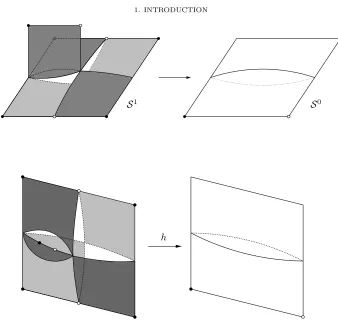
7→∞

Figure 1.1. The Latt`es mapg.

method for producing Thurston maps (see Proposition 12.3); it follows from one of our main results (Theorem 15.1) that at least some iterate of every expanding Thurston map can be obtained from this construction.

We now turn to the discussion of more specific topics in this introductory chapter. Our main purpose is to give some guidance for the intuition of the reader. We will present some examples and discuss the main concepts and results of this work. Full details can be found in subsequent chapters.

1.1. A Latt`es map as a first example

Latt`es maps form a large class of well-understood Thurston maps. They are rational maps obtained as quotients of holomorphic torus endomorphisms. They were the first known examples of rational maps whose Julia set is the whole sphere. We will discuss these maps in more detail in Chapter 3; results concerning them will be outlined in Section 1.7. Note that the terminology is not uniform and some authors use the term Latt`es map with a slightly different meaning.

We will encounter Latt`es maps quite often in this book. On the one hand, they are easy to visualize and construct, and thus often serve as convenient examples to illustrate various phenomena. On the other hand, these maps are quite special and arise in many situations as exceptional cases. In order to introduce some of the main themes of this work, we will now consider a specific Latt`es map.

The map is essentially given by Figure 1.1. We will explain this picture in detail momentarily, but we will first define the map by a more standard approach. This may be helpful for readers that are already familiar with Latt`es maps.

The square [0,1₂]2 _⊂_R2 ∼₌ _C _{can be mapped conformally to the upper}

half-plane in Cb such that the vertices 0,1₂,1₂ + i

2,

i

2 of the square are mapped to the

points 0,1,∞,−1, respectively. Note that here and in the following a “conformal map” is always bijective. By Schwarz reflection we can extend this to a holomorphic map Θ :C_→Cb. Up to postcomposition with a M¨obius transformation, this map is a classicalWeierstraß ℘-function; it is doubly-periodic with respect to the lattice Γ :=Z_⊕Zi _{and induces a double branched covering map of the torus}_T_:=_C_{/Γ to}

(18)

Consider the map

A: C_→C, u_7→A(u) := 2u.

From the properties of the ℘-function or directly from the definition of Θ by the reflection process, one can see that Θ(v) = Θ(u) foru, v∈Cif and only ifv=±u+γ withγ∈Γ. In this case, Θ(2v) = Θ(2u). This implies that there is a well-defined and unique holomorphic mapg:Cb _→Cb such that the diagram

(1.1) C A //

Θ

C

Θ

b

C g //Cb

commutes. The mapg obtained in this way is aLatt`es map. It is a rational map. One can show that it is given by

g(z) = 4z(1−z

2₎

(1 +z2₎2 forz∈Cb,

and that the Julia set ofg is the whole sphere.

More relevant for us than this explicit formula for g is that one can describe g geometrically as indicated in Figure 1.1. To explain this, note that there is an essentially unique path metric onCb obtained as a “push-forward” of the Euclidean metric onCby the map Θ. This metric is in fact thecanonical orbifold metric of g (see Section A.10 and Section 2.5).

Geometrically, the sphere equipped with this metric looks like a pillow. In general, apillow (see Section A.10) is a metric space P obtained from gluing two identical copies Xw and Xb of a (simple and compact) Euclidean polygonX ⊂C

together along their boundaries. The pillow is equipped with the induced path metric. Under the given identification, ∂Xw∼=∂Xbis a Jordan curve in the pillow

P called itsequator.

In our case, the upper and lower half-planes inCb equipped with the canonical orbifold metric are isometric to copies of the squareS = [0,1/2]2_{. If we glue two}

copies ofS together along their boundaries, then we obtain the pillowP. We color one of these squares, say the one corresponding to the upper half-plane, white, and the other square black.

The squareS = [0,1/2]2

⊂R2 _∼₌_C _{(and each of its translates by} 1

2(m+ni)

wherem, n_∈Z) can be subdivided into four squares of side length 1/4. IfS′_{is such}

a square, then A(S′_{) is a square of side length 1/2 that is mapped by Θ to either}

the upper or the lower half-plane, meaning to either the black or the white face of the pillowP. It follows from (1.1) thatg has a very similar mapping behavior on P.

(19)

1.1. A LATT`ES MAP AS A FIRST EXAMPLE 5

The vertices where four small squares intersect are the critical points ofg. They are mapped bygto the set{1,∞,−1}, which in turn is mapped to {0}. The point 0 is a fixed point ofg. Sogis a postcritically-finite branched covering map on the 2-sphereP with post(g) ={0,1,∞,−1}, and hence a Thurston map. The postcritical points ofg are the vertices of the pillow, which are the conical singularities of our canonical orbifold metric. The extended real lineC:=Rb =R_∪{∞}(corresponding to the equator of the pillow) is a Jordan curve that is invariant undergin the sense that g(C)⊂ C and contains the set {0,1,∞,−1} of postcritical points of g. The set g−1₍

C) is an embedded graph in the pillow consisting of all sides of the small squares on the left hand side of Figure 1.1 as edges and the points ing−1_(post(g)),

i.e., the corners of these squares, as vertices. This graph g−1₍

C) determines the tiling in this picture.

The set g−2₍

C) is obtained by pulling g−1₍

C) back by the map g. Since g restricted to any small square S′ _{is a homeomorphism onto one of the two large}

squaresS forming the pillow, in this processS′ _{is subdivided in the same way as}_S

was subdivided by the small squares of side length 1/4 (i.e., S′ _{is subdivided into}

4 squares). It follows that g−2₍_C_{) subdivides the pillow into 4}_×_{8 = 32 squares}

of side length 1/8. Proceeding in this way inductively, we see that the preimage g−n₍_C_{) of}_C _{under the iterate} _gn _{subdivides the pillow into 2}_·₄n _{squares of side}

length 2−n−1 _for_n_∈_N_.

The complementary components ofg−n₍_C_{) are the interiors of these squares. In}

particular, the diameters of these components tend to 0 uniformly asn_{→ ∞}. This fact will be the basis of our definition of anexpanding Thurston map. Accordingly, g is such a map.

For each n _∈ N the set g−n₍

C) forms an embedded graph in the pillow P with the points in g−n_{(post(g)) as vertices. This is also meaningful for} _n_{= 0, if}

we interpretg0 _{as the identity map on the pillow}_P_{. Then this graph is just the}

Jordan curve_C with the points in post(g) as vertices. The graphg−n₍

C) is the 1-dimensional skeleton or 1-skeleton of acell decom-position _Dn ₌

Dn_(g,

C) of the pillowP generated by g and _C (see Chapter 5 for the terminology that we use here and below). The 2-dimensional cells or tiles of the cell decomposition_Dn _{are squares of side length 2}−n−1 _{and are given by the}

closures of the complementary components ofg−n₍_C_{) in}_P_{. The map}_g_{sends each}

cell inDn+1 _{homeomorphically to a cell in}_Dn _{(for all}_n_∈_N

0); sog iscellular for

each pair (Dn+1_,_Dn_{) of cell decompositions.}

Since_Cisg-invariant in the sense thatg(_C)_{⊂ C}, we haveg−n₍

C)_⊂g−(n+1)₍ C) for eachn _∈ N0. This inclusion for 1-skeleta implies that the cell decomposition Dn+1 _{is a} _refinement_of

Dn_{. On a more intuitive level, this means that the tiles in} Dn _{are subdivided by the tiles in}

Dn+1_.

The tiles in_D0_{are the two initial squares of side length 1/2 forming the pillow,}

and _D1 _{is formed by squares of side length 1/4 subdividing these squares. Since}

we repeat the same subdivision procedure in the passage from Dn _to _Dn+1_{, this}

whole sequence of cell decompositionsDn _{is essentially generated by the initial pair}

(D1_,

D0_{). This pair (} D1_,

D0_{) is a}_{cellular Markov partition}_for_g_{(see Definition 5.8).}

The map g sends each cell in D1 _{to a cell in}

D0_{. The cellular Markov partition}

(D1_,

D0_{) together with this information completely determines the map} _g _{(up to}

(20)

In fact, one can turn this process around and construct g from this combina-torial data, meaning essentially from the information encoded in Figure 1.1. A related discussion can be found in Section 1.5.

1.2. Cell decompositions

The previous example motivates several concepts for a general Thurston map f:S2

→S2_{, in particular the combinatorial description of}_f _{that we will employ.}

We choose a Jordan curve_{C ⊂} S2 _{with post(f}₎

⊂ C, and consider the preim-agesf−n₍

C). Then for eachn _∈N0 one obtains an associated cell decomposition Dn₌

Dn_(f,

C) ofS2_{. Its vertices are the points in}_f−n_(post(f_{)), and its 1-skeleton}

the setf−n₍

C). The condition post(f)_{⊂ C} ensures that the closure of each com-plementary component of f−n₍

C) is a closed Jordan region. These sets are the 2-dimensional cells in_Dn_{. We call each such set a}_{tile of level}_n_{or an}_n-_tile_{(of the}

cell decomposition). Similarly, we call any pointv_∈f−n_(post(f_{)) a}_vertex _{of level}

nor ann-vertex; then{v} is a 0-dimensional cell inDn_{. Finally, the closure}_e_{of a}

component off−n₍_C₎_\_f−n_(post(f_{)) is called an}_edge _{of level}_n_{or an}_n_-edge_{; then}

e is a 1-dimensional cell ofDn_{. The cells in} _Dn_(f,_C_{) of any dimension are called}

then-cellsfor givenf andC. Note that herenalways refers to the level of the cell and not to its dimension.

The cell decompositionD0_{contains two tiles (the two closed Jordan regions in}

S2 bounded byC), k = # post(f) vertices (the points p ∈post(f)), and k edges (the closed arcs into which the points in post(f) divide C). We will study cell decompositions and their relation to Thurston maps in more detail in Chapter 5. Various examples for the cell decompositions_Dn_{generated in this way can be found}

in Figures 8.1, 12.1, 12.7, and 15.1. We say that a Thurston mapf:S2

→S2_is_expanding_{if there exists a Jordan}

curve_{C ⊂}S2_{with post(f}₎

⊂ Csuch that the complementary components off−n₍ C) become uniformly small in diameter asn_{→ ∞}. HereS2_{is equipped with any metric}

inducing the topology on S2_{. It is easy to see that this condition is independent}

of the choice of this base metric. Later we will show that it is also independent of the choice ofC and will give other characterizations of expansion (see Chapter 6, in particular Proposition 6.4). A rational Thurston map f: Cb _→ Cb is expanding precisely if it does not have periodic critical points or if its Julia set is equal toCb

(see Proposition 2.3). Note that in general a (non-rational) expanding Thurston map may have periodic critical points (see Example 12.21).

Put differently, a Thurston mapf is expanding if and only if the tiles in_Dn₌ Dn_(f,

C) shrink to 0 in diameter uniformly as n_{→ ∞}. This allows us to describe points in S2 _{by suitable sequences of tiles. So we can think of}

Dn _{as a discrete}

approximation ofS2_{that becomes finer with larger}_n.

We have seen that for the example g discussed in the previous section the n-tiles become uniformly small in diameter as n_{→ ∞}; so we conclude thatg is an expanding Thurston map.

Often the precise choice of the Jordan curveC with post(f)⊂ C will play no essential role, meaning that we may chose any such curve for our considerations. If the curveC is not f-invariant, then in general the cell decompositions Dn _will

(21)

1.3. FRACTAL SPHERES 7

is f-invariant. We will discuss existence of such invariant Jordan curves and the resulting combinatorial description of Thurston maps in Section 1.5.

1.3. Fractal spheres

We want to motivate other important concepts of our investigation, in partic-ular the concept of visual metrics. To do this, we will discuss another Thurston map and an associated fractal 2-sphere. As our main purpose here is to provide the reader with some intuition on the definition of a visual metric̺and on the fractal nature of the sphere (S2_{, ̺), we will omit the justification of some details.}

The map arises from a geometric construction that is similar to the one used to describe the Latt`es map in Section 1.1. Again we start with a pillow obtained by gluing together two squares along their boundaries; see the top right of Figure 1.2. This pillow is a polyhedral surface_S0 _{homeomorphic to the 2-sphere. It carries a}

natural cell decomposition D0 _{with the two squares as tiles, the four sides of the}

common boundary of the squares as edges, and the four common corners of the squares as vertices. To distinguish them from other topological cells that we will introduce momentarily, we consider them as cells of level 0 and accordingly call them 0-tiles, 0-edges, and 0-vertices. As in the example of Section 1.1, we assign colors to the tiles; say the top square of_S0 _{as shown in Figure 1.2 is white, and the}

bottom square is black.

To obtain cells on the next level 1, each of the two squares, or more precisely 0-tiles, is divided into four squares of half the side length. We call these eight smaller squares tiles of level 1, or simply 1-tiles. The edges of these squares are 1-edges. We slit the sphere along one such 1-edge in the white 0-tile and glue in two small squares at the slit, as indicated on the upper left in Figure 1.2. This gives two additional 1-tiles and we obtain a polyhedral surface _S1 _{homeomorphic to the}

2-sphere. The surface_S1_{carries a cell decomposition given by the topological cells of}

level 1 as described. We color the 1-tiles black and white in a checkerboard fashion so that 1-tiles sharing an edge have different color, as indicated in Figure 1.2.

To define a Thurston map based on our construction, we choose an identification of the polyhedral surfaceS1 _with _S0_{. To do this, we represent the six 1-tiles that}

replaced the white 0-tile topologically as subsets of this tile, and similarly the other four 1-tiles as subsets of the black 0-tile. So the 0-tiles are “subdivided” by 1-tiles. This is indicated on the lower left in Figure 1.2. Under this identification the cell decomposition of_S1_{gives a cell decomposition}

D1_on

S0 _{that is a refinement of the}

cell decomposition_D0_.

Now we can define a Thurston map as follows. We map each white 1-tile on the polyhedral surface_S1 _{to the white 0-tile in}

S0_{, and each black 1-tile in}

S1 _{to the}

black 0-tile in_S0_{by a similarity map (preserving orientation). This is a well-defined}

and uniquely determined map on_S1_{if we do this so that the 1-vertices marked by}

a black or a white dot on the upper left in Figure 1.2 are sent to 0-vertices in the upper right of the picture with the same markings.

If we identifyS1_with_S0_{as discussed, we get a map}_h_:_S2_→_S2_{on the 2-sphere}

S2 _:=_S0_{. Since} _h_{restricted to each 1-tile is a homeomorphism onto a 0-tile,} _h_is

(22)

S0 S1

[image:22.612.135.473.90.419.2]

h

Figure 1.2. The maph.

Note that the equator_Cof the pillow is anh-invariant Jordan curve (i.e.,h(_C)_{⊂ C}) and that the cell decomposition_D1 _on

S1_∼₌

S0_{is determined by}_h−1₍

C). Namely, h−1₍_C_{) is a topological graph that gives the 1-skeleton of this cell decomposition,}

and each 1-tile is the closure of a complementary component ofh−1₍_C_).

The relevant information on the map h is contained in the combinatorics of the cell decompositions D0 _and _D1 _{and a map} _L: _D1 _{→ D}0 _{that records how}_h

associates the cells in D1 _{with cells in} _D0_{. This triple (}_D1_,_D0_{, L) forms a} two-tile subdivision rulethat is realized by h. We will give precise definitions of these concepts in Chapter 12. The maphdepends on choices and is not uniquely deter-mined, but another map realizing the same subdivision rule (_D1_,

D0_{, L) is}_Thurston equivalenttoh(see Definition 2.4 for the terminology).

There is no rational map that realizes this combinatorial picture as our map h. More precisely,h is not Thurston equivalent to a rational map, becausehhas a Thurston obstruction. This, together with the terminology, will be explained in Section 2.6.

We will now describe a fractal sphereSthat is associated with our construction and gives an alternative way to view our maph. The sphereS is obtained similarly as the well-known snowflake curve. We will also define a metric̺onS.

To construct the spaceS, we do not identify the surfacesS0 _and_S1_{. Instead,}

we consider the passage from S0 _to _S1 _{as a replacement procedure. The white}

(23)

1.3. FRACTAL SPHERES 9

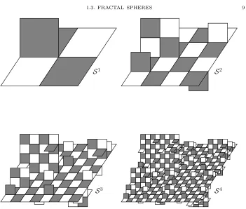
S1

S2

S3

[image:23.612.136.487.89.387.2]

S4

Figure 1.3. Polyhedral surfaces obtained from the replacement rule.

side length 1/2; we call this top part of_S1 _the_{white generator}_{. Similarly, the four}

1-tiles subdividing the black 0-tile form theblack generator. The polyhedral surface

S1 _{consisting of ten squares is the first approximation of the fractal space} S that we are about to construct by iterating this procedure.

Namely, the 1-tiles of the black and white generators are also colored as in-dicated in Figure 1.2. So if we replace each black or white 1-tile with a suitably scaled copy of the black or white generators, then we obtain a polyhedral surface

S2 _{glued together from squares of side length 1/4 as 2-tiles. Here we have to be}

careful about how precisely a tile is replaced with an appropriate generator, because the generators with their given colorings of tiles are not symmetric with respect to rotations. To specify the replacement rule uniquely, we use the additional markings of some points. Each generator carries two points corresponding to the points on

S0 _{marked black or white. In the replacement process we require that these points}

match the corresponding points with the same markings on 1-tiles.

If we iterate the replacement procedure in this way, we obtain polyhedral sur-faces_Sn_{for all levels}_n

∈N0glued together from squares of side length 1/2n. Each

surfaceSn _{carries a natural cell decomposition}_Dn _{given by these squares as tiles.}

Some iterates of this construction are shown in Figure 1.3. The pictures essentially indicate the gluing pattern of the squares which give the surfaces. One should view them as abstract polyhedral surfaces, and not confuse them with the underlying subsets ofR3_{in these pictures. Each surface}_Sn_{is a topological 2-sphere and carries}

(24)

One can now extract a self-similar “fractal” space S as a limit Sn _{→ S} _for

n → ∞ in several ways. One possibility is to pass to a Gromov-Hausdorff limit of the sequence (Sn_{, ̺}

n) of metric spaces. We will discuss a different method that

is closer in spirit to our general definition of a visual metric (see Chapter 8 and Chapter 10; similar considerations appear in Chapter 14).

Namely, given ann-tile _Xn

⊂ Sn _{(which is a square of side length 2}−n_{), and}

an (n+ 1)-tile _Xn+1

⊂ Sn+1_{, we write} Xn _❂

Xn+1 _if

Xn+1 _{is contained in the}

scaled copy of a generator that replaced_Xn _{in the construction of}

Sn+1 _from Sn_.

We now consider descending sequences_X0_❂ X1_❂

X2_❂_{. . .} _{. On an intuitive level}

the squares in such a sequence should shrink to a point in our desired limit space

S represented by the sequence. Here we consider two sequences _{Xn

} and _{Yn }

as equivalent and representing the same point if _Xn ∩ Yn

6

=_∅ for all n_∈ N0. It

is not hard to see that this indeed defines an equivalence relation for descending sequences. By definition our limit space_S is now the set of all equivalence classes.

Forx, y_{∈ S} we set

(1.2) ̺(x, y) := lim sup

n→∞ dist̺n(X

n_, Yn_),

where_{Xn

}and_{Yn

} are sequences representingxandy, respectively. Then̺is well-defined and one can show that this is a metric on_S.

Forx, y_{∈ S},x₆=y, we define

(1.3) m(x, y) := inf{n∈N:Xn

∩ Yn ₌ ∅}, where the infimum is taken over all sequences _{Xn

} and_{Yn

} representingxand y, respectively. Then

(1.4) ̺(x, y)_≍2−m(x,y)

forx, y _{∈ S},x₆=y. This notation (which will be used frequently) means that there is a constantC_≥1 such that

1

C̺(x, y)≤2

−m(x,y)

≤C̺(x, y).

We refer to the constantC asC(≍) in such inequalities. In the present case,C(≍) does not depend on x, y, or n. So roughly speaking, the distance of two distinct points inSis given in terms of the minimal level on which two descending sequences representing the points can distinguish them.

It is intuitively clear that (_S, ̺) is a topological 2-sphere. To outline a rigorous proof for this fact, we return to the Thurston map h defined above. Recall that

C ⊂S2_{is the}_{h-invariant Jordan curve given by the common boundary of the 0-tiles.}

The curve _C contains the vertices of the pillow, which are the postcritical points of h. We consider the cell decompositions _Dn_(h,

C) as discussed in the previous section. Note that the 1-tiles (i.e., the tiles in _D1_(h,

C)) are exactly the 1-tiles in

S1 _{under the identification} S1_∼₌

S0₌_S2_{(see the bottom left in Figure 1.2).}

The maphn _{sends each}_{n-tile to a 0-tile homeomorphically, and we can assign}

colors to n-tiles so that hn _{sends an} _{n-tile to the 0-tile of the same color. In the}

passage fromDn_(h,_C_{) to}_Dn+1_(h,_C_{) each}_{n-tile is subdivided by (n}_{+ 1)-tiles in the}

same way as the 0-tile of the same color is subdivided by 1-tiles. From this it is clear that there is a one-to-one correspondence betweenn-tiles inSn _and_{n-tiles for the}

(25)

1.4. VISUAL METRICS AND THE VISUAL SPHERE 11

we have

Xn+1❂Xn ⇔ Xn+1⊃Xn, and

Xn ∩ Yn

6

=∅ ⇔ Xn∩Yn6=∅,

where then-tilesXn _and _Yn _in _Sn _{and the (n}_{+ 1)-tile}_Xn+1 _in _Sn+1 _correspond

to then-tilesXn _and_Yn _{and the (n}_{+ 1)-tile}_Xn+1 _{for (h,}_C_{), respectively.}

Recall from Section 1.2 thathis expanding if the diameters ofn-tiles for (h,C) tend to 0 uniformly asn→ ∞(with respect to some fixed base metric onS2

rep-resenting the topology). In this case one obtains a well-defined mapϕ:_{S →}S2_by

sending a point in_Srepresented by a descending sequence_{Xn

}to the unique point in the intersectionT_n_∈N0X

n_{of the corresponding}_{n-tiles for (h,}

C). In general, our map hneed not be expanding, but we may assume this if we choose the identifi-cation of_S1 _with

S0 _{carefully (this hinges on the fact that}_h_{is “combinatorially}

expanding” and so the map can be corrected if necessary to make it expanding; see Theorem 14.2 for details). It is then not hard to see thatϕis a homeomorphism, and so_S is a 2-sphere.

Though (_S, ̺) is a topological 2-sphere, it is not aquasisphere. This means that this space is not quasisymmetrically equivalent to the standard 2-sphere (i.e., the unit sphere inR3_{, or equivalently the Riemann sphere}_C_b _{equipped with the chordal}

metric; see Section 4.1 for the definition of a quasisymmetry). This is closely related to the fact thathis not (equivalent to) a rational map. One can deduce that (S, ̺) is not a quasisphere from a general result (see Theorem 18.1 (ii) mentioned in the next section), but one can also show this directly (we will outline an argument in Section 4.4).

The fractal sphere (_S, ̺) is in a sense the natural domain for our maph; namely, we can conjugate our original maph:S2

→S2_{by the homeomorphism}_ϕ:

S →S2

to obtain a map on_S, also denoted byh. We also obtainn-tiles in_S corresponding to then-tiles inS2_{under the homeomorphism}_{ϕ. Roughly speaking, an}_{n-tile in}

S

is the part of_S that “sits on top” of ann-tile in_Sn_{. The new map}_h_:

S → S then behaves locally like a similarity map: it scales each (n+ 1)-tile in_S by a factor 2 and matches it with the correspondingn-tile.

1.4. Visual metrics and the visual sphere

After this example we return to the general setting. Let f: S2

→ S2 _{be an}

expanding Thurston map. We fix a Jordan curve_{C ⊂}S2_{with post(f}₎

⊂S2_{. Then}

forn_∈N0 we have cell decompositionsDn =Dn(f,C) with 1-skeletonf−n(C) as

defined in Section 1.2.

Since f is expanding, the diameters of n-tiles (i.e., tiles in _Dn_{) shrink to 0}

uniformly asn→ ∞. So ifx, y∈S2_{are distinct points and}_Xn _and_Yn_{are tiles of}

leveln withx∈Xn _and _y_∈_Yn_{, then}_Xn_∩_Yn ₌_∅ _{for sufficiently large}_{n. This}

implies that the number

m(x, y) := max_{n_∈N0: there exist non-disjoint n-tiles

(1.5)

Xn _and _Yn _with_x

∈Xn_{, y} ∈Yn

}

(26)

Generalizing (1.4), we consider metrics̺onS2_satisfying

̺(x, y)_≍Λ−m(x,y),

for some Λ>1. We call such a metric a visual metric forf, and Λ its expansion factor. We will start investigating visual metrics in earnest in Chapter 8.

Visual metrics for a given Thurston map f are not unique, but two different visual metrics with the same expansion factor are bi-Lipschitz equivalent. They are snowflake equivalent if they have different expansion factors (see Section 4.1 for this terminology). Whether a metric is visual does not depend on the choice of the Jordan curve_Cthat was used to define the quantity (1.5) via the cell decompositions

Dn_(f,

C). Moreover, if F =fk _{is an iterate of} _f _(where _k

∈N), then a metric is visual forf if and only if it is visual forF. These (and other) basic properties of visual metrics can be found in Proposition 8.3.

Ifσis a tile or an edge in the cell decomposition_Dn ₌ Dn_(f,

C), then diam̺(σ)≍

Λ−n_{. In addition, any two disjoint cells}_{σ, τ}

∈ Dn _{satisfy dist}

̺(σ, τ)&Λ−n. This

notation means that there is a constantC >0 such thatCdist̺(σ, τ)≥Λ−n. We

refer to the constantCasC(&). Equivalently, we write Λ−n_._dist

̺(σ, τ) and refer

to the constantC as C(.). Here the constantsC(_≍) andC(&) do not depend on nor the cells involved. In fact, these two geometric properties characterize visual metrics (see Proposition 8.4).

For the map g from Section 1.1 the length metric induced by the Euclidean metric on the pillowP is a visual metric with expansion factor Λ = 2. Similarly, the particular metric̺defined in Section 1.3 is a visual metric forhwith expansion factor Λ = 2 (here we identifyS withS2 _{by the homeomorphism}_{ϕ). In this case,}

we obtain visual metrics with arbitrary expansion factor 1<Λ_≤2 if we consider a “snowflaked” metric̺α _{with suitable}_α

∈(0,1], but there is no visual metric for hwith Λ>2. Indeed, if̺is a visual metric with expansion factor Λ>1 andXn

is an n-tile, then diam̺(Xn) . Λ−n. Now it is easy to see that one can form a

connected chain ofn-tiles with 2n_{elements that joins two non-adjacent 0-edges (as}

Figure 1.3 suggests, one obtains such a chain by running along the bottom 0-edge). Then by the triangle inequality 2n

·Λ−n_&_{1 for all}_n

∈N, and so Λ_≤2. Let f: S2

→ S2 _{be an expanding Thurston map. Then the supremum of all}

Λ>1 for which there exist visual metrics with expansion factor Λ agrees with the

combinatorial expansion factor of f, denoted by Λ0(f). It is computed from data

associated with the cell decompositionsDn_(f,_C_{) determined by the map}_f _{and a}

Jordan curve C ⊂ S2 _{with post(f}₎ _{⊂ C}_{. For this we consider the combinatorial}

quantity Dn(f,C) defined to be the minimal number of tiles in Dn(f,C) that are

needed to form a connected set joining opposite sides ofC, i.e., two non-adjacent 0-edges (the definition is slightly different in the case # post(f) = 3; see Section 5.7). For the examples discussed in Sections 1.1 and 1.3 we have Dn(g,C) = 2n and

Dn(h,C) = 2n forn∈N0.

In general, the number Dn(f,C) depends on C. For an expanding Thurston

map it grows at an exponential rate asn_{→ ∞}. This growth rate is independent of

C, and determined only byf. Moreover, the limit

(1.6) Λ0(f) := lim

n→∞Dn(f,C)

1/n

exists, satisfies 1<Λ0(f)<∞, and is defined to be the combinatorial expansion

(27)

1.4. VISUAL METRICS AND THE VISUAL SPHERE 13

well-behaved under iteration (see Proposition 16.2). For our two examples we have Λ0(g) = 2 and Λ0(h) = 2.

As already mentioned above, Λ0(f) gives the range of possible expansion factors

of visual metrics for an expanding Thurston map f. This is made precise in the following theorem.

Theorem 16.3(Visual metrics and their expansion factors). Letf:S2 →S2 be an expanding Thurston map, andΛ0(f)∈(1,∞)be its combinatorial expansion factor. Then the following statements are true:

(i) IfΛ is the expansion factor of a visual metric for f, then1<Λ_≤Λ0(f).

(ii) Conversely, if 1 < Λ <Λ0(f), then there exists a visual metric ̺ for f with expansion factor Λ. Moreover, the visual metric ̺ can be chosen to have the following additional property:

For everyx∈S2 _{there exists a neighborhood} _U

x of xsuch that

̺(f(x), f(y)) = Λ̺(x, y)for ally∈Ux.

(Note that in this introduction we label the results as they appear in later chapters.)

In general, one cannot guarantee the existence of a visual metric with expansion factor Λ = Λ0(f) (see Example 16.8).

The combinatorial expansion factor always satisfies the inequality Λ0(f) ≤

deg(f)1/2_{, where deg(f}_{) is the (topological) degree of}_f _{(see Proposition 20.1). For}

our examples g and hfrom the previous sections we have Λ0(g) = 2 = deg(g)1/2

and Λ0(h) = 2 < deg(h)1/2 = √5. The equality for the Latt`es map g is not a

coincidence. Closely related results will be discussed in Section 1.7.

According to Theorem 16.3 (ii), for each expanding Thurston map f we can find a visual metric ̺ so that f scales the metric ̺ by a constant factor at each point. The Latt`es mapg:Cb _→Cb discussed in Section 1.1 illustrates this statement: if we equip Cb with a suitable visual metric forg (the path metric on the pillow in Figure 1.1), then g behaves like a piecewise similarity map, where distances are scaled by the factor Λ = 2.

The spaceS from Section 1.3 equipped with the visual metric̺ in (1.2) is a fractal sphere. It is self-similar in the sense that the part of the surface that is “built on top” of some n-tile Xn _{is similar (i.e., is isometric up to scaling by the}

factor 2n_{) to the part of the surface that is “built on top” of the white or the black}

0-tile. Similarly, we can find visual metrics for any Thurston map f such that f scales tiles by a constant factor. Then the metric behavior of the dynamics on tiles becomes very simple, while the space on whichf acts is a fractal sphere and geometrically more complicated.

Our choice of the term “visual metric” is motivated by the close relation of this concept to the notion of a visual metric on the boundary of a Gromov hyperbolic space (see Section 4.2 for general background; very similar ideas can be found in [HP09]). Namely, if f:S2

→ S2 _{is an expanding Thurston map and}

C ⊂S2 _a

Jordan curve with post(f)⊂ C, then one can define an associatedtile graphG(f,C) as follows. Its vertices are given by the tiles in the cell decompositionsDn_(f,_C_{) on}

all levelsn∈N0. We considerX−1:=S2as a tile of level−1 and add it as a vertex.

One joins two vertices by an edge if the corresponding tiles intersect and have levels differing by at most 1 (see Chapter 10). The graphG(f,C) depends on the choice of C, but ifC′

⊂ S2 is another Jordan curve with post(f) ⊂ C′_{, then}

(28)

G(f,C′_{) are rough-isometric (Theorem 10.4); note that this is much stronger than}

being quasi-isometric (see Section 4.2 for the terminology).

The graph G(f,C) is Gromov hyperbolic (Theorem 10.1). Its boundary at infinity ∂∞G(f,C) can be identified with S2. Under this identification the class of

visual metrics in the sense of Gromov hyperbolic spaces coincides with the class of visual metrics for f in our sense (Theorem 10.2). The numberm(x, y) defined in (1.5) is the Gromov product of the pointsx, y_∈S2_∼₌_∂

∞G(f,C) up to a uniformly

bounded additive constant (Lemma 10.3). If f: S2

→ S2 _{is an expanding Thurston map and} _̺ _{a visual metric for} _f_,

then we call the metric space (S2_{, ̺) the} _{visual sphere} _of _f_{. For fixed}_f _different

visual metrics̺1 and̺2 give snowflake equivalent spaces (S2, ̺1) and (S2, ̺1). So

an expanding Thurston map determines its visual sphere uniquely up to snowflake equivalence.

Many dynamical properties of f are encoded in the geometry of its visual sphere. The following statement is one of the main results of this work.

Theorem 18.1 (Properties of f and its associated visual sphere). Suppose

f:S2

→S2 _{is an expanding Thurston map and} _̺_{is a visual metric for} _f_{. Then} the following statements are true:

(i) (S2, ̺)is doubling if and only if f has no periodic critical points.

(ii) (S2_{, ̺)} _{is quasisymmetrically equivalent to}_C_b _{if and only if} _f _is topologi-cally conjugate to a rational map.

(iii) (S2_{, ̺)}_{is snowflake equivalent to}_C_b _{if and only if}_f _{is topologically} conju-gate to a Latt`es map.

Here it is understood that Cb is equipped with the chordal metric. For the terminology used in the statements see Section 4.1.

As we already discussed, part (ii) of the previous theorem provides an analog of Cannon’s conjecture in geometric group theory (see Section 4.3 for a more detailed discussion). According to this conjecture every Gromov hyperbolic groupGwhose boundary at infinity∂∞Gis a 2-sphere should arise from some standard situation in

hyperbolic geometry. The conjecture is equivalent to showing that∂∞Gequipped

with a visual metric (in the sense of Gromov hyperbolic spaces) is quasisymmet-rically equivalent to Cb. One of the reasons why Cannon’s conjecture is still open may be the lack of non-trivial examples that guide the intuition (see the paper [BK11] though, which in a sense addresses this issue). All examples come from fundamental groups G of compact hyperbolic manifolds where one already has a natural identification of∂∞GwithCb; according to Cannon’s conjecture there are

no other examples. In contrast, the visual spheres of expanding Thurston maps provide a rich supply of metric 2-spheres that sometimes are and sometimes are not quasisymmetrically equivalent toCb (see Section 4.4).

The proof of one of the implications in Theorem 18.1 (ii) (the “only if” part) uses some well-known ingredients. Namely, if (S2_{, ̺) is quasisymmetrically}

(29)

1.5. INVARIANT CURVES 15

The converse direction (the “if” part) is harder to establish. Iff is conjugate to a rational map, then we may assume without loss of generality that f is a rational expanding Thurston map on Cb to begin with. If̺ is a visual metric for f, then one shows that the identity map from (Cb, ̺) to (Cb, σ) is a quasisymmetry, whereσis the chordal metric. This follows from a careful analysis of the geometry of the tiles in the cell decompositions Dn_(f,_C_{) with respect to the metric} _σ _(see

Proposition 18.8). For example, while it is fairly obvious from the definitions that adjacent tiles inDn_(f,_C_{) have comparable diameter with respect to a visual metric}

̺ (with uniform constants independent of the level n), the same assertion is also true for the chordal metricσ. Our proof of this and related statements is based on Koebe’s distortion theorem and the fact that if f has no periodic critical points, then in the cell decompositions_Dn_(f,

C) we see locally only finitely many different combinatorial types.

Thurston studied the question when a given Thurston map is represented by a conformal dynamical system from a point of view different from the one suggested by Theorem 18.1 (ii) (see Section 2.6 for a short overview). He asked when a Thurs-ton mapf:S2

→S2_{is in a suitable sense}_{(Thurston) equivalent}_{(see Definition 2.4)}

to a rational map and obtained a necessary and sufficient condition (see [DH93]). For expanding Thurston maps his notion of equivalence actually means the same as topological conjugacy of the maps (Theorem 11.1).

The proof of part (ii) of Theorem 18.1 does not use Thurston’s theorem. Indeed, none of our statements relies on this, and so our methods possibly provide a different approach for its proof.

It is not clear how useful Theorem 18.1 (ii) is for deciding whether an explicitly given expanding Thurston map is topologically conjugate to a rational map. It is likely that our techniques can be used to formulate a more efficient criterion, but we will not pursue this further here.

1.5. Invariant curves

The Jordan curve_Cchosen in Section 1.1 is invariant for the mapgin the sense that g(_C)_{⊂ C}. In this case, the cell decomposition _Dn+1_(g,

C) is a refinement of

Dn_(g,

C) for eachn_∈N0. We have a similar situation for the Jordan curveC and

the maphin Section 1.3.

Some of our main results are about the existence and uniqueness of such in-variant Jordan curvesC. In particular, we will show that they exist for sufficiently high iterates ofeveryexpanding Thurston map.

Theorem 15.1 (High iterates have invariant curves). Let f: S2

→S2 _{be an} expanding Thurston map, and _{C ⊂} S2 _{be a Jordan curve with} _post(f₎

⊂ C. Then for each sufficiently largen_∈Nthere exists a Jordan curve_{C ⊂}e S2_{that is invariant} for fn _{and isotopic to}

C rel.post(f).

A discussion of isotopies and related terminology can be found in Section 2.4. SinceCeis isotopic toC rel. post(f), it will also contain the set post(f).

In Example 15.11 we exhibit an expanding Thurston mapf: S2_→_S2_{that has}

nof-invariant Jordan curveC ⊂e S2 _{with post(f}₎_⊂_C_e_{. This shows that in general}