
AN EXTENSION TO SYSTEMC TO ALLOW MODELLING OF ANALOGUE
AND MIXED SIGNAL SYSTEMS AT DIFFERENT ABSTRACTION LEVELS
H J Al-Junaid and T J Kazmierski
University of Southampton
Abstract
SystemC is Hardware Description Language HDL for digital systems. An extension is proposed in this paper to extended the capabilities of SystemC to al-low modelling of analogue and mixed-signal systems. The proposed extension provides a variety of abstrac-tion levels, from system level to circuit level. In order to comply with the SystemC simulation cycle seman-tics, the analogue kernel is linked to the SystemC en-vironment via calls from the existing digital kernel. The synchronisation of the analogue and SystemC digital kernels is done via a lock-step method. Op-eration of the extended, mixed-signal SystemC sim-ulation platform is demonstrated using a practical example of a phase locked loop frequency multiplier with noise and jitter. We hope that results from this research might aid the recent efforts to standardize analogue extensions to SystemC.
1
INTRODUCTION
The need to integrate complete complex systems on a single Chip SoC has started a new era in design automation. SoC has created a need for powerful CAD tools and methodologies which are capable of integrating information from multiple heterogenous sources (analogue parts, processors, RAM, ROM, etc.) and have the ability to work at high level of abstractions.
Furthermore, Analogue and Mixed-Signal (AMS) high-level modelling is lagging behind the digital de-sign due to its immature dede-sign methodologies [1]. This created a gap in the design of the two different parts which slow the production rate. It is essential to include analogue components and a system envi-ronment into an overall simulation HDL like VHDL-AMS or Verilog-VHDL-AMS which allow a description of mixed signal system.
The recent trend in digital system design is to-ward C++ based modelling [2] either through li-braries like SystemC, Cyblib or OCAPI or through abstractions like SpecC. SystemC [3], one of the newest hardware description languages, has become the subject of growing interest throughout the elec-tronic industry since the release of the first version in September 1999. SystemC is a standard modelling
language intended to enable system level design and IP exchange at multiple abstraction levels for com-plex systems containing both software and hardware components.
There is an extensive research towards Sys-temC specification, simulation, design, co-verification and synthesis of systems at different ab-straction levels. Until recently, there have been few research papers directed towards extending SystemC to modelling AMS systems.
For instance, Einwich et al [4] presented a frame-work support for signal processing dominated appli-cation. The framework is based on analogue ex-tensions for DAEs (differential and algebraic equa-tions) and frequency domain simulation. Linear DAE solvers are integrated into the synchronous data flow design. An AMS simulation framework is pre-sented by Bonnerud et al [5] for simulation of ana-logue to digital data converters ADC. The framework contains a C++ mixed signal module library that in-cludes a set of flexible and customizable primitives, compound modules and test-benches.
Another approach, proposed by Conti et al [6], allows a description of analogue systems at low or higher level using analogue macro-models; it adopts a threaded analogue modules system. The method-ology was applied to a fuzzy controller and a CMOS inverter chain oscillator. Grimm et al [7] introduced an ASC library, a prototype for AMS extension to SystemC. The ASC library provides analogue or sig-nal processing behavioural processes and their exe-cution is controlled by a coordinator interface.
with the definition of SystemC simulation semantics [8].
A working group was formally established on February 2003 to develop an extension to SystemC called SystemC-AMS under the support of the Open SystemC initiative OSCI. In this respect, the results presented here might aid the recent efforts to stan-dardize analogue extensions to SystemC.
In this paper, elements of the AMS extension which are addressed within the scope of this research are described in Section 2. Section 3 illustrates the implementation of the digital-analogue inter-faces and handles some problems which arose when putting together the analogue and digital parts. Sec-tion 4 explains the SystemC simulaSec-tion cycle and how it is linked and synchronised with our AMS ex-tension. Finally, the proposed extension was ver-ified by modelling several examples but Section 5 gives one case study of modelling a high-speed phase locked loop with noise and jitter, which is a non-trivial AMS system.
2
ELEMENTS OF THE AMS
EXTENSION
The new classes added to language cover the most
important aspects of AMS modelling. They
in-clude support for analogue System variables, ana-logue components, corresponding virtual build meth-ods used by the underlying solver and the imple-mentation of analogue to digital interfaces. A cor-responding analogue kernel has been constructed which simulates a user code describing the system in a simple and familiar form such as a SPICE-like net-list or VHDL-AMS-like simultaneous equations.
2.1 Analogue System Variable
In order to provide a mechanism for modelling non-linear AMS systems, the new language extension should provide a notation for DAEs. In the set of DAEs Eq. 1, the analogue system variables intro-duced into the extension (v(t)) represent the un-knowns.
f(v(t),v˙(t), t) = 0 t≥0, v(0) =v0 (1)
The C++ concept of inheritance is used to de-fine various types of analogue system variables, such as nodes, currents, free variables and others. In the proposed extension, they represent a hierar-chy of system variables, all derived from an ab-stract base class as illustrated in Fig. 1. Currently only three types of variables derived from the base class have been defined,sc_a_node,sc_a_flowand
sc_a_free_variable.
Abstract base class sc_a_system
_variable
sc_a_node sc_a_flow sc_a_free_variable
[image:2.595.337.519.68.156.2]User derived analogue system variable types
Figure 1: Analogue system variable inheritance hier-archy.
sc_a_node is used to represent node voltages in electrical circuits. Wheresc_a_flow is used to rep-resent flow variables (e.g. electric currents) in MNA-like equation formulations. According to the MNA representation of some components, like a voltage source or an inductor, a current variable should be introduced in conjunction with the declaration of any of these components. The free system variable
sc_a_free_variable is introduced to define vari-ables when describing a system or part of it by a differential equation rather than a networked circuit component. It is useful especially when modelling systems at behavioural level for describing the func-tionality of system blocks.
2.2 Analogue Components
Analogue circuit components have been proposed here to provide equations which describe analogue behaviour. Similarly to the system variable hierar-chy, components are derived from an abstract base class which contains a virtualbuildmethod invoked by the analogue kernel. A sample component class hierarchy is illustrated in Fig. 2 with examples of SPICE-like circuit elements such as resistor, capaci-tor, induccapaci-tor, diode and various types of autonomous sources. Arbitrary differential and algebraic equa-tions can be included as user-defined components.
Abstract base class
sc_a_component
sc_a_resistor sc_a_voltage_source User definedcomponent
sc_a_voltage_ source_ramp
sc_a_voltage_ source_sin
sc_a_voltage _source_dc
User derived component types
VCO
Figure 2: Inheritance of analogue components.
[image:2.595.326.532.567.685.2]sc_a_capacitor *c1= new sc_a_capacitor("c1", nodeA, nodeB, C)
wheresc_a_capacitoris a new component class derived from the base abstract class,c1is the compo-nent name,nodeAand nodeBare names of analogue system variable objects of typesc_a_nodeand rep-resent the two terminals to which the capacitor is connected, andCis the capacitance.
The base class constructor attaches each newly created component to a global linked list of system components to form a connected circuit. The list is used at the matrix build time by scanning all the components to invoke theirbuildfunctions.
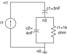
A net-list of an analogue circuit can be con-structed by declaring system variables of type node and analogue components as shown below of the loop filter in a phase locked loop (explained later in Sec-tion 5). Fig 3 shows its corresponding schematic. The circuit’s data base is constructed once, prior to a simulation.
sc_a_node n1("n1"), n2("n2"), n0("n0"); sc_a_currentS I1("I1",n1,n0,&Iin); sc_a_capacitor c1("c1",n1,n2,3e-9); sc_a_resistor r1("r1",n2,n0,1e3); sc_a_capacitor c2("c2",n2,n0,4e-9);
n1
n0 n2 I1
c1=3nF
c2= 4nF
[image:3.595.326.532.169.399.2]r1=1k ohm
Figure 3: Schematic of the loop filter in PLL exam-ple.
2.3 Virtual Build Method
Thebuildmethod specifies the analogue behaviour of a component. This is a virtual method with a default body in the abstract component base class and inherited by all derived components. Thebuild
method consists of C++ code which defines one or more DAEs. For example, Fig. 4 shows the ca-pacitor representation. The figure shows the capac-itor’s differential equation, its representation after discretisation and part of the corresponding build
method. The resulting Jacobian stamp conforms to the Modified Nodal Analysis formulation MNA. Calls to BuildRhs, build the differential equations for the capacitor or the right hand side RHS. Calls
to BuildM, which build the corresponding Jacobian entries are optional. If these calls are not provided, the solver will build the Jacobian using a secant ap-proach with finite difference approximation of the Ja-cobian entries. The entire equation set is formulated automatically at each Newton-Raphson iteration by scanning the linked list of components and invoking their build methods.
void capacitor::build(void){ ...
S=Sn();
CVdotn=C*S*(Xdot(a)-Xdot(b));
BuildM(a,a,S*C); BuildM(a,b,-S*C); BuildM(b,a,-S*C); BuildM(b,b,S*C);
BuildRhs(a,-CVdotn); BuildRhs(b,CVdotn); }
(
−1, −1,...)
+ =
= ab abn abn abn abn
ab SCv CX v v
dt dv C
i &
− − +
+ + − − = ∆ ⋅
−
−
+
n n n n
n n n n
n SCva CXa SCvb CXb CXb SCvb CXa SCva v
SC SC
SC SC
1
RHS v Jacobian.∆ =
Va
a Vb
b
a b
[image:3.595.103.237.441.550.2]C
Figure 4: Capacitor equation and build function.
3
DIGITAL-ANALOGUE
INTERACTION
Connectivity between analogue and digital models requires special consideration since the two mod-els have different language representations. The so-lution to this problem is to insert a special inter-face model directly between the digital and analogue parts. The intended interfacing solution is similar to those adopted in VHDL-AMS and Verilog-AMS. A/D and D/A interfaces are used only to change rep-resentations of signals between the digital and ana-logue domains.
3.1 Digital-Analogue Interface
shown in Fig. 5. This method is capable of handling small time step size as well.
Sn=
Snhn+τ S0n−1
τ+hn
(2)
where Sn is the input digital signal of type bool.
hn is the simulation time step size. Sn0 is the
smoothed signal and S0
n−1 is the past value of the smoothed signal. τ is time constant which plays as a control factor to shape the signal.
Digital World Analog World smoothing
t
tn
n
S
t
-t+
[image:4.595.79.264.221.295.2]Event on signal Sn
Figure 5: Handling small time step sizes.
3.2 Analogue-Digital Interface
interfaceAD is a SystemC module takes analogue signal of typedoubleand produce a digitalbool sig-nal. The criteria to generate a digital event is sim-ple, if the threshold voltage E defined is exceeded, an event with a state (high) is generated. An event with a state (low) is produced, if the analogue volt-age falls below the threshold voltvolt-age. Due to the fact that the result is a digital boolean signal, an event is to be generated at every signal change. The digital part will react to this event if a concurrent statement reads this signal or if the sensitivity list of a process contains this signal.
3.3 Analogue Stepping
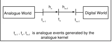
The time step of the analogue simulator is deter-mined by the internal algorithm of the simulator, which means it cannot be defined by the user. Ana-logue simulators do not use events but instead em-ploy an entirely different approach to time step con-trol, namely, continuous step size adjustment, as il-lustrated in Fig. 6, whereh=hn, hn+1, ...may have different values.
Digital World Analogue World
hn hn+1
tn-1 tn tn+1
tn-1, tn, tn+1 is analogue events generated by the
analogue kernel
Figure 6: Analogue stepping.
The implementation of analogue stepping is based on the estimation of the Local Truncation
Er-ror LTE. LTE at tn is an error due to a numerical
approximation introduced in the time pointtn.
In order to synchronise the analogue and digital simulators at every time point, the analogue step-ping is done in SystemC using event notifications. The analogue kernel which is responsible for cal-culating the estimated value of the upper step size boundhn notifies the kernel at the time point equal
tosc_time_stamp()+hn. The digital processes will
be activated at this time point accordingly.
4
TIME SYNCHRONISATION
BETWEEN ANALOGUE AND
DIGITAL SOLVERS
The most important problem in mixed-signal simu-lation is the time synchronisation between the event-driven digital simulation and the numerical integra-tion in the analogue simulaintegra-tion. Synchronisaintegra-tion is a key issue affecting the simulation speed and ac-curacy. Illustrated in the following sections the Sys-temC simulation cycle and the way our analogue ker-nel is linked to it.
4.1 SystemC Simulation cycle
Like in the case of most high-level HDLs, a SystemC model consists of a hierarchical network of parallel processes, which exchange messages under the con-trol of the simulation kernel process [3] and concur-rently update the values of signals and variables. Sig-nal assignment statements do not affect the target signals immediately, but the new values become ef-fective in the next simulation cycle [8]. The kernel process resumes when all the user defined processes become suspended either by executing await state-ment or upon reaching the last process statestate-ment. On resumption, the kernel updates the signals and variable and suspends again while the user processes resume. If the time of the next earliest event tn is
equal to the current simulation timetc, the user
pro-cesses execute a delta cycle.
4.2 Proposed Mixed-Signal SystemC
Simulation cycle
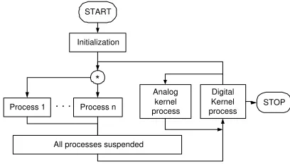
In this proposed research, the digital and analogue simulation cycles are combined. Hence, a set of computations of the analogue equations is executed between the digital evaluation points. To comply with the SystemC execution semantics, the proposed mixed-signal simulator comprises an analogue kernel (see Fig. 7), which runs as a SystemC process and drives the user defined analogue modules.
[image:4.595.81.262.653.722.2]Initialization
*
Process 1
Analog kernel process
Digital Kernel process
All processes suspended . . .
START
[image:5.595.67.271.66.182.2]STOP Process n
Figure 7: The proposed simulation cycle of a Sys-temC system with analogue kernel.
step size adjustment to minimize the errors caused by the numerical integration method.
It is therefore necessary for the analogue kernel in a SystemC environment to handle delta cycles in a manner similar to that of digital processes. However, the state of the analogue solver may not be updated until after the SystemC kernel advances the simu-lation time ahead of the current simusimu-lation timetc,
unless a delta cycle occurs and reevaluation of the current step is necessary.
The technique used in this project for synchro-nisation is the lock-step one. The analogue simula-tor calculates the step sizes and the digital simulasimula-tor uses these values. The analogue kernel advances until the current simulation time and, before suspending, schedules an event at the time equal to the current simulation time plus the next selected step size. The method has been implemented in the extended lan-guage by modifying the SystemC kernel specified by (sc simcontext.cpp) from the SystemC library.
5
CASE STUDY: 2GHZ PHASE
LOCKED LOOP
To verify the functionality of the proposed SystemC mixed-signal simulator, a case study of modelling a 2GHz Phase Locked Loop (PLL) is illustrated. PLL is non-trivial system to model. Systems of this kind usually put standard SPICE-like simulators into dif-ficulties because of the disparate time scales of their transients. As a typical simulation in a system of this kind might require a hundred million time points, ex-cessive CPU times often occur when the entire sys-tem is modelled on the circuit level. The capacity of SystemC to enable system level mixed-signal mod-elling can vastly reduce simulation times where con-cepts need to be verified quickly and detailed circuit level modelling is not required. Fig. 8 shows a block diagram of the modelled PLL.
Phase
Detector LPF VCO
Divide by 2000
Charge Pump
f vco 2GHz
f div
fref
1MHz up Inoise
down
[image:5.595.326.529.68.193.2]noise source
Figure 8: 2GHz Phase Locked Loop with noise and jitter.
5.1 Noise Module
One of the major concerns in the design of PLLs is noise and jitter performance. For example in transceiver designs, jitter from a PLL directly acts to degrade the noise floor and the selectivity of the transceiver. Jitter is modelled here as a Gaussian process with zero mean. It is assumed that only the charge pump was subject to jitter and its signal can be expressed as in Eq. 3,
Inoisy=I(t+J itter(t)) (3)
PLL noise behaviour is difficult to predict with traditional circuit simulators because a PLL gener-ates repetitive switching events as an essential part of its operation, and the noise performance must be evaluated in time-domain when large signals are present. Most classical simulators, SPICE being the best example, are not capable to simulate noise in PLLs. Using the extended SystemC, suitable noise modules can be constructed with no difficulty. The noise module here relies on the standard C++ ran-dom number generator functionrand()and includes a Box-Muller converter of uniform random numbers to Gaussian distribution.
5.2 Voltage-Controlled Oscillator
The VCO generates a square wave whose frequency is proportional to the input signal level. The VCO frequency is the rate of change of the phase (Eq. 4),
˙ϕ(t) = dϕ
dt =f(v) =fc+df∗Vf ilter (4)
Where Vf ilter is the output voltage of the loop
filter, fc is the center frequency of the VCO, and
df= fmax−fc
Vmax is the VCO gain. The VCO was
the VCO contribution to the system jacobian. Equa-tion classes such as VCO class are inherited from the component class so that it allocates its place in the jacobian. Part of the VCO class is shown below:
vco::vco(char nameC[5],SystemVariable *node_a, sc_signal<bool> *Vout): component(nameC,node_a, 0, value){
Vco=Vout;
phi = new sc_a_free_variable("phi"); }
void vco::build(void){ ... phase = X(phi); phase=fmod(phase,1.0); if(phase > 1.0)
PhaseNoisy = phase + Pnoise; if (PhaseNoisy > 0.5)
Vco->write(true); if (PhaseNoisy < 0.5) Vco->write(false);
double fmin=0.5e9, fmax=5e9, Vmax=3.3, df, fc=2e9; df= (fmax-fc) / Vmax;
double S, Qdotn, freq; S=Sn();
Qdotn=Xdot(phi);
freq = fc + df * (a->readn());
if (freq < fmin || freq> fmax) {
if (freq < fmin ) freq = fmin; else freq = fmax;
BuildM(phi,phi,S); BuildM(phi,a,0);
BuildRhs(phi,-Qdotn + fc + (a->readn()) * df); }
else{
BuildM(phi,phi,S); BuildM(phi,a,-df);
BuildRhs(phi,-Qdotn + fc + (a->readn()) * df); }
}
5.3 Simulation
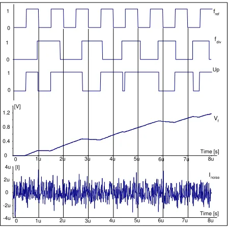
[image:6.595.317.541.59.282.2]The system was simulated with extremely small ana-logue steps which are required to accurately reflect the effects of noise and jitter. To enforce a step size of 10ps or less, the charge pump module is sensitive to a 100GHz clock, whereas the digital modules are sensitive only to their input signals. Fig. 9 shows dif-ferent system values in the first micro seconds of the simulation. Table 1 shows some simulation figures.
Table 1: PLL simulation figures Simulation time 200µSec Number of steps 20 Millions
CPU time 1157.37 Sec
6
CONCLUSION
A mixed-signal simulator based on SystemC has been developed to simulate a general analogue and mixed-signal systems modelled at different abstraction lev-els. The proposed simulator achieved a good results and capable of operations, some recent simulators are unable to perform. Operations such as noise analy-sis, reasonable CPU time even with 20 Million time
fdiv fref
Up
Inoise
-4u -2u 0 2u
4u [I]
0 1u 2u 3u 4u 5u 6u 7u Time [s]8u
Vf
0 0.4 0.8 1.2
0 1u 2u 3u 4u 5u 6u 7u 8u
[V]
Time [s] 0
1 0 1 0 1
Figure 9: 2GHz Synthesizer simulation results.
steps and modelling at different levels in the same design. The extension is still under further develop-ment and is aiming to cover more AMS aspects and more case studies.
References
[1] Pichon F. Blanc S. and Candaele B., “Mixed-signal modelling in vhdl for system-on-chip ap-plications,” in European Design and Test
Con-ference, Paris, France, 6-9 March 1995, pp. 218–
222.
[2] Celoxica, Survey of System Design Trends, De-cember 2003.
[3] Open SystemC Initiative OSCI Documents,
Sys-temC Language Reference Manual, 2003.
[4] Einwich K. Clauss Ch. Noessing G. Schwarz P. and Zojer H., “Systemc extensions for mixed-signal system design,” inFDL, Lyon France, 3-7 September 2001.
[5] Bonnerud T. Hernes B. and Ytterdal T., “A mixed-signal functional level simulation frame-work based on systemc,” in CICC, San Diego California USA, 6-9 May 2001.
[6] Conti M. Caldari M. Orcioni S. and Biagetti G., “Analog circuit modelling in systemc,” inFDL, Frankfurt, Germany, 23-26 September 2003.
[7] Grimm Ch. Meise Ch. Heupke W. and Wald-schmidt K., “Refinement of mixed-signal systems with systemc,” in DATE, Messe Munich, Ger-many, 3-7 March 2003.
[image:6.595.59.261.144.442.2]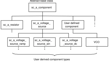
![4 {(E) 2 [4 (But 3 en 1 yloxy)phenyl]diazen 1 yl}benzoic acid](data:image/gif;base64,R0lGODlhAQABAIAAAP///wAAACH5BAEAAAAALAAAAAABAAEAAAICRAEAOw==)