Kernel Based Learning of Hierarchical Multilabel Classification Models

Kernel-Based Learning of

Hierarchical Multilabel Classification Models

∗

Juho Rousu [email protected]

Department of Computer Science PO Box 68

FI-00014 University of Helsinki, Finland

Craig Saunders [email protected]

Sandor Szedmak [email protected]

John Shawe-Taylor [email protected]

Electronics and Computer Science University of Southampton SO17 1BJ, United Kingdom

Editors: Kristin P. Bennett and Emilio Parrado-Hern´andez

Abstract

We present a kernel-based algorithm for hierarchical text classification where the documents are allowed to belong to more than one category at a time. The classification model is a variant of the Maximum Margin Markov Network framework, where the classification hierarchy is represented as a Markov tree equipped with an exponential family defined on the edges. We present an effi-cient optimization algorithm based on incremental conditional gradient ascent in single-example subspaces spanned by the marginal dual variables. The optimization is facilitated with a dynamic programming based algorithm that computes best update directions in the feasible set.

Experiments show that the algorithm can feasibly optimize training sets of thousands of exam-ples and classification hierarchies consisting of hundreds of nodes. Training of the full hierarchical model is as efficient as training independent SVM-light classifiers for each node. The algorithm’s predictive accuracy was found to be competitive with other recently introduced hierarchical multi-category or multilabel classification learning algorithms.

Keywords: kernel methods, hierarchical classification, text categorization, convex optimization, structured outputs

1. Introduction

In many application fields, taxonomies and hierarchies are natural ways to organize and classify objects, hence they are widely used for tasks such as text classification. In contrast, machine learn-ing research has largely been focused on flat target prediction, where the output is a slearn-ingle binary or multivalued scalar variable. Naively encoding a large hierarchy either into a series of binary problems or a single multiclass problem with many possible class values suffers from the fact that dependencies between the classes cannot be represented well. For example, if a news article be-longs to category MUSIC, it is very likely that the article belongs to category ENTERTAINMENT. The failure to represent these relationships leads to a steep decline of the predictive accuracy in the

number of possible categories. In recent years, methods that utilize the hierarchy in learning the classification have been proposed by several authors (Koller and Sahami, 1997; McCallum et al., 1998; Dumais and Chen, 2000). Very recently, new hierarchical classification approaches utilizing kernel methods have been introduced (Hofmann et al., 2003; Cai and Hofmann, 2004; Dekel et al., 2004). The main idea behind these methods is to map the documents (or document–labeling pairs) into a potentially high-dimensional feature space where linear maximum margin separation of the documents becomes possible.

Most of the above mentioned methods assume that the object to be classified belongs to exactly one (leaf) node in the hierarchy. In this paper we consider the more general case where a single object can be classified into several categories in the hierarchy, to be specific, the multilabel is a union of partial paths in the hierarchy. For example, a news article about David and Victoria Beckham could belong to partial pathsSPORT,FOOTBALLandENTERTAINMENT,MUSICbut might not belong to any leaf categories such asCHAMPIONS LEAGUE. The problem of multiple partial paths was also considered in Cesa-Bianchi et al. (2004).

Recently Taskar et al. (2003) introduced a maximum margin technique which optimized an SVM-style objective function over structured outputs. This technique used a marginalization trick to obtain a polynomial sized quadratic program using marginal dual variables. This was an im-provement over the exponentially-sized problem resulting from the dualization of the primal margin maximization problem, which only can be approximated with polynomial number of support vectors using a working set method (Altun et al., 2003; Tsochantaridis et al., 2004).

Even using marginal variables, however, the problem becomes infeasible for even medium sized data sets. Therefore, efficient optimization algorithms are needed. In this paper we present an algo-rithm for working with the marginal variables that is in the spirit of Taskar et al. (2003), however a reformulation of the objective allows a conditional-gradient method to be used which gains effi-ciency and also enables us to work with a richer class of loss functions.

The structure of this article is the following. In Section 2 we present the classification frame-work, review loss functions and derive a quadratic optimization problem for finding the maximum margin model parameters. In Section 3 we present an efficient learning algorithm relying a decom-position of the problem into single training example subproblems and conducting iterative condi-tional gradient ascent in marginal dual variable subspaces corresponding to single training examples. A dynamic programming algorithm is presented that used to efficiently find the best update direc-tions. Extensions and variants are briefly discussed in Section 4. We compare the new algorithm in Section 5 to flat and hierarchical SVM learning approaches and the hierarchical regularized least squares algorithm recently proposed by Cesa-Bianchi et al. (2004). We conclude the article with discussion in Section 6.

2. Maximum Margin Hierarchical Multilabel Classification

We consider data from a domain

X

×

Y

where

X

is a set and

Y

=

Y

1× · · · ×

Y

k is a Cartesian product of the sets

Y

j={+1,−1},j=1, . . . ,k. A vector y= (y1, . . . ,yk)∈

Y

is called the multilabel and the components yjare called the microlabels.

We assume that a training set{(xi,yi)}mi=1⊂

X

×

Y

has been given, consisting of training

A HUMAN NECESSITIES

A 01 AGRICULTURE; FORESTRY; ANIMAL HUSBANDRY; . . . A 01 B SOIL WORKING IN AGRICULTURE OR FORESTRY

A 01 B 1/02 Spades; Shovels

A 01 B 9/00 Ploughs with rotary driven tools D TEXTILES; PAPER

D 21 PAPER-MAKING; PRODUCTION OF CELLULOSE D 21 F PAPER-MAKING MACHINES

D 21 F 1/00 Wet end of machines for making continuous webs of paper

E.C.1 Oxidoreductases

E.C.1.1. Acting on the CH-OH group of donors.

E.C.1.1.1 With NAD(+) or NADP(+) as acceptor. E.C.1.1.1.1 Alcohol dehydrogenase. E.C.6 Ligases

E.C.6.1 Forming carbon-oxygen bonds.

E.C.6.1.1 Ligases forming aminoacyl-tRNA and related compounds. E.C.6.1.1.1 Tyrosine–tRNA ligase.

Figure 1: Examples of classification hierarchies: An excerpt from the WIPO patent classification hierarchy (top) and an excerpt from the Enzyme Classification scheme (bottom).

As the model class we use the exponential family

P(y|x) = 1

Z(x,w)_e

∏

_∈Eexp w

T

eφe(x,ye)

= 1

Z(x,w)exp w

T_φ(x,y)

defined on the edges of a Markov tree T= (V,E), where node j∈V corresponds to the j’th

compo-nent of the multilabel and the edges e= (j,j′)∈E correspond to the classification hierarchy given

as input. Above, Z(x,w) =∑yexp wTφ(x,y)

is the normalizing factor also called the partition function. By ye= (yj,yj′)we denote the restriction of the multilabel y= (y1, . . . ,y_k) to the edge

e= (j,j′). By

Y

e=

Y

j×

Y

j′ we denote the set of labelings of an edge e= (j,j′).

In this work, we assume that the Markov tree T is given a priori. This is a reasonable assumption, as hand-made hierarchies and taxonomies are frequent in applications. The ability to learn the structure from data is an important and challenging question, which is out of scope of this article (See Lafferty et al. (2004) for a study to that direction).

Figure 1 depicts examples of two hierarchical classification domains, patent classification ac-cording to the World International Patent Organization (WIPO) that is used to classify patent texts, and enzyme classification scheme (EC) used by biologists to classify amino acid sequences for enzymatic proteins.

2.1 Loss Functions for Hierarchical Multilabel Classification

though. The loss function between two multilabel vectors y and u should obviously fulfill some basic conditions:ℓ(u,y) =0 if and only if u=y,ℓ(u,y)is maximum when uj6=yjfor every 1≤j≤

k, andℓshould be monotonically non-decreasing with respect to the sets of incorrect microlabels. These conditions are satisfied by, for example, zero-one lossℓ_0/1(y,u) = [y6=u].However, it gives loss of 1 if the complete hierarchy is not labeled correctly, even if only a single microlabel was predicted incorrectly.

In multilabel classification, we would like the loss to increase smoothly so that we can make a difference between ’nearly correct’ and ’clearly incorrect’ multilabel predictions. Symmetric

differ-ence loss

ℓ_∆(y,u) =

∑

j

[yj6=uj],

has this property and is an obvious first choice as the loss function in structured classification tasks. However, the classification hierarchy is not reflected in any way in the loss. For uni-category hierarchical classification (Hofmann et al., 2003; Cai and Hofmann, 2004; Dekel et al., 2004), where exactly one of the microlabels has value 1, Dekel et al. (2004) use as a loss function the length of the path (i1,· · ·,ik) between the the true and predicted nodes with positive microlabels

ℓPAT H(y,u) =|path(i : yi=1,j : uj=1)|. Cai and Hofmann (2004) defined a weighted version of the loss that can take into account factors such as subscription loads of nodes.

In the union of partial paths model, where essentially we need to compare a predicted tree to the true one the concept of a path distance is not very natural. We would like to account for the incorrectly predicted subtrees—in the spirit ofℓ∆—but taking the hierarchy into account. Predicting the parent microlabel correctly is more important than predicting the child correctly, as the child may deal with some detailed concept that the user may not be interested in; for example whether a document was about CHAMPIONS LEAGUEfootball or not may not relevant to a person that is interested in FOOTBALL in general. Also, for the learners point of view, if the parent class was already predicted incorrectly, we don’t want to penalize the mistake in the child. A loss function that has these properties was given by Cesa-Bianchi et al. (2004). It penalizes the first mistake along a path from root to a node

ℓH(y,u) =

∑

j

cj[yj6=uj & yh=uh∀h∈anc(j)],

where anc(j)denotes the set of ancestors of node j. The coefficients 0≤cj≤1 are used for down-scaling the loss when going deeper in the tree. These can be chosen in many ways. One can divide the maximum loss among the subtrees met along the path. This is done by defining

croot =1,cj=cpa(j)/|sibl(j)|,

where we denoted by pa(j) the immediate parent and by sibl(j)the set of siblings of node j (in-cluding j itself). Another possibility is to scale the loss by the proportion of the hierarchy that is in the subtree T(j)rooted by j, that is, to define

cj=|T(j)|/|T(root)|.

Using ℓH for learning a model has the drawback that it does not decompose very well: the labelings of the complete path are needed to compute the loss. Therefore, in this paper we consider a simplified version ofℓH, namely

ℓH˜(y,u) =

∑

j

cj[yj6=uj & ypa(j)=upa(j)],

that penalizes a mistake in a child only if the label of the parent was correct. This choice leads the loss function to capture some of the hierarchical dependencies (between the parent and the child) but allows us define the loss in terms of edges, which is crucial for the efficiency of our learning algorithm.

Using the above, the per-microlabel loss is divided among the edges adjacent to the node. This is achieved by defining an edge-lossℓe(ye,ue) =ℓj(yj,uj)/

N

(j) +ℓj′(y_j′,u_j′)/

N

(j′)for each e=

(j,j′), where ℓj is the term regarding microlabel j, ye= (yj,yj′) is a labeling of the edge e and

N

(j)denotes the neighbors of node j in the hierarchy (i.e. the children of a nodes and it’s parent). Intuitively, the edges adjacent to node j ’share the blame’ of the microlabel lossℓj. The multilabel loss (ℓ_∆orℓ_H˜) is then written as a sum over the edges:ℓ(y,u) =∑e∈Eℓe(ye,ue).

The above described loss functions do not represent an exhaustive list of the possible ones. With probabilistic models, it is common to employ KL-divergence or negative log likelihood as the loss function (Lafferty et al., 2004). In the max-margin learning framework these types of loss functions are not applicable, as they require estimating the underlying probability distribution, e.g. to compute the log-partition function. As our central theme is efficient computation of structured prediction models, we concentrate on the above simpler formulations of loss functions.

2.2 Feature Representations for Structured Inputs

When handling input data that already comes in vector form, there is no obligation to introduce a special kernel function. The inner product of the inputs K(x,z) =xTz, also called the ’linear kernel’,

can be used. However, when using structured data such as sequences, trees or graphs, one needs to convert the structured representation to a vector form. Feature representation for structured input data have been considered in many works already (c.f. Gartner (2003)), we will concentrate to the important case of hierarchical classification of text or, in general, sequence data.

For sequences the most common feature representation is to count or check the existence of sub-sequence occurrences, when the subsub-sequences are taken from a fixed index set U . Different choices for the index set and accounting for occurrences give rise to a family of feature representations and kernels. Below we review the main forms of representation for sequences and the computation kernels for such representations.

Word spectrum (Bag-of-words) kernels. In the most widely used feature representation for strings in a natural language, informally called bag-of-words (BoW), the index set is taken as the set of words in the language, possibly excluding some frequently occurring stop words (Salton, 1989). The representation was brought to SVM learning by Joachims (1998).

In the case of a string s containing English text, for each English word u, we define the feature value

φu(s) =|{j|sj. . .sj+|u|−1=u}|,

φdog(s) =1, φwas(s) =1, φchased(s) =1, φby(s) =1, φfat(s) =1, φcat =1. These occurrence counts can also be weighted, for example by scaling by the inverse document frequency as is done in TFIDF weighting (c.f. Salton (1989)):

φu(s) =|{j|sj. . .sj+|u|−1=u}| ×log2N/Nu,

where Nuis the number of documents where u occurs and N is the total number of documents in the collection.

Although the dimension of the feature space may be high, computation of the BoW kernel can be efficiently implemented by scanning the two strings, constructing lists L(s) and L(t) of pairs (u,cu)of word u and occurrence count cuordered in the lexicographical order of the substrings u, and finally traversing the two lists to compute the dot product.

Substring spectrum kernels. For strings that do not encompass a crisply defined word-structure, for example, biological sequences, a different approach is more suitable. Given an alphabetΣ, a simple choice is to take U =Σp_{, the set of strings of length p. In some cases, using a range of} substring lengths q≤l≤p may be more appropriate than picking a single length. We can define

U=Σq∪Σq+1· · · ∪Σpfor some 1≤q≤p.

The most efficient approaches, working in O(p(|s|+|t|))time, to compute substring spectrum kernels are based on suffix trees (Leslie et al., 2002; Vishwanathan and Smola, 2002), although dynamic programming and approaches based on the trie data structure also can be used Shawe-Taylor and Cristianini (2004).

The substring kernels can be generalized in many ways, for example

• Gapped substring spectrum kernels allow gaps in the subsequence occurrences. Gap-weighting

can be used to down-weight substring occurrences that contain many or long gaps (Lodhi et al., 2002; Rousu and Shawe-Taylor, 2005).

• Word or syllable alphabets can be used in place of characters (Saunders et al., 2002; Cancedda

et al., 2003).

2.3 Feature Representations for Hierarchical Outputs

When the input features are used in hierarchical classification, they need to be associated with the labelings of the hierarchy. In our setting, this is done via constructing a joint feature map φ:

X

×

Y

7→

F

xy. There are important design choices to be made in how the hierarchical structure should reflect in the feature representation.

There are two general types of features that can be distinguished:

Global features are given by the feature mapφx:

X

7→

F

x. They are not tied to a particular vertex or edge but represent the structured object as a whole. For example, the bag-of-words or the substring spectrum of a document is not tied to a single class of documents in a hierarchy, but a given word can relate to different classes with different importances.

Given the input features, there are two basic ways by which the joint feature vector can be con-structed:

Orthogonal feature representation is defined asφ(x,y) = (φ_e(x,ye))e∈E,so that there is a block for each edge (or vertex), which, in turn, is divided into blocks for a specific edge-labeling pairs(e,ue), i.e.φe(x,ye) = (φuee(x,ye))_ue∈Ye.

The vector φu_e should incorporate both the x-features relevant to the edge and encode the dependency on the labeling of the edge. A simple choice is to define

φue

e (x,ye) = [ue=ye] φx(x)T,φxe(x)T

T

that incorporates both the global and local features if the edge is labeled ye=ue, and a zero vector otherwise. Intuitively, the features are turned ’on’ only for the particular labeling of the edge that is consistent with y.

Additive feature representation is defined as

φ(x,y) =

∑

e∈Eu

∑

e∈Ye

[ye=ue]φuee(x),

whereφue

e contains features specific to the pair(e,ue).

The orthogonal and additive feature representations differ from each other in several respects. In the orthogonal representation, global features get weighted in a context-dependent manner: some features may be more important in labeling one edge than another. Thus, the global features will be ’localized’ by the learning algorithm. The size of the feature vectors grow linearly in the number of edges, which requires careful implementation if solving the primal optimization problem (1) instead of the dual. The kernel induced by the above feature map decomposes as

K(x,y; x′,y′) =

∑

e∈E

φ_e(x,ye)Tφe(x′,y′e) =

∑

e∈E

Ke(x,ye; x′,y′e),

which means that there is no crosstalk between the edges:

φe(x,ye)Tφe′(x,y_e′) =0

if e6=e′, hence the name ’orthogonal’. The number of terms in the sum when calculating the kernel obviously scales linearly in the number of edges.

The dimension of the feature vector using the additive feature representation is independent of the size of the hierarchy, thus optimization in primal representation (1) is more feasible for large structures. Second, as there are no feature weights depending on a particular part of the structure, the existence of local features is mandatory, otherwise the output structure is not reflected in the feature vector. Third, the kernel

K(x,y; x′,y′) =

∑

e

φe(x,y)

T

∑

e

φe(x′,y′)

=

∑

e,e′

φ_e(x,ye)Tφe′(x,y′_e′) =

∑

e,e′

induced by this representation typically has non-zero blocks Kee′ 6=0, representing cross-talk

between edges. There are two consequences of this fact. First, the kernel does not exhibit the sparsity that is implied by the hierarchy, thus it creates the possibility of overfitting. Second, the complexity of the kernel will grow quadratically in the size of the hierarchy rather than linearly as is the case with orthogonal features. This is another reason why a primal optimization approach for this representation might be more justified than a dual approach.

In the sequel, we describe a method that relies on the orthogonal feature representation which will give us a dual formulation with complexity growing linearly in the number of edges in E. The kernel defined by the feature vectors, denoted by

Kx(x,x′) =φx(x)Tφx(x′),

is referred to as x-kernel while K(x,y; x,y′)is referred to as the joint kernel.

2.4 Maximum Margin Learning

Typically in learning probabilistic models, one aims to learn maximum likelihood parameters, which in the exponential CRF amounts to solving

argmax_wlog m

∏

i=1

P(yi|xi; w)

!

=argmax_w m

∑

i=1

wTφ(xi,yi)−log Z(xi,w)

.

This estimation problem is hampered by the need to compute the (logarithm of the) partition func-tion Z. For a general graph this problem is hard to solve. Approximafunc-tion methods for its compu-tation is a subject of active research (c.f. Wainwright and Jordan 2003). Also, in the absence of regularization the max-likelihood model is likely to suffer from overfitting

An alternative formulation (c.f Altun et al. 2003; Taskar et al. 2003), inspired by support vector machines, is to estimate parameters that in some sense maximize the ratio

P(yi|xi; w)

P(y|xi; w)

between the probability of the correct labeling yi and the worst competing labeling y. With the exponential family, the problem translates to the problem of maximizing the minimum linear margin

wTφ(xi,yi)−wTφ(xi,y)

in the log-space.

Furthermore, we would like the marginγto scale as a function of the loss so that grossly incor-rect pseudo-examples are pushed farther from the corincor-rect labeling than only slightly incorincor-rect ones. Using the canonical hyperplane representation (c.f. Cristianini and Shawe-Taylor (2000)) this can be stated as the following minimization problem:

min

w

1 2||w||

2

where∆φ(xi,y) =φ(xi,yi)−φ(xi,y). As with SVMs, a model satisfying margin constraints exactly rarely exists, hence it is necessary to add slack variablesξi to allow examples to deviate from the margin boundary. Altogether, this results in the following optimization problem

min

w

1 2||w||

2 +C

m

∑

i=1

ξi

s.t. wT∆φ(xi,y)≥ℓ(yi,y)−ξi,∀i,y. (1)

This optimization problem suffers from the possible high-dimensionality of the feature vectors, for example with string kernels, and from the exponential-sized constraint set (in the length of the multilabel vector). A dual problem

max

α≥0 α

T_ℓ−1 2α

T_{Kα, s.t.}

∑

y

α(i,y)≤C,∀i, (2)

where K=∆ΦT_{∆Φis the joint kernel matrix for pseudo-examples(x}

i,y)andℓ= (ℓ(yi,y))i,yis the

loss vector, allows us to circumvent the problem with feature vectors. However, in the dual problem there are exponentially many dual variablesα(i,y), one for each pseudo-example.

There are a few basic routes by which the exponential complexity can be circumvented:

• Dual working set methods where the constraint set is grown incrementally by adding the worst margin violator

argmin_i,ywT∆φ(xi,y)−ℓ(yi,y)

to the dual problem. One can guarantee an approximate solution with a polynomial number of support vectors by this approach (Altun et al., 2003; Tsochantaridis et al., 2004).

• Primal methods where the solution above inference problem is integrated to the primal opti-mization problem, rather than writing down the exponential-sized constraint set (Taskar et al., 2004).

• Marginal dual methods, where the problem is translated to a polynomial-sized form via con-sidering the marginals of the dual variables (Taskar et al., 2003).

The methodology presented in this article belongs to the third category.

2.5 Marginalized Dual Problem

The feasible set of the dual problem (2) is a Cartesian product

A

=

A

1× · · · ×

A

m (3)

of identical closed polytopes

A

i={αi∈R|Y||αi≥0,||αi||₁≤C}, (4)

The dimension of the set

A

, dA =m|

Y

|is exponential in the length of the multilabel vectors. This means that optimizing directly over the the set

A

is not feasible. Fortunately by utilizing the structure of T , the set

A

can be mapped to a set

M

of polynomial dimension, called the marginal polytope of H, where optimization becomes more feasible (Taskar et al., 2003).

For an edge e∈E of the Markov tree T , and an associated labeling ye, the marginal ofα(i,y) for the pair(e,ye)is given by

µe(i,ye) =

∑

{u∈Yi}

[ye=ue]α(i,u) (5)

where the sum picks up those dual variables α(i,y) that have equal value ue =ye on the edge e. Single node marginals µj(i,yj)are defined analogously.

For the hierarchy T , the vector containing the edge marginals of the example xi, the marginal dual vector, is given by

µ_i= (µe(i,ue))_e∈E,ue∈Ye.

The marginal vector of the whole training set is the concatenation of the single example marginal dual vectors µ= (µ_i)m_i=1.The vector has dimension dM =m∑e∈E|

Y

e|=O(m|E|maxe|

Y

e|). Thus the dimension is linear in the number of the examples, edges and the maximum cardinality of set of labelings of a single edge.

The indicator functions in (5) can be collectively represented by the the matrix ME, ME(e,ue; y) =

[ue=ye],and the relationship between a dual vector alpha and the corresponding marginal vector µ is given by the linear map ME·αi=µiand µ= (ME·αi)m_i=1. The image of the set

A

i, defined by

M

i={µi| ∃αi∈

A

i: MEαi=µi} is called the marginal polytope ofαion T .

The following properties of the set

M

i are immediate: Let

A

i be the polytope of (4) and let

M

i be the corresponding marginal polytope. Then

• the vertex set of

M

iis the image of the vertex set of

A

i:

Vµ,i={µi| ∃αi∈Vi: MEαi=µi}.

• As an image of a convex polytope

A

iunder the linear map ME,

M

iis a convex polytope. These properties underlie the efficient solution of the dual problem on the marginal polytope.

The exponential size of the dual problem (2) can be tackled via the relationship between its feasible set

A

=

A

1× · · · ×

A

mand the marginal polytopes

M

iof each

A

i.

Given a decomposable loss function

ℓ(yi,y) =

∑

e∈E

ℓe(i,ye)

the linear part of the objective satisfies m

∑

i=1y

∑

∈Y

α(i,y)ℓ(i,y) =

m

∑

i=1

∑

y

α(i,y)

∑

e

ℓe(i,ye)

=

m

∑

i=1e

∑

∈Eue

∑

∈Ye

∑

y:ye=ue

α(i,y)ℓe(i,ue) = m

∑

i=1e

∑

∈Eue

∑

∈Ye

µe(i,ue)ℓe(i,ue)

=

m

∑

i=1

whereℓE= (ℓi)mi=1= (ℓe(i,ue))mi=1,e∈E,ue∈Yeis the marginal loss vector.

Given an orthogonal feature representation inducing a decomposable kernel K(x,y; x′,y′) =

∑e∈EKe(x,ye; x′,y′e), the quadratic part of the objective becomes

αKα =

∑

e

∑

i,i′

∑

_y,y′

α(i,y)Ke(i,ye; i′,y′e)α(i′,y′)

=

∑

e

∑

i,i′_u

∑

_e,u′

e

Ke(i,ue; i′,u′e)

∑

y:ye=ue

∑

y′_:y′

e=u′e

α(i,y)α(i′,y′)

=

∑

e

∑

i,i′_u

∑

_e,u′

e

µe(i,ue)Ke(i,ue; i′,u′e)µe(i,u′e)

= µTKEµ,

where KE=diag(Ke,e∈E)is a block diagonal matrix with edge-specific kernel blocks Ke. The objective should be maximized with respect to µ whilst ensuring that there exist α∈

A

satisfying Mαi=µ_i for all i, so that the marginal dual solution represents a feasible solution of the original dual. By the properties outlined above, the feasible set of the marginalized problem is the marginal dual polytope, or to be exact the Cartesian product of the marginal polytopes of single examples (which are in fact equal):

M

=

M

1× · · · ×

M

m

In summary, the marginalized optimization problem can be stated in implicit form as

max µ∈M µ

T_ℓ E−

1 2µ

T_K Eµ

This problem is a quadratic programme with a linear number of variables in the number of training examples and in the number of edges.

For optimization algorithms, an explicit characterization of the feasible set is required. Char-acterizing the polytope

M

in terms of linear constraints defining the faces of the polytope, is for general graphs infeasible. Singly-connected graphs such as trees are an exception: for such graphs the marginal polytope is exactly reproduced by the box constraints

∑

ue

µe(i,ue)≤C,∀i,e∈E,µe≥0 (6)

and the local consistency constraints

∑

yk

µk j(i,yk,yj) =µj(i,yj);

∑

yj

µk j(i,yk,yj) =µk(i,yk). (7)

In this case the size of the resulting constraint set is linear in the number of vertices the graph. Thus for small hierarchies graphs it can be written down explicitly and the resulting optimization problem has linear size in both the number of examples and the size of the graph. Thus the approach can in principle be made to work, although not with off-the-shelf QP solvers (see sections 3 and 5).

{(e,e′_{)∈E×E|e= (j}′_,i),e′_{= (i,j)}. By introduction of these marginal consistency constraints} the optimization problem gets the form

max µ≥0_e

∑

_∈Eµ

T eℓe−

1 2_e

∑

_∈Eµ

T

eKeµe (8)

s.t

∑

ye

µe(i,ye)≤C,∀i,e∈E,

∑

y′

µe(i,(y′,y)) =

∑

y′

µe′(i,(y,y′)), ∀i,y,(e,e′)∈E2,

,

While the above formulation is closely related to that described in Taskar et al. (2003), there are a few differences to be pointed out. Firstly, as we assign the loss to the edges rather than the microlabels, we are able to use richer loss functions than the simple ℓ∆. Secondly, single-node marginal dual variables—the µj’s in (7)—become redundant when the constraints are given in terms of the edges. Thirdly, we have utilized the fact that in our feature representation the ’cross-edge’ values∆φ_e(x,ye)T∆φe′(x′,y′_e′), where e6=e′, do not contribute to the kernel, hence we have a

block-diagonal kernel KE =diag(Ke1, . . . ,Ke|E|),KE(i,e,ue; j,e,ve) =Ke(i,ue; j,ve)with the number of

non-zero entries thus scaling linearly rather than quadratically in the number of edges. Finally, we write the box constraint (6) as an inequality as we want the algorithm to be able to inactivate training examples (see Section 3.2).

Like that of Taskar et al. (2003), our approach can be generalized to non-tree structures. How-ever, for a general graph, the feasible region in (8) will only approximate that of (2), which will give rise to a approximate solution to the primal. To arrive at an exact solution, one should construct the junction tree for the graph and to write down the corresponding constraints for the junction tree. As a caveat, one should note that for dense graphs, the junction tree may be significantly larger than the size of the original structure. Also, in tractable time, finding the maximum likelihood multilabel can only be approximated.

3. Efficient Optimization of the Marginalized Dual Problem

While the above quadratic program is polynomial-sized—and considerably smaller than that de-scribed in Taskar et al. (2003)—it is still easily too large in practice to fit in main memory or to solve by off-the-shelf QP solvers. To arrive at a more tractable problem, we notice from (3) and (4) that the constraint set decomposes by the examples: to satisfy a single box constraint (6) or a marginal consistency constraint (7) one only needs to change the marginal dual variables of a single example. Moreover, the structure of the feasible set only depends on the edge set E, not on the training example in question: we have

A

1=· · ·=

A

m.

However, the kernel matrix only decomposes by the edges as most pairs of examples have non-positive kernel value between them. Thus there does not seem to be a straightforward way to decompose the quadratic programme.

A decomposition becomes possible when considering gradient-based approaches. Let us con-sider optimizing the dual variables µ_i= (µe(i,ye))_e∈E,ye∈Ye of example xiwhereℓidenotes the cor-responding loss vector and Ki j = Ke(i,ue; j,ve)e∈E,ue,ve∈Ye

Obtaining the gradient for the xi-subspace requires computing the corresponding part of the gradient of the objective function in (8) which is gi =ℓi−Ki·µ where ℓi = (ℓe(i,ue))_e∈E,ue∈Ye is the corresponding loss vector for xi. However, when updating µi only, evaluating the change in objective and updating the gradient can be done more cheaply: ∆gi =−Kii∆µi and ∆ob j=

gT_i ∆µ_i−1/2∆µ_iKii∆µ_i.Thus local optimization in a subspace of a single training example can be done without consulting the other training examples. On the other hand, we do not want to spend too much time in optimizing a single example: When the dual variables of the other examples are non-optimal, so is the initial gradient gi. Thus the optimum we would arrive at would not be the global optimum of the quadratic objective. It makes more sense to optimize all examples more or less in tandem so that the full gradient approaches its optimum as quickly as possible.

Before presenting the pseudocode of our method some notations have to be introduced. The function f()denotes the objective function and

F

stands for the set of the feasible solutions in (8). The feasibility domain for µ_iwhen all other components in µ are fixed is denoted by

F

i.

In our approach, we have chosen to conduct a few optimization steps for each training example using a conditional gradient ascent (see Algorithm 2) before moving on to the next example. The iteration limit for each example is set by using the Karush-Kuhn-Tucker(KKT) conditions as a guideline (see Section 3.2).

The pseudocode of our algorithm is given in Algorithm 1. It takes as input the training data, the edge set of the hierarchy, the loss vectorℓ= (ℓi)mi=1and the constraints defining the feasible region.

The algorithm chooses a chunk of examples as the working set, computes the kernel for each xiand makes an optimization pass over the chunk. After one pass, the gradient, slacks and the duality gap are computed and a new chunk is picked. The process is iterated until the duality gap gets below given threshold.

Note in particular, that the joint kernel is not explicitly computed, although evaluating the gra-dient requires computing the product KEµ. However, we are able to take advantage of the special structure of the feature vectors, repeating the same feature vector in different contexts, see the defi-nition of the edge marginal dual variables (5) and the explanation after, to facilitate the computation using the x-kernel Kx(i,j) =∆φ(xi)T∆φ(xj)and the dual variables only.

3.1 Conditional Subspace Gradient Ascent

The optimization algorithm used for a single example is a variant of conditional gradient ascent (or descent) algorithms (Bertsekas, 1999). The algorithms in this family solve a constrained quadratic problem by iteratively stepping to the best feasible direction with respect to the current gradient. It exploits the fact if µ∗ is an optimum solution of a maximization problem with objective function

f above the feasibility domain

F

i then it has to satisfy the first order optimality condition, i.e., the inequality

∇f(µ_i)(µ_i−µ∗)≥0 (9)

has to hold for any feasible µ_ichosen from

F

i.

Algorithm 1 Maximum margin optimization algorithm for the H-M3 hierarchical classification model.

H-M3(S,E, ℓ,

F

)

Require: Training data S= ((xi,yi))m_i=1, edge set E of the hierarchy, a loss vectorℓ, and the feasi-bility domain

F

.

Ensure: Dual variable vector µ and objective value f(µ).

1: Initialize g=ℓ,ξ=ℓ,dg=∞and OBJ=0.

2: while dg>dgmin & iter<max iter do

3: [W S,Freq] =UpdateWorkingSet(µ,g,ξ);

4: Compute x-kernel values KX,W Swith respect to the working set;

5: for i∈W S do

6: Compute joint kernel block Kiiand subspace gradient gi;

7: [µ_i,∆ob j] =CSGA(µ_i,gi,Kii,

F

i,Freqi);

8: end for

9: Compute gradient g, slacksξand duality gap dg;

10: end while

First we need to find a feasible µ∗which maximizes the first order feasibility condition (9) at a fixed µ_i. It gives a direction potentially increasing the value of objective function f . Then we have to choose a step length,τthat gives the optimal feasible solution as a stationary point along the line segment µ_i(τ) =µ_i+τ∆µ, τ∈(0,1], where∆µ=µ∗−µ_i, starting on the known feasible solution µ_i.

The stationary point is found by solving the equation

d dτ

ℓT_i µ_i(τ)−1/2µ_i(τ)TKiiµi(τ)

=0, (10)

expressing the optimality condition with respect to τ. If τ>1, the stationary point is infeasible and the feasible maximum is obtained atτ=1. In our experience, the time taken to compute the stationary point was typically significantly smaller than time taken to find µ∗_i, depending on the dataset characteristics and the actual algorithm (see Section 3.3) that was used to find µ∗_i.

3.2 Working Set Maintenance

We wish to maintain the working set so that the most promising examples to be updated are con-tained there at all times to minimize the amount of computation used for unsuccessful updates. Our working set update is based on the Karush-Kuhn-Tucker(KKT) conditions which at the optimum hold for all xi:

1. (C−∑e,yeµe(i,ye))ξi=0, and 2. α(i,y)(wTφ(xi,y)−ℓ(yi,y) +ξi) =0.

Algorithm 2 Conditional subspace gradient ascent optimization step.

CSGA(µ_i,gi,Kii,

F

i,maxiteri)

Require: Initial dual variable vector µ_i, gradient gi, constraints of the feasible region

F

i, a joint kernel block Kiifor the subspace, and an iteration limit maxiteri.

Ensure: New values for dual variables µ_iand change in objective∆ob j. 1: ∆ob j=0; iter=0;

2: while iter<maxiter do

3: % find highest feasible point given gi

4: µ∗=argmax_v∈Fi g T i v;

5: ∆µ=µ∗−µ_i;

6: q=gT_i∆µ,r=∆µTKii∆µ; % taken from the solution of (10) 7: τ=min(q/r,1); % clip to remain feasible

8: ifτ≤0 then

9: break; % no progress, stop 10: else

11: µ_i=µ_i+τ∆µ; % update 12: gi=gi−τKii∆µ;

13: ∆ob j=∆ob j+τq−τ2_r/2; 14: end if

15: iter=iter+1;

16: end while

• Non-saturated (∑e,yeµe(i,ye)<C) examples are given priority as they certainly will need to be updated to reach the optimum.

• Saturated examples (∑e,yeµe(i,ye) =C) are added if there are not enough non-saturated ones. The rationale is that the even though an example is saturated, the individual dual variable values may still be suboptimal being equal to 0.

• Inactive (∑e,_yeµe(i,ye) =0) non-violators (ξi=0) are removed from the working set, as they do not constrain the objective.

Another heuristic technique to concentrate computational effort to most promising examples is to favor examples with a large duality gap

∆ob j(µ,ξ) =

∑

i

Cξi+µT_i gi.

As feasible primal solutions always are least as large as feasible dual solutions, the duality gap gives an upper bound to the distance from the dual solution to the optimum. We use the quantity∆i= Cξi+µT_igias a heuristic measure of the work needed for that particular example in order to reach the optimum. Examples are then chosen to the chunk to be updated with probability proportional to

3.3 Finding Update Directions Efficiently

The optimization algorithm described above relies on efficient computation of update directions µ∗_i in the single example subspaces, that is, to solve the constrained linear program

argmax_v∈Fi g T

iv. (11)

A straightforward approach would be to use a linear programming solver, such as the LIPSOL interior point solver. However, a such black-box approach does not utilize the special structure of the problem in any way.

In order to solve this problem efficiently, we first notice two things:

1. A vertex of the feasible set is always among the optimal solutions.

2. Vertices correspond to consistent labelings of the hierarchy. This can be seen from the fact that at the vertex, for each edge µe(i,ye) =C for exactly one yeand µe(i,ue) =0 for ue6=ye, and that the marginal consistency constraints require that for two adjacent edges e′= (j′,j),e′′= (j,j′′) we have µe′(i,y′_e) =C=µ_e′′(i,y′′_e) with matching edge-labelings y_e′ = (y_j′,y_j) and

y′′_e = (yj,yj′′).

Thus instead of solving (11) directly, we can search for the labeling y∗of the hierarchy corre-sponding to an optimal vertex

vmu(y∗)of the feasible set:

argmax_y∈YgTi µ(y) (12)

This problem can be solved efficiently using a dynamic programming inference algorithm, re-viewed in the next section.

3.4 Solving the Inference Problem in Linear Time

When dealing with structured output models, one needs to solve the inference problem

argmax_y∈YgTi µ(y) (13)

to find a multilabel y maximizing the inner product between some (gradient) vector h and the marginal dual variables µ(y) corresponding to y. In our learning scheme this problem is found in two situations,

• when predicting multilabels given a learned model, and

• to find update directions (12).

The algorithm described below can be used for both problems, the only quantity that changes is the gradient gi.

for each subtree the optimal labeling of the subtree, conditioned on fixing the label of the subtree root to+1 or−1.

We denote by Tj= (Vj,Ej)the subtree of T rooted at node j. We need to maintain two quantities during the bottom-up pass:

• The best objective value that can be obtained for the example i in the subtree rooted at node j when the label yj has been fixed. We denote this value by Syj(i,j).

• The best objective value that can be obtained for the subtree rooted by the edge e= (j,j′) when the root node j is fixed to yj. We denote this value by Gyj(i,e).

The two quantities are computed from the recurrences

Syj(i,j) =

(

∑e=(j,j′_)∈E

jGyj(i,e), if Ej6= /0,and

0, otherwise,

and

Gyj(i,e) =max y_j′

ge(i,yj,yj′)µ_e(i,y_j,y_j′) +S_y

j′(i,j

′₎

At the root node of the hierarchy, maxySy(i,root)finally gives the optimum. The corresponding vertex v(y∗)is found in making a top-down pass over the hierarchy: one looks for best label for a child of a node given the parent has been fixed. It should be noted that although in principle the best conditional labeling—how to label a subtree when the root is fixed to one of the possible labels— could be computed already during the bottom-up pass, the two pass algorithm, where the labeling is worked out only after the label of the global root of the hierarchy has been found out, is much easier to implement and works just as fast.

The dynamic programming scheme can be implemented in vectorized form so that all examples and all nodes on a level of the hierarchy are handled at the same time, thus eliminating the need for loops going over examples and nodes, which in MATLAB implementation are to be avoided.

All in all, the above described inference algorithm works in linear time in the number of dual variables, which can be seen from the fact that each example is processed once, each edge is visited twice (once in the bottom-up pass, once in the top-down pass) and the max operations are taken over the dual variables belonging to the current edge.

3.5 Computing Stationary Points in Linear Time

The conditional gradient ascent requires us to iteratively solve (10) forτ, which givesτ=∆µ/∆µKii∆µ.

The potentially expensive part is evaluating the matrix-vector product Kii∆µ=Kiiµ∗−Kiiµi, which trivially could take quadratic time in the number of variables. However, we can keep in mem-ory the vector Kiiµi during the computation, thus it remains to compute Kiiµ∗. Firstly, we no-tice that for a normalized x-kernel, the entries of the joint kernel are given as sums of indicators

4. Extensions and Variants

There are several variations of the multilabel classification models described above.

Slack variables were defined as non-negative and a single variable was allocated per example. Allowing negative slack (c.f.Taskar et al. (2003); Tsochantaridis et al. (2004)) results in the dual equality constraint∑yeµe(i,ye) =C instead of the box constraint. This results in non-sparse models as training points are very likely to have non-zero slack.

Allotting a separate slack variable for each edge is a possibility when the data for some edges can be considered less reliable than the data for others; in such case the unreliable edge can consume required slack without affecting the other edges. From an optimization point of view, edge-based slack variables make the model decompose into separate edge-based quadratic programs and may allow larger models to be optimized.

Partial paths could be used as the basis of the classification model instead of the edges. For each partial path p= (j1, . . . ,jd) one defines a feature vector φp(i,y) = [yp=1|p|]φ(x), where yp = (yj1, . . . ,yjd) is the restriction of the multilabel to the partial path. As the number of

par-tial paths in the hierarchy equals the number of nodes, the resulting feature vectors are actually smaller than the ones defined by edge-labelings. The marginalization of the model by the partial paths works in an analogous way to the edge-marginalization and the same optimization algorithms can be used. The price of the more compact feature representation comes in the form of slightly more complicated consistency constraints and inference: For consistency one needs to ensure that if a partial path p has non-zero path-marginal µp(i,yp), no prefix p′ of p has non-zero marginal

µp′(i,y_p). Correspondingly, the inference algorithms need to make comparisons between a partial

path and its prefixes.

Non-hierarchical models can also be tackled with the above described framework, with a few caveats. First, ensuring global consistency of the marginalized dual is more involved as local consis-tency of edge-marginals does not guarantee existence of a dual variableα(i,y)with those marginals. If the graph is not too dense this problem can be circumvented by computing the clique tree of the graph and making the clique tree locally consistent, and the conditional gradient optimization will work unmodified. However, inference for general graphs is NP-hard so both computing predictions of the model and finding the update directions in the optimization becomes hard. Several schemes to find approximate solutions exist, including loopy belief propagation, semi-definite relaxations and tree-based approximations (Wainwright and Jordan (2003); Wainwright et al. (2003)). Depending on the application, also considering the model in a decomposed form via definition of edge-slack variables (see above) may be justified.

5. Experiments

We tested the presented learning approach on three datasets that have an associated classification hierarchy:

• WIPO-alpha patent dataset (WIPO, 2001). The dataset consisted of the 1372 training and 358 testing document comprising the D section of the hierarchy. The number of nodes in the hierarchy was 188, with maximum depth 3.

• ENZYME classification dataset. The training data consisted of 7700 protein sequences with hierarchical classification given by the Enzyme Classification (EC) system. The hierarchy consisted of 236 nodes organized into a tree of depth three. Test data consisted of 1755 sequences.

In all datasets, the membership of examples in the nodes of the hierarchy is indicated by binary vectors y∈ {+1,−1}k_{. Multiple paths were actually present in one of the datasets, REUTERS,} approximately 8 percent of examples were classified into more than one category.

The two first datasets were processed into bag-of-words representation with TFIDF weighting. No word stemming or stop-word removal was performed. For the ENZYME sequences a length-4 subsequence kernel was used.

We compared the performance of the presented learning approach—below denoted byH-M3—

to three algorithms: SVMdenotes an SVM trained for each microlabel separately,H-SVMdenotes the case where the SVM for a microlabel is trained only with examples for which the ancestor labels are positive.

The SVM and H-SVM were run using the SVM-light package. After pre-computation of the kernel these algorithms are as fast as one could expect, as they just involve solving an SVM for each node in the graph (with the full training set forSVMand usually a much smaller subset forH-SVM).

H-RLSis a batch version of the hierarchical least squares algorithm described in Cesa-Bianchi et al. (2004). It essentially solves for each node i a least squares style problem wi= (I+SiSTi +

xxT₎−1_S

iyi,where Si is a matrix consisting of all training examples for which the parent of node i was classified as positive, yiis a microlabel vector for node i of those examples and I is the identity matrix. Predictions for a node i for a new example x is−1 if the parent of the node was classified negatively and sign(wT_ix)otherwise.

H-RLS requires a matrix inversion for each prediction of each example, at each node along a

path for which errors have not already been made. No optimization of the algorithm was done, except to use extension approaches to efficiently compute the matrix inverse (for each example an inverted matrix needs to be extended by one row/column, so a straightforward application of the Sherman-Morrison formula to efficiently update the inverse can be used).

The H-RLS and H-M3 algorithms were implemented in MATLAB. The tests were run on a high-end PC. For SVM,H-SVM and H-M3, the regularization parameter value C =1 was used in all experiments.

Obtaining consistent labelings. As the learning algorithms compared here all decompose the hierarchy for learning, the multilabel composed of naively combining the microlabel predictions may be inconsistent, that is, they may predict a document as part of the child but not as part of the parent. ForSVM andH-SVMconsistent labelings were produced by post-processing the predicted

0 200 400 600 800 1000 1200 1400 1600 1800 0

0.1 0.2 0.3 0.4 0.5 0.6 0.7 0.8 0.9 1

CPU time (seconds)

Objective / Error (% of maximum)

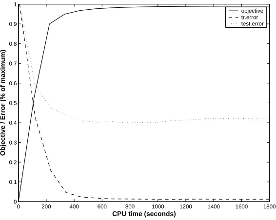
[image:20.612.165.448.92.318.2]

objective tr.error test.error

Figure 2: The objective function (% of optimum) andℓ_∆ losses forH-M3on training and test sets (WIPO-alpha)

likelihood

u(x) =argmax_y∈YTP(y|x) =argmaxyw

T_φ(x,y),

where

Y

T is the set of multilabels that correspond to unions of partial paths in T . The algorithm is otherwise the same as the one in 3.4, but the inconsistent edge-labelings are not taken into account in the maximization.

Efficiency of optimization. To give an indication of the efficiency of theH-M3algorithm, Figure 2 shows an example learning curve on WIPO-alpha dataset. The number of dual variables for this training set is just over one million with a joint kernel matrix with approx 5 billion entries. Note that the solutions for this optimization are not sparse, typically less than 25% of the marginal dual variables are zero. Training and test losses (ℓ_∆) are all close to their optima within 10 minutes of starting the training, and the objective is within 2 percent of the optimum in 30 minutes.

To put these results in perspective, for the WIPO data setSVM(SVM-light) takes approximately 50 seconds per node, resulting in a total running time of about 2.5 hours, which makes it significantly slower thanH-M3, in these tests. It is possible that using early stopping forSVMthe training time

100 1000 10000 4000

4500 5000 5500 6000 6500 7000

CPU time (seconds)

Objective

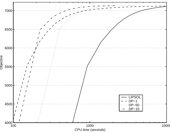
[image:21.612.165.446.89.308.2]

LIPSOL DP−1 DP−50 DP−10

Figure 3: Learning curves for H-M3 using LIPSOL and dynamic programming (DP) to compute update directions (WIPO-alpha). Curves with iteration limits 1,10 and 50 are shown for DP. The LIPSOL curve is computed with iteration limit set to 1.

The running time of H-RLSwas slower than the other methods, however this could be due to

our unoptimized implementation. It is our expectation that it would be very close to the time taken byH-SVMif coded more efficiently.

Therefore, the methods presented in this paper are very competitive from a computational ef-ficiency point of view to other methods which do not operate in the large feature/output spaces of

H-M3.

Figure 3 shows on WIPO-alpha the efficiency of the dynamic programming (DP) based com-putation of update directions as compared to solving the update directions with MATLAB’s linear interior point solver LIPSOL. The DP based updates result in an order of magnitude faster optimiza-tion than using LIPSOL.

In addition for DP the effect of the iteration limit for optimization speed is depicted. Setting the iteration limit too low (1) or too high (50) slows down the optimization, for different reasons. A too tight iteration limit makes the overhead in moving from one example to the other dominate the running time. A too high iteration limit makes the the algorithm spend too much time optimizing the dual variables of a single example. Unfortunately, it is not straightforward to suggest a iteration limit that would be universally the best, as the optimal value depends on the dataset.

Test loss

ℓ0/1 ℓ∆ ℓH˜ +scaling

Tr. loss % unif sibl. subtree ℓ∆ 27.1 0.574 0.344 0.114 0.118 ℓ_H˜-unif 26.8 0.590 0.338 0.118 0.122

ℓH˜-sibl. 28.2 0.608 0.381 0.109 0.114

ℓH˜-subtree 27.9 0.588 0.373 0.109 0.109

ℓ0/1 ℓ∆ ℓH˜ +scaling

Tr. loss % unif sibl. subtree ℓ∆ 70.9 1.670 0.891 0.050 0.070 ℓH˜-unif. 70.1 1.721 0.888 0.052 0.074

ℓH˜-sibl. 64.8 1.729 0.927 0.048 0.071

[image:22.612.192.422.88.250.2]

ℓ_H˜-subtree 65.0 1.709 0.919 0.048 0.072

Table 1: Prediction losses obtained using different training losses on Reuter’s (top) and WIPO-alpha data (bottom). The lossℓ0/1 is given as a percentage, the other losses as averages

per-example.

ℓH˜-subtree) may lead to a reduced 0/1 loss on the test set. On Reuters dataset this effect is not

observed, however this is due to the fact that the label tree of the Reuters data set is very shallow.

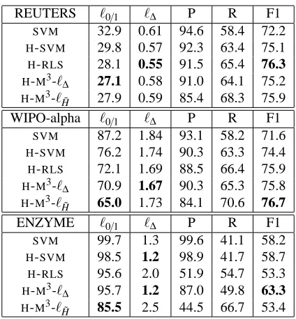
Comparison of predictive accuracies of different algorithms. In our final test we compare the predictive accuracy ofH-M3to other learning methods. ForH-M3we include the results for training

withℓ∆andℓ_H˜-subtree losses. For trainingSVMandH-SVM, these losses produce the same learned model.

Table 2 depicts the different test losses, as well as the standard information retrieval statistics precision (P), recall (R) and F1 statistic (F1=2PR/(P+R)). Precision and recall were computed over all microlabel predictions in the test set. FlatSVMis expectedly inferior to the competing

algo-rithms with respect to most statistics, as it cannot utilize the dependencies between the microlabels in any way. The two variants ofH-M3are the most efficient in getting the complete tree correct as shown by the lower zero-one loss. With respect to other statistics, the hierarchical methods are quite evenly matched overall.

Finally, to highlight the differences between the predicted labelings, we computed level-wise precision and recall values, that is, the set of predictions contained all test instances and microlabels on a given level of the tree (Table 3). On all datasets, recall of all methods, especially withSVMand H-SVM, diminishes when going farther from the root. H-M3is the most efficient method in fighting the recall decline, and is still able to obtain reasonable precision on REUTERS and WIPO-alpha, especially when trained with the hierarchical loss.

REUTERS ℓ0/1 ℓ∆ P R F1 SVM 32.9 0.61 94.6 58.4 72.2

H-SVM 29.8 0.57 92.3 63.4 75.1

H-RLS 28.1 0.55 91.5 65.4 76.3

H-M3-ℓ∆ 27.1 0.58 91.0 64.1 75.2

H-M3-ℓH˜ 27.9 0.59 85.4 68.3 75.9

WIPO-alpha ℓ0/1 ℓ∆ P R F1 SVM 87.2 1.84 93.1 58.2 71.6

H-SVM 76.2 1.74 90.3 63.3 74.4

H-RLS 72.1 1.69 88.5 66.4 75.9

H-M3-ℓ∆ 70.9 1.67 90.3 65.3 75.8

H-M3-ℓH˜ 65.0 1.73 84.1 70.6 76.7

ENZYME ℓ0/1 ℓ∆ P R F1 SVM 99.7 1.3 99.6 41.1 58.2

H-SVM 98.5 1.2 98.9 41.7 58.7 H-RLS 95.6 2.0 51.9 54.7 53.3

H-M3-ℓ∆ 95.7 1.2 87.0 49.8 63.3

[image:23.612.200.412.87.316.2]

H-M3-ℓH˜ 85.5 2.5 44.5 66.7 53.4

Table 2: Prediction lossesℓ_0/1andℓ_∆, precision, recall and F1 values obtained using different learn-ing algorithms. All figures are given as percentages. Precision and recall are computed in terms of totals of microlabel predictions in the test set.

6. Conclusions and Future Work

In this paper we have proposed a new method for training variants of the Maximum Margin Markov Network framework for hierarchical multi-category text classification models.

Our method relies on a decomposition of the problem into single-example sub problems and conditional gradient ascent for optimisation of the subproblems. The method scales well to medium-sized datasets with label matrix (examples × microlabels) size upto hundreds of thousands, and via kernelization, very large feature vectors for the examples can be used. Experimental results on three classification tasks show that using the hierarchical structure of multi-category labelings leads to improved performance over the more traditional approach of combining individual binary classifiers.

REUTERS Level 0 Level 1 Level 2 Level 3

SVM 92.4/89.4/90.9 96.8/38.7/55.3 98.1/49.3/65.6 81.8/46.2/59.0

H-SVM 92.4/89.4/90.9 93.7/43.6/59.5 91.1/61.5/73,4 72.0/46.2/56,3

H-RLS 93.2/89.1/91.1 90.9/46.8/61.8 89.7/64.8/75.2 76.0/48.7/59.4

H-M3-ℓ∆ 94.1/83.0/88.2 87.3/48.9/62.7 91.1/63.2/74.6 79.4/69.2/73.9

H-M3-ℓ_H˜ 91.1/87.8/89.4 79.2/53.1/63.6 85.4/66.6/74.8 77.9/76.9/77.4

WIPO-alpha Level 0 Level 1 Level 2 Level 3

SVM 100/100/100 92.1/77.7/84.3 84.4/42.5/56.5 82.1/12.8/22.1

H-SVM 100/100/100 92.1/77.7/84.3 79.6/51.1/62.2 77.0/24.3/36.9

H-RLS 100/100/100 91.3/79.1/84.8 78.2/57.0/65.9 72.6/29.6/42.1

H-M3-ℓ∆ 100/100/100 90.8/80.2/85.2 86.1/50.0/63.3 72.1/31.0/43.4

H-M3-ℓH˜ 100/100/100 90.9/80.4/85.3 76.4/62.3/68.6 60.4/39.7/47.9

ENZYME Level 0 Level 1 Level 2 Level 3

SVM 100/100/100 84.3/4.9/9.3 100/0.4/0.8 100/0.3/0.6

H-SVM 100/100/100 84.3/4.9/9.3 72.3/1.9/3.7 67.5/1.5/2.9

H-RLS 100/97.4/98.7 33.0/39.3/35.9 22.4/22.6/22.5 15.2/17.0/16.0

H-M3-ℓ∆ 100/100/100 61.2/30.8/41.0 49.8/13.3/21.0 52.9/4.7/8.6

[image:24.612.135.479.88.313.2]

H-M3-ℓH˜ 100/100/100 49.3/56.0/52.4 21.5/42.5/28.6 14.7/35.2/20.7

Table 3: Precision/Recall/F1 statistics for each level of the hierarchy for different algorithms on Reuters RCV1 (top), WIPO-alpha (middle), and ENZYME datasets (bottom).

Acknowledgments

References

S. M. Aji and R. McEliece. The generalized distributive law. IEEE Transactions on Information

Theory, 46(2):325–343, 2000.

Y. Altun, I. Tsochantaridis, and T. Hofmann. Hidden markov support vector machines. In

Interna-tional Conference of Machine Learning, 2003.

D. Bertsekas. Nonlinear Programming. Athena Scientific, 1999.

L. Cai and T. Hofmann. Hierarchical document categorization with support vector machines. In 13

ACM CIKM, 2004.

N. Cancedda, E. Gaussier, C. Goutte, and J.-M. Renders. Word-sequence kernels. Journal of

Machine Learning Research, 3:1059–1082, 2003.

N. Cesa-Bianchi, C. Gentile, A. Tironi, and L. Zaniboni. Incremental algorithms for hierarchical classification. In Neural Information Processing Systems, 2004.

N. Cristianini and J. Shawe-Taylor. An Introduction to Support Vector Machines. Cambridge Uni-versity Press, 2000.

O. Dekel, J. Keshet, and Y. Singer. Large margin hierarchical classification. In ICML’04, pages 209–216, 2004.

S. T. Dumais and H. Chen. Hierarchical classification of web content. In SIGIR’00, pages 256–263, 2000.

T. Gartner. A survey of kernels for structured data. ACM SIGKDD Explorations, pages 49–58, 2003.

T. Hofmann, L. Cai., and M. Ciaramita. Learning with taxonomies: Classifying documents and words. In NIPS Workshop on Syntax, Semantics, and Statistics, 2003.

T. Joachims. Text categorization with support vector machines: Learning with many relevant fea-tures. In Proceedings of the European Conference on Machine Learning, pages 137 – 142, Berlin, 1998. Springer.

D. Koller and M. Sahami. Hierarchically classifying documents using very few words. In ICML’97, pages 170–178, 1997.

F. Kschischang, B. Frey, and H.-A. Loeliger. Factor graphs and the sum-product algorithm. IEEE

Transactions on Information Theory, 47:498–519, 2001.

J. Lafferty, X. Zhu, and Y. Liu. Kernel conditional random fields: representation and clique selec-tion. In Proc. 21th International Conference on Machine Learning, pages 504–511, 2004.

C. Leslie, E. Eskin, and W. S. Noble. The spectrum kernel: A string kernel for SVM protein classification. In Proceedings of the Pacific Symposium on Biocomputing, pages 564 – 575, 2002.