On the equivalence between total least squares and
maximum likelihood PCA
M. Schuermans
a,∗, I. Markovsky
a, Peter D. Wentzell
b, S. Van Huffel
aaKULeuven, ESAT-SCD, Kasteelpark Arenberg 10, B-3001 Leuven-Heverlee, Belgium
bTrace Analysis Research Centre, Department of Chemistry, Dalhousie University, Halifax, NS, Canada B3H 4J3
Available online 26 January 2005
Abstract
The maximum likelihood PCA (MLPCA) method has been devised in chemometrics as a generalization of the well-known PCA method in order to derive consistent estimators in the presence of errors with known error distribution. For similar reasons, the total least squares (TLS) method has been generalized in the field of computational mathematics and engineering to maintain consistency of the parameter estimates in linear models with measurement errors of known distribution. The basic motivation for TLS is the following. Let a set of multidimensional data points (vectors) be given. How can one obtain a linear model that explains these data? The idea is to modify all data points in such a way that some norm of the modification is minimized subject to the constraint that the modified vectors satisfy a linear relation. Although the name “total least squares” appeared in the literature only 25 years ago, this method of fitting is certainly not new and has a long history in the statistical literature, where the method is known as “orthogonal regression”, “errors-in-variables regression” or “measurement error modeling”. The purpose of this paper is to explore the tight equivalences between MLPCA and element-wise weighted TLS (EW-TLS). Despite their seemingly different problem formulation, it is shown that both methods can be reduced to the same mathematical kernel problem, i.e. finding the closest (in a certain sense) weighted low rank matrix approximation where the weight is derived from the distribution of the errors in the data. Different solution approaches, as used in MLPCA and EW-TLS, are discussed. In particular, we will discuss the weighted low rank approximation (WLRA), the MLPCA, the EW-TLS and the generalized TLS (GTLS) problems. These four approaches tackle an equivalent weighted low rank approximation problem, but different algorithms are used to come up with the best approximation matrix. We will compare their computation times on chemical data and discuss their convergence behavior.
© 2004 Elsevier B.V. All rights reserved.
Keywords: TLS; MLPCA; Rank reduction; Measurement errors
1. Introduction
1.1. Total least squares: problem formulation, algorithms and extensions
The total least squares (TLS) method is one of several lin-ear parameter estimation techniques that has been devised to compensate for data errors. The univariate line fitting prob-lem was already discussed since 1877[1]. More recently, the TLS approach to fitting has also stimulated interests outside statistics. One of the main reasons for its popularity is the
∗Corresponding author. Tel.: +32-16321143.
E-mail address: [email protected] (M. Schuermans).
availability of efficient and numerically robust algorithms in which the singular value decomposition (SVD) plays a promi-nent role[2]. Another reason is the fact that TLS is an applica-tion oriented procedure. It is suited for situaapplica-tions in which all data are corrupted by noise, which is almost always the case in engineering applications. In this sense, TLS and errors-in-variables (EIV) modeling are a powerful extension of classi-cal least squares and ordinary regression, which corresponds only to a partial modification of the data. A comprehensive de-scription of the state of the art on TLS from its conception up to the summer of 1990 and its use in parameter estimation has been presented in[3]. While the latter book is entirely devoted to TLS, a second[4]and third book[5]present the progress in TLS and in the broader field of errors-in-variables modeling respectively from 1990 till 1996 and from 1996 till 2001.
The problem of linear parameter estimation arises in a broad class of scientific disciplines such as signal processing, automatic control, system theory and in general engineering, statistics, physics, economics, biology, medicine, etc. It starts from a model described by a linear equation:
ξ1b1+ · · · +ξnbn=η (1)
where ξ1, . . . , ξn and η denote the variables and b= [b1, . . . , bn]∈Rnplays the role of a parameter vector that characterizes the specific system. A basic problem of applied mathematics is to determine an estimate of the true but
un-known parameters from given measurements of the variables.
In general,ηcan be a vector of dimensiond >1. In this case, the parameters form a matrix B and more than one (indepen-dent) linear relationship betweenηand the variablesξi has to be estimated. This gives rise to an overdetermined set of
m linear equations (m > n):
XB≈Y (2)
where the ith row of data matrixX∈Rm×nand vectorY ∈
Rm×dcontain respectively the measurements of the variables ξ1, . . . , ξnandη.
In the classical least squares approach, as commonly used in ordinary regression, the measurements X of the variables
ξi are assumed to be free of error and hence, all errors are confined to the observations Y. However, this assumption is frequently unrealistic: sampling errors, human errors, mod-eling errors and instrument errors may imply inaccuracies of the data matrix X as well. One way to take errors in X into account is to introduce perturbations also in X. Therefore, the following TLS problem was introduced in the field of computational mathematics[2,6](R(X) denotes the range of
X and X Fits Frobenius norm[7]):
Definition 1 (Total least squares problem). Given an
overde-termined set of m linear equations XB≈Y in n×d un-knowns B. The total least squares problem seeks to
min
X,Y,Bˆ
[XY] Fsubject to (X−X) ˆB=Y−Y
(3) ˆ
Bis called a TLS solution and [XY] the corresponding TLS correction.
In most multivariate problems, the TLS problem(3)has a unique solution which can be obtained from a simple scal-ing of the d right sscal-ingular vectors of [X Y] corresponding to its d smallest singular values. Extensions of this basic TLS problem to problems in which the TLS solution is no longer unique (called minimum norm TLS since then the solution with minimal norm is selected) or fails to have a solution altogether (called non-generic TLS) and to mixed LS-TLS problems that assume some of the columns of X to be error-free, are considered in detail in[3]. In addition, it is shown how to speed up the TLS computations directly by computing
the SVD only partially or iteratively if a good starting vector is available. More recent advances, e.g. recursive TLS al-gorithms, neural based TLS alal-gorithms, rank-revealing TLS algorithms, regularized TLS algorithms, TLS algorithms for large scale problems, etc., are reviewed in[4,5].
Under specific conditions, the TLS solution, as introduced in numerical analysis, computes optimal parameter estimates in models with only measurement error, referred to as clas-sical EIV models. These models are characterized by the fact that the true values of the observed variables satisfy one or more unknown but exact linear relations of the form(1). In particular, we define[8–10]the following.
Definition 2 (Multivariate EIV regression model). Assume
that the m measurements in X, Y are related to n×d un-knowns B by:
ΞB=η, X=Ξ+XandY =η+Y (4)
whereX, Yrepresent the measurement errors and all rows of [X Y] are i.i.d. with zero mean and covariance matrix
C, known up to a scalar multipleσν2.
If additionallyC=σν2I is assumed with I the identity ma-trix (i.e. xij andyij are uncorrelated random variables with equal variance) and limm→∞m1ΞΞexists and is pos-itive definite, then it can be proven [9,6]that the TLS so-lution ˆBofXB≈Y estimates the true parameter values B, given by (ΞΞ)−1Ξη, consistently, i.e. ˆBconverges to B as
m→ ∞. This TLS property does not depend on any assumed distributional form of the errors. If additionally the errors are normal, then TLS computes the ML estimate. It should be noted that the TLS correction [XY], being of rank≤d, cannot be considered as an appropriate estimator for the true measurement errors X andY, added to the data [2,3]. Note also that the LS estimates are inconsistent in this case. In these cases, TLS gives better estimates than does LS, as confirmed by simulations [3]. This situation may occur far more often in practice than is recognized. It is very common in agricultural, medical and economic science, in humanities, business and many other data analysis situations. Hence TLS should be a quite useful tool to data analysts. In fact, the key role and importance of LS in regression analysis is the same as that of TLS in EIV regression. Nevertheless, a lot of con-fusion exists in the fields of numerical analysis and statistics about the principle of TLS and its relation to EIV modeling. Roughly speaking, TLS is a special case of EIV estimation and, as such, TLS is reduced to a method in statistics but, on the other hand, TLS appears in many other fields, where mainly the data modification idea is used and explained from a geometric point of view, independently from its statistical interpretation.
covari-ance matrix, equal to the identity matrix up to an unknown scalar. Most published TLS algorithms just handle this case while other more useful EIV regression estimators did not receive enough attention in computational mathematics. To relax these restrictions, several extensions of the TLS prob-lem have been investigated. In particular, the mixed LS-TLS problem formulation allows extension of the consistency of the TLS estimator in EIV models, where some of the variables
ξi are measured without error. The data least squares prob-lem refers to the special case in which all variables except
ηare measured with error and was introduced in the field of signal processing by DeGroat and Dowling[11]in the mid-1990s. Whenever the errors are independent but unequally sized, weighted TLS problems should be considered using appropriate diagonal scaling matrices in order to maintain consistency. If, additionally, the errors are also correlated, then the generalized TLS (GTLS)[12]problem formulation (defined in the next section) allows extension of the con-sistency of the TLS estimator in EIV models, provided the corresponding error covariance matrix Cis known up to a factor of proportionality (seeDefinition 2).
More general problem formulations, such as restricted
TLS, which also allow the incorporation of equality
con-straints, have been proposed, as well as equivalent problem formulations using other Lp norms and resulting in the
so-called Total Lpapproximations (see[3]for references). The latter problems proved to be useful in the presence of out-liers. Robustness of the TLS solution is also improved by adding regularization, resulting in the regularized TLS meth-ods[5,13,14]. In addition, various types of bounded uncer-tainties have been proposed in order to improve robustness of the estimators under various noise conditions and algorithms are outlined[4,5].
Furthermore, constrained TLS problems have been for-mulated. Arun[15]addressed the unitarily constrained TLS problem, i.e.,XB≈Y, subject to the constraint that the solu-tion matrix B should be unitary. He proved that this solusolu-tion is the same as the solution to the orthogonal Procrustes prob-lem[7, p. 582]. Abatzoglou et al.[16]considered yet another constrained TLS problem, which extends the classical TLS problem(3) to the case where the errors [X Y] in the data [X Y] are algebraically related. However, if there is a linear dependence among the error entries in [X Y], then the TLS solution no longer has optimal statistical prop-erties (e.g. maximum likelihood in case of normality). This happens, for instance, in dynamic system modeling when we try to estimate the impulse response of a system from its input and output by discrete deconvolution. In these so-called structured TLS problems, the data matrix [X Y] is structured, typically block Toeplitz or Hankel. In order to preserve maximum likelihood properties and consistency of the solution[16,17], the TLS problem formulation, given in
Definition 1, must be extended with the additional constraint that any (affine) structure of X or [X Y] must be preserved inXor [XY], whereXandYare chosen to min-imize the error in the discrete L1, L2and L∞norm. For L2
norm minimization, various computational algorithms have been presented, as surveyed in[4,5], and shown to reduce the computation time by exploiting the matrix structure in the computations. In addition, it is shown how to extend the problem and solve it, if latency or equation errors are in-cluded. Recently, robustness of the structured TLS solution has been improved by adding regularization, see e.g.[18].
Yet, another important extension is the element-wise
weighted TLS (EW-TLS) estimator[19,20] (see definition in the next section). EW-TLS computes consistent estimates in linear EIV models, where the measurement errors are element-wise differently sized or, more generally, where the corresponding error covariance matrices may differ from row to row, provided the total covariance structure of the errors is known up to a scalar factor. Some of the variables are allowed to be exactly known (observable)[5,21]. Mild con-ditions for weak consistency of the EW-TLS estimator have been given and an iterative procedure to compute it has been proposed.
1.2. Total least squares in chemometrics: state-of-the-art
Although TLS has already been applied in chemometrics since 1984[22], its concept and properties are not well known in chemometrics and in fact a lot of confusion exists about its proper use and relation to well-known chemometric tech-niques such as principal component analysis (PCA), partial least squares (PLS) and other EIV approaches such as latent root regression (LRR).
Several authors, such as Burnham et al. [23], de Jong
[24,25]and Phatak[4,26,27], have described the close re-lationships between a variety of multivariate regression tech-niques, including TLS, mainly from a theoretical point of view. Although TLS should be primarily used for parameter estimation, it can be used for prediction provided the solu-tion is appropriately computed[22,28]. In[22], the prediction accuracy and stability of the TLS estimator is compared to that of ordinary LS, PC regression (PCR), ridge regression and shrunken estimators in a chemical example in multivari-ate regression in the presence of multicollinearities among the independent variables. In many chemical applications of multivariate regression like the present example of relation-ships between chemical structure and biological activity, the predictive properties of the model are of prime importance and the regression estimates therefore often need to be sta-bilized. The example[22]shows that minimum norm TLS gives a solution to the multivariate regression problem which is stabilized in comparison with the LS solution and which has (at least in the example investigated) minimal predic-tion error. Stabilizapredic-tion is performed by reducing the matrix [X y] to a matrix of much smaller rank.
More generally, the usefulness of an EIV model for pro-viding insights into the multivariate calibration problem[29]
framework with maximum likelihood properties. Moreover, using the responses (spectra) from the available members of the prediction set together improves the accuracy of the new concentrations compared to estimation based on only one re-sponse of the current member of the prediction set.
Another EIV approach to multivariate calibration and mul-tivariate regression, two kernel problems in analytical chem-istry, was developed by Wentzell et al.[28], who general-ized the PCA method to maximum likelihood PCA (MLPCA)
[31,32]. MLPCA is an analog to PCA that incorporates in-formation about measurement errors to develop PCA models that are optimal in a maximum likelihood sense. A glob-ally convergent algorithm based on an alternating regression method has been derived. Generalization of the algorithm al-lows its adaptation to cases of correlated errors provided the error covariance matrix is known. Simplifications to the orig-inal algorithm apply when errors are correlated only within the rows of a data matrix and when all of these row covari-ance matrices are equal. Simulated and experimental data for three-component mixtures show that inclusion of error co-variance information via MLPCA outperforms PCA when the true error covariance matrix is available. Using MLPCA, two approaches to multivariate calibration have been described that allow information on measurement uncertainties to be included in the calibration process in a statistically meaning-ful way. These methods, referred to as maximum likelihood PCR (MLPCR) and maximum likelihood LRR (MLLRR) are based on principles of ML parameter estimation and general-ize PCR, which has been widely used in chemistry, and LRR
[33,34], which has been almost ignored in this field. Whereas MLPCR is based on the decomposition of the calibration matrix X by MLPCA, MLLRR decomposes the augmented data matrix [X Y] using MLPCA. In multivariate calibra-tion, this is the original calibration matrix of response vari-ables X augmented by the corresponding concentration vec-tors Y. (ML)LRR is equivalent to (EW)TLS in the sense that it computes the best lower rank approximationD =[ ˆXYˆ] of the augmented data matrixD=[X Y] in a (weighted) least squares sense. If ˆX∈R( ˆY), TLS computes the minimum norm solution which equals the minimum norm LS solution and hence TLS is equivalent to LRR, as reported in[28]. How-ever, if only non-predictive multicollinearities (i.e. linear de-pendencies among the columns of X only) have been removed via the rank reduction, then ˆX /∈R( ˆY) and the TLS problem is called non-generic. In this case, the LRR solution differs from the non-generic TLS solution, as shown in[3]. After removing the non-predictive multicollinearities, the LRR es-timate is found by minimizing a sum of squared residuals, while the non-generic TLS solution is found by minimizing the corrections applied to the data such that the corrected data satisfy the constraint ˆX∈R( ˆY). By using estimates of the measurement error variance, MLPCR and MLLRR are able to extract the optimum amount of information from each mea-surement and, thereby, outperform conventional multivariate calibration methods such as PCR and PLS when there is non-uniform error structure. Using simulated and experimental
data of three-component mixtures, it is shown that the ML methods outperform PCR and PLS in case of non-uniform er-rors. MLLRR generally performed better than MLPCR, but in most cases the improvement was marginal.
Finally, it should be noted that structured TLS (STLS) clearly differs from dynamic PCA[35]. Although both meth-ods focus on modeling dynamic systems in an EIV context, dynamic PCA is based on computing the truncated SVD of an input/output data matrix and as such does not preserve the matrix structure during rank reduction in contrast with STLS and is hence not optimal.
1.3. The use of TLS and extensions in multivariate (ML)PCR
From the previous subsections it should be clear that TLS and its extensions can be used in any multivariate (ML) re-gression/calibration problemXB≈Yby computing the best lower rank approximation ˆD=[ ˆXYˆ] of the augmented data matrixD=[X Y] according to a weighted norm. As such, (EW)TLS is equivalent to (ML)LRR in problem formula-tion. However, (EW)TLS can also be used in any multi-variate (ML)PCR problem XB≈Y where an MLPCA of
X is sought prior to the computation of B. Indeed, assume
that the true pseudorank of X is p and the measurement er-rors on the elements of X are i.i.d. normal, then the opti-mal rank p matrix approximation ˆX∈Rm×Nin an ML sense is obtained by solving the TLS problem X1B≈X2 where
X is split up in two parts X=[X1X2] such that X1 has
p columns and rank p. The TLS approach then computes
minimal (with respect to the Frobenius norm) corrections
X=[X1−X1ˆ X2−X2ˆ ] such that ˆX=[ ˆX1X2ˆ ] is of rank p. In other words, TLS projects the dataXinto a lower di-mensional (of dimension p) subspaceR( ˆX) such that exactly
N−pindependent linear relations are imposed between ˆX1 and ˆX2. Equivalently, for correlated normally distributed er-rors where the error covariance matrix Wi of the errors in each row of the data matrix X is known, an optimal lower rank approximation in an ML sense is obtained by minimiz-ing a weighted sum of squared corrections. If allWiare equal to each other, EW-TLS reduces to GTLS. As such, TLS and EW-TLS algorithms can be applied to compute the PCA and MLPCA of a matrix D=X, as used in PCR and MLPCR, orD=[X Y], as used in LRR and MLLRR. Other methods exist in the literature to tackle the weighted low rank matrix approximation problem, such as the weighted low rank ap-proximation (WLRA) method[36]. It is the goal of this paper to compare the performance of the algorithms used for solv-ing TLS problems and its extensions with the algorithms used in chemometrics for computing PCA and MLPCA. Also, the WLRA algorithm will be considered in this comparison.
matrix ˆDof a given data matrix D. InSection 4we will com-pare their computation times on simulated as well as real-life chemical data and discuss their convergence behavior. Con-clusions are made inSection 5.
2. Weighted low rank matrix approximation: problem formulation
When the measurement noise is centered, normal and in-dependent identically distributed, the optimal closeness norm is the Frobenius norm, · F. This is used in the well-known TLS and the PCA methods. Nevertheless, when the measure-ment errors are not identically distributed the Frobenius norm is no longer optimal and a weighted norm is needed instead. The weighting is related to the noise covariance matrix. In this case a closed-form solution is no longer available and is only implicitly defined via a non-convex optimization prob-lem, which is the case in this paper.
Mathematically, we will consider the following weighted low rank matrix approximation problem:
min
ˆ D vec
(D−Dˆ)W−1vec(D−Dˆ) s.t.rank( ˆD)≤p (5)
with D∈Rm×N, m≤N, the noisy data matrix, p < m,
D=D−Dˆ the estimated measurement noise and W the covariance matrix of vec(D) where vec(D) stands for the vectorized form ofD, i.e., a vector constructed by stacking the consecutive columns ofDin one vector.
We will discuss the WLRA, the MLPCA, the EW-TLS and the GTLS method to tackle this matrix weighted low rank ap-proximation problem. These methods differ in the representa-tion of the rank constraint rank( ˆD)≤pin problem(5)and in the applied optimization technique in order to solve problem
(5). In this section a short description is given of the different problem formulations and the different approaches for these methods. In the next section their different algorithms will be discussed.
The different representations of the rank constraint are the following:
C1: ˆD=TP, whereT ∈Rm×pandP ∈RN×p;
C2: ˆDN=0, whereN∈RN×(N−p)andNN=I;
C3: ˆD
B −IN−p
=0, whereB∈Rp×(N−p).
C1 and C2 are equivalent. RepresentationsC2 andC3 only differ in the wayNis restricted to be full rank. Represen-tationC2 imposes the additional constraintNN=I, while representationC3 sets the lower (N−p)×(N−p) block of
Nto−I. The constraintNN=Ihas the advantage that it avoids the so-called non-generic cases, but it is more difficult to deal with. Indeed, by usingC3 for representing the rank constraint, the condensed problem is an unconstrained op-timization problem, while usingC2 the condensed problem remains to a constrained optimization problem since the con-straintNN=Icannot be substituted in the object function.
Any of the representationsC1 –C3 for the rank constraint is bilinear. To handle such a bilinear problem, different opti-mization techniques can be used:
T1: applying an alternating least squares algorithm;
T2: eliminating one of the variables and obtaining an equiv-alent problem in the other variable;
T3: linearizing the constraint and solving iteratively equality-constrained least squares problems.
Now, we can formulate the WLRA[36], the MLPCA[31], the EW-TLS[19]and the GTLS[12]problem:
WLRA : min
D,Nvec(D)W−1vec(D) s.t.
(D−D)N=0, whereN∈RN×(m−p)and
NN=I.
MLPCA : minT,Pvec(D)W−1vec(D) s.t.
D=D−TP, withT ∈Rm×pandP ∈RN×p.
EW-TLS : minB,ˆDmi=1vec(Di)Wi−1vec(Di) s.t. (D−D)
ˆ
B −I
=0 withDi ∈RNthe ith row of
D andWi the ith weighting matrix defined as the covariance matrix of the errors in the ith row of the data matrix D.
GTLS : minB,ˆ D2 mi=1vec(D2 ,i)Wf−1vec(D2 ,i) s.t. (D−D)
ˆ
B −I
=0 withD2 ,i∈RN2 the ith row
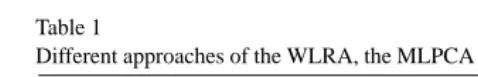
Table 1
Different approaches of the WLRA, the MLPCA and the EW-TLS problem
Approach WLRA MLPCA EW-TLS
Rank constraint C2 C1 C3
Optimization technique T2 T1 T2
Another difference between the WLRA-/MLPCA prob-lem and the two TLS probprob-lem formulations is the mation variable. The first two problems are matrix approxi-mation problems to find the approxiapproxi-mation matrix ˆD, while the latter ones are looking for a solution ˆBof a linear model. Nevertheless, one can easily find the corresponding ˆBfrom
ˆ
Dsuch that ˆD
ˆ
B −I
=0 and at any optimal solution ˆB,Dˆ
from the TLS problem formulations ˆDcan be obtained from ˆ
Band the weighting matrices via a closed form expression
[20, Eq. (14)]. Thus except for the above-mentioned differ-ences, the four formulated problems are equivalent. Their numerical algorithms, however, are different. This will be discussed in the next section.
InTable 1the rank constraint representations and the op-timization approaches of the four mentioned problems are summarized. Because the GTLS problem is a special case of the EW-TLS problem withWi=Wf fori=1, . . . , m, the GTLS problem is not included in the table.Fig. 3explains the hierarchy of the four problem formulations.
3. Different algorithms for one problem
3.1. GTLS algorithm
The GTLS algorithm is derived for the special case when
W=blkdiag(Wf, . . . , Wf) withWf ∈RN×N.
The following input/output representation of the model is used:
rank( ˆD)≤p⇐⇒XˆBˆ =Y,ˆ where ˆD=[ ˆXYˆ]
with col dim( ˆX)=p,Xˆ ∈Rm×p and Yˆ ∈Rm×(N−p). Hence, the low rank approximation problem(5)can be writ-ten as
min
ˆ B,D
m
i=1
vec(Di)Wf−1vec(Di) s.t.(D−D)
B −I
=0
(6) To compute a solution of problem(6)the data matrixD= [X Y] is scaled such that the error covariance matrixWf∗of the transformed dataD∗=[X∗Y∗] is diagonal with equal variances, i.e. Wf∗∼I. The classical TLS algorithm[3] is used to solve this transformed set of equationsX∗B∗≈Y∗ and finally the solution of the transformed set is converted into
a solution of the original set of equationsXB≈Y. An outline of the GTLS algorithm is given inAlgorithm 1. Alternatively, the GTLS problem can also be solved by making use of the Generalized SVD[7]. This approach is recommended when
Wfis close to rank deficiency. For more details, the interested reader is referred to[12].
Algorithm 1. GTLS algorithm via rescaling the data.
1. Input: the data matrix D∈Rm×N, the error covariance matrixWf ∈RN×Nwhich is equal for all rows of D and a rank specification p.
2. DefineD=[X Y], withX∈Rm×pandY ∈Rm×(N−p). 3. Compute the Cholesky factorization ofWf :Wf =CC. 4. Rescale the data matrix D:
D∗ =[X∗ Y∗]=[X Y]C−1
=[X Y]
p N−p
C11
0
C12 C22
p N−p
5. Apply the classical TLS algorithm to the dataD∗: compute a rank p truncated SVD approximationD∗tls=UpSpVp
of D∗, with the SVD of the matrixD∗ equal toUSV,
Up the truncation of the matrix U to m×p, Sp the truncation of S to p×p and Vp the truncation of V toN×p, UpUp=I, VpVp=I; compute the solution
B∗tlsofX∗B∗≈Y∗:
ifp≥N−pthenB∗tls= −V12V22−1,where p N−p
V11 V21
V12 V22
p N−p
elseB∗tls=(V11)−1V21.
6. Output: ˆBgtls=(C11B∗tls−C12)C−221; ˆDgtls =D∗tlsC.
Note 1 (Special cases: ordinary TLS and weighted TLS).
It is worth noting that when W∼I (i.e., the errors of the data matrix D are uncorrelated and equally sized), the GTLS solution reduces to the ordinary TLS estimate. Whenever the errors are uncorrelated but unequally sized (W is diagonal), the GTLS problem formulation reduces to the weighted TLS problem.
3.2. Alternating least squares algorithm
The alternating least squares algorithm is based on an im-age representation of the model
rank( ˆD)≤p⇐⇒Dˆ =TP, where
which allows us to write the low rank approximation problem
(5)equivalently as
min
T∈Rm×pP∈RminN×pvec
(D−TP)W−1vec(D−TP) (7)
The following two problems:
min
T∈Rm×pvec
(D−TP)W−1vec(D−TP) (8)
min
P∈RN×pvec
(D−TP)W−1vec(D−TP) (9)
derived from (7) by fixing, respectively, P and T to given values are least squares problems and therefore can be solved in closed form. They can be viewed as relaxations of the non-convex problem(7)to convex problems.
The alternating least squares method is an iterative method that alternately solves(8) and (9)with respectively P and T fixed to the solution of the previously solved relaxation prob-lem. The resulting alternating least squares algorithm, see
Algorithm 2, is given for the case of an arbitrary positive definite covariance matrix W. When W happens to be block diagonal or diagonal (corresponding to respectively column-wise and element-column-wise uncorrelated measurement errors),
Algorithm 2can be implemented more efficiently by taking into account the structure of W. For example, let
W =blkdiag(W1, . . . , WN), whereWi ∈Rm×m
and defineD=[d1· · ·dN]. The solution of problem(8)can be computed efficiently in this case as follows:
pi =(TWi−1T)−1TWi−1di, fori=1, . . . , N,
wherepi is the ith column ofP. In a similar (but not so straightforward) way, the block diagonal structure of W can be taken into account for improving the computational efficiency when solving problem(9). We skip the algorithmic details.
Algorithm 2. Alternating least squares algorithm.
1. Input: data matrixD∈Rm×N, covariance matrixW∈
RNm×Nm, rank specification p, and relative convergence
toleranceε.
2. Initial approximation: compute a rank p GTLS approx-imation ˆDgtlsofDwithWf = N1 Ni=1WiwhereWi is the submatrix of W at the intersection of the rows (i−1)m+1 to i·m and the columns (i−1)m+1 toi·m(see Algorithm 1 and letT(0)=Tgtlsˆ , D(0)=
ˆ
Dgtls, P(0)=Pgtlsˆ , where ˆPgtls is the matrix, such that
ˆ
Dgtls=Tgtlsˆ Pˆ
gtls.
3. k=0. 4. repeat
5. Compute the solution of(8)
vec(P(k+1))=(M(k)W−1M(k))−1M(k)W−1vec(D), where M(k)=IN⊗T(k).
6. k=k+1.
7. Compute the solution of(9)
vec(T(k+1))=(L(k)W−1L(k))−1L(k)W−1vec(D), where L(k)=P(k)⊗Id.
8. D(k)=T(k)P(k).
9. until D(k)−D(k−1) F/ D(k) F< ε. 10. Output: ˆD=D(k).
Note 2 (Initial approximation). The covariance matrix W
can partially be taken into account in the computation of the initial approximation by using the GTLS method, thereby improving the convergence rate as shown inSection 4. How-ever, the initial approximation can also be chosen to be a rank p TLS approximation ˆDtls of D, as proposed in
[31,32]: compute a rank p truncated SVD approximation
D(0)=Dtlsˆ =U
pSpVp of D, with the SVD of the matrix
D equal to USV, Up the truncation of the matrix U to
m×p, Sp the truncation of S top×p and Vp the trun-cation of V toN×p, UpUp=I, VpVp=I and let ˆTtls=
UpSp,Pˆ
tls=Vp, such that ˆDtls=Ttlsˆ Pˆtls.
The alternating least squares algorithm monotonically de-creases the cost function value, so that it is globally conver-gent. The convergence rate, however, is linear and depends on the distribution of the singular values of D[36, IV.A]. With a pair of closely spaced singular values the convergence rate could be rather low.
3.3. Algorithm of Premoli–Rastello
The algorithm of Premoli–Rastello, see[19,20]is derived for the special case when
W=blkdiag(W1, . . . , WN), whereWi∈Rm×m.
The following input/output representation of the model is used
rank( ˆD)≤p⇐⇒XˆBˆ =Y,ˆ where ˆD=[ ˆXYˆ]
with col dim( ˆX)=p,col dim( ˆY)=d, andm=p+d. The low rank approximation problem(5)can be solved partially by minimizing analytically with respect to ˆD. In this way the following equivalent unconstrained optimization problem is derived:
ˆ
B∗=arg min
ˆ
B f( ˆB), (10)
where
f( ˆB)=
N
i=1
di R(RWi−1R)−1Rdi, R=[ ˆB−I]
Define the residual matrix
E( ˆB)=(RD)=XBˆ −Y, E( ˆB)=[e1( ˆB)· · ·eN( ˆB) ]
and partitiondiandWias follows:
di =
xi yi
p
d , Wi =
p d Wx,i Wyx,i Wxy,i Wy,i p d
The first order optimality conditionf( ˆB)=0 of(10)is
2
N
i=1
(xiei ( ˆB)Γi−1( ˆB)−(Wx,iBˆ −Wxy,i)Γi−1
( ˆB)ei( ˆB)ei ( ˆB)Γi−1( ˆB))=0 where
Γi( ˆB)=RWi−1R.
We aim to find a solution off( ˆB)=0 that corresponds to a solution of the low rank approximation problem, i.e., to a global minimum point of f.
The algorithm proposed in[19]uses an iterative procedure starting from an initial approximationB(0) and generating a sequence of approximationsB(k), k=0,1,2, . . .that ap-proaches a solution off( ˆB)=0. The iteration is implicitly defined by the equation
F(B(k+1), B(k))=0, (12) where
F(B(k+1), B(k))=2
N
i=1
(xi(B(k+1)xi−yi)Γi−1(B(k))
−(Wx,iB(k+1)−Wxy,i)Γi−1(B(k))ei(B(k))ei
×(B(k))Γi−1(B(k)))
Note thatF(B(k+1), B(k)) is linear inB(k+1), so thatB(k+1) can be computed in a closed form as a function ofB(k). Eq.
(12)withB(k)fixed can be viewed as a linear relaxation of the first order optimality condition of(10), which is a highly nonlinear equation.
An outline of the Premoli–Rastello algorithm is given in
Algorithm 3. In general, solving the Eq.(12)forB(k+1) re-quires vectorization. The vec operator vectorizes a matrix column-wise and⊗denotes the Kronecker product. The fol-lowing identity is used vec(XBY)=(Y⊗X)vec(B) in or-der to transform(12) to the classical system of equations
G(B(k))vec(B(k+1))=h(B(k)), where G and h are given in the algorithm. The mappingb=vec(B)→Bis denoted by vec−1.
Algorithm 3. Algorithm of Premoli–Rastello.
1. Input: the data matrixD∈Rm×N, the covariance ma-trices {Wi}Ni=1, a rank specification p, and a conver-gence toleranceε.
2. Initial approximation: compute a GTLS solution ˆ
Bgtls of XB≈Y where D=[X Y] with Wf =
1 N
N
i=1Wi whereWiis the submatrix of W at the
in-tersection of the rows (i−1)m+1 to i·m and the columns (i−1)m+1 toi·mand letB(0)=Bgtlsˆ (see
Algorithm 1).
3. Define:D=
x1· · · y1· · ·
xN yN
p
d , whered=m−p.
4. k=0. 5. repeat
6. LetG=0pd×pdandh=0pd×1.
7. fori=1, . . . , Ndo
8. ei=B(k)xi−yi. 9. Ni=
B(k) −I
Wi
B(k) −I
−1
.
10. ni=Niei.
11. G=G+Ni⊗(xixi)−(nini )⊗Wx,i. 12. h=h+vec(xiyiNi−Wxy,inini ). 13. end for
14. Solve the systemGb=hand letB(k+1)=vec−1(b). 15. k=k+1.
16. until B(k)−B(k−1) F/ B(k) F < ε 17. Output: ˆB∗=B(k).
Note 3. In the special cases of rank reduction by one, i.e.,p=
m−1, Eq. (12)becomes particularly simple. In this case,
Γi(b(k)), ei(b(k)), andyiare scalars, so that(12)can be written as
N
i=1
(xi(xi b(k+1)−yi)Γi−1(b(k))−(Wx,ib(k+1)−Wxy,i)
Γ−1
i (b(k))ei(b(k))ei(b(k))Γi−1(b(k)))=0,
which is equivalent to a standard linear system of equations
G(b(k))b(k+1)=h(b(k)),
N
i=1
xixi
Γi(b(k))−Wx,i e2
i(b(k)) Γ2
i (b(k))
G(b(k))
bk+1
= N
i=1
xiyi
Γi(b(k))−Wxy,i e2
i(b(k)) Γ2
i (b(k))
h(b(k))
Note 4 (Relation to Gauss–Newton type algorithms).
derivation of the algorithm simpler but complicates the con-vergence analysis.
Note 5 (Convergence properties).Algorithm 3is proven to be locally convergent with a super linear convergence rate, see[20, Section 5.3]. Moreover, the convergence rate tends to quadratic as the approximation gets closer to a minimum point. The algorithm, however, is not globally convergent and simulation results suggest that the region of convergence to a minimum point could be rather small. This requires a good initial approximation for convergence.
3.4. An algorithm based on classical local optimization methods
Both the alternating least squares and the Premoli– Rastello algorithm are heuristic optimization methods. Next, we describe an algorithm for the low rank approximation problem based on classical local optimization methods. The classical local optimization methods have reached by now a high level of maturity. In particular, their convergence prop-erties are well understood, while the convergence propprop-erties of the alternative methods are still not.
In order to apply classical optimization algorithms for the solution of(5), first we have to choose a parameterization of the model. A possible parameterization is given by the in-put/output representation, so the considered problem is(10). A quasi-Newton type method requires an evaluation of the cost functionf( ˆB) and its first derivativef( ˆB). Both the cost function and its first derivative are available in closed form, so that their evaluation is a matter of numerical implementa-tion of the involved operaimplementa-tions. The computaimplementa-tional steps are summarized inAlgorithm 4. The proposed algorithm, based on a classical optimization method, is outlined inAlgorithm 5.
Algorithm 4. Cost function and first derivative evaluation.
1. Input:D∈Rm×N,{Wi}Ni=1, p, and ˆB. 2. Define:D=
x1· · · y1· · ·
xN yN
p
d , whered=m−p.
3. Letf =01×1andf=0p×d.
4. fori=1, . . . , Ndo
5. ei =Bˆxi−yi.
6. Solve the system
ˆ
B −I
WI
ˆ
B −I
ni =ei.
7. f =f+ei ni.
8. f=f+xini −(Wx,iBˆ −Wxy,i)nini . 9. end for
10. Output: the cost function f and its first derivative 2fat ˆ
B.
Algorithm 5. Algorithm based on classical local
optimiza-tion.
1. Input: the data matrixD∈Rm×N, the covariance matri-cesWi, i=1, . . . , N, a rank specification p, and a con-vergence toleranceε.
2. Initial approximation: compute a GTLS approximation ˆ
BgtlsofD, and letB(0)=Bgtls . (See Step 2 ofAlgorithm 3.)
3. Apply a standard optimization algorithm, e.g., the BFGS (Broyden, Fletcher, Goldfarb, and Shanno) quasi-Newton method, for the minimization of f over ˆBwith initial ap-proximationB(0)and with cost function and first deriva-tive evaluation performed viaAlgorithm 4. Let ˆB∗be the approximation found by the optimization algorithm upon convergence.
4. Output: ˆB∗.
The optimization problem(10)is a nonlinear least squares problem, i.e.,
f( ˆB)=F( ˆB)F( ˆB)
for certain F :Rp×d →RNd. Therefore, the use of spe-cial optimization methods like the Levenberg–Marquardt method is preferable. The vector F( ˆB), however, is com-puted numerically, so that the Jacobian J( ˆB)=δFi/δBˆj, where ˆB=vec( ˆB), cannot be found in closed form. A possi-ble workaround for this propossi-blem is proposed in[37], where an approximation, called quasi-Jacobian is used instead. The quasi-Jacobian can be evaluated in a similar way to the one for the gradient, which allows use of the Levenberg–Marquardt method for the solution of the low rank approximation prob-lem.
Note 6 (Row versus column error covariances). Algorithms 3 and 5are designed for the case whenm≥Nand row-wise correlated measurement errors. In chemometrics the data ma-trix usually has size m×N withm≤N. When the mea-surement errors are uncorrelated or column-wise correlated,
Algorithms 3 and 5can be applied to the transposed data matrix. For other cases of measurement error correlation, the algorithms need to be optimized by considering the left ker-nel of ˆD, i.e., the following modifications ofC2 andC3 should be used:
C2 :NDˆ =0, whereN∈Rm×(m−p)andNN=I;
C3 : [B−Im−p] ˆD=0, whereB∈Rp×(m−p).
4. Performance comparison of MLPCA versus EW-TLS
Mat-lab (version 6.1) on a PC i686 with 800 MHz and 256 MB memory.
The data sets which are used differ in the structure of the covariance matrix W of the measurement noise. In the first subsection we use data sets with uncorrelated measurement errors. The second subsection contains a data set with row-wise correlated measurement errors.
4.1. No correlation among the measurement errors
In this section we use data sets without any correlation among their measurement errors. For these data sets the weighting matrix W in problem(5)is diagonal.
4.1.1. Equal row error variances
In order to give results for the case of uncorrelated mea-surement noise with a diagonal covariance matrixWf which is equal for all rows, we use an experimental data set which was used previously by Wentzell and Andrews [31]. The reader is referred to the original work for a complete de-scription of the experiment. In here, we only describe shortly the experiment.
Example 1. Thirty-one three-component mixtures
contain-ing toluene, chlorobenzene and heptane were derived from an augmented, three-level, three-factor, full factorial design. The spectra were obtained over the range 400–2500 nm on an NIRSystems model 6500 grating spectrometer at intervals of 2 nm and were the average result of 32 scans. Only stan-dard deviations calculated from the replicate data for the first sample were available. The standard deviations for the first sample were used for all samples. So, the error covariance matrix was the same for every row of the measurement error matrix. Because there was no information about the correla-tions among the data, we used a diagonal covariance matrix for each row.
Because the error covariance matrix was the same for each row, the GTLS approach could be used. We applied both, the MLPCA and the GTLS, approaches to the noisy data matrix
D of size 31×1050 in order to estimate the error-free mea-surement data matrix ˆDof rank 3. The MLPCA algorithm that we used for this data set is the standard MLPCA algo-rithm for uncorrelated errors (see[31, Table 1]). The GTLS algorithm that we applied isAlgorithm 1from the previous section. For both, the MLPCA and the GTLS, algorithms the relative error D−Dˆ F
D F and the computation time is presented
[image:10.842.308.549.677.735.2]inTable 2. The table demonstrates that GTLS is a practical alternative to MLPCA for this specific class of structure in
Table 2
MLPCA and GTLS for near-infrared spectroscopic data described in Example 1
Relative error Time (s)
MLPCA 0.15834292416862 37.6150
GTLS 0.15834292417331 4.1760
the measurement error matrix. The measurement errors are uncorrelated and the covariance matrices of the errors in the rows are assumed to be equal for all rows. This class of mea-surement noise structure (uncorrelated errors with equal row error variance) is quite common for real-life data.
4.1.2. Unequal row error variances
To discuss the performance of the MLPCA and the EW-TLS approach for data with uncorrelated measurement errors, we use simulated data sets.
Example 2. The data sets all have 10 rows, but the number
of columns N increases from 10 till 200 in steps of 10. So, this simulation set contains data sets of size 10×Nand pseu-dorank 2. For each data set the error-free data matrixD0is generated by multiplying a 10×2 random matrix of full rank (with Matlab’srand) by a 2×Nmatrix that also is created withrand. The matrix of the measurement standard devia-tions corresponding to this 10×Nmatrix is determined by generating a 10×N matrix of uniform distributed random numbers between 0 and 0.01. This ensures that there is no pattern in the standard deviation matrix. Now, the 10×N matrix of measurement errorsDis generated by taking a 10×N random matrix with normally distributed elements (with Matlab’s randn) and multiplying this, element-wise, by the standard deviation matrix. Finally, the noisy data ma-trix D is the sum of the error-free mama-trixD0and the noise matrixD.
We applied the MLPCA method to the given data matrix
D and the EW-TLS method to the transposed data matrix
D (see Note 6) to approximate the ‘best’ rank 2
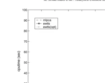
approx-imation matrix ˆD and the results are presented inTable 3
andFig. 1. For the ‘mlpca’ approach (see[31, Table 1]) the truncated SVD solution (seeNote 2) is used as initial value. For the ‘mlpca(gtls)’ approach the GTLS approximation (see
[image:10.842.42.284.698.736.2]Algorithm 1) is used as initial value instead of the truncated SVD solution.Table 3andFig. 1also contain the results of ap-plying the EW-TLS approach with two different algorithms. For ‘ewtls’Algorithm 3is used and for ‘ewtls(opt)’Algorithm 5 is applied to the transposed data. For both algorithms we have used the GTLS approximation as initial starting point.
Table 3contains the relative error D0−Dˆ F
D0 F after applying the
four algorithms to a data set of size 10×200. The results in the table are the average of the relative error over 100 rep-etitions for different noise realizations. From the table it is clear that the ‘ewtls’Algorithm 3diverges. It is very sensitive
Table 3
MLPCA and EW-TLS for data with uncorrelated measurement error de-scribed inExample 2
Approach Relative error
mlpca 0.00262998780684
mlpca(gtls) 0.00267695997595
ewtls 0.29211400246120
Fig. 1. The cputime of the MLPCA and the EW-TLS approaches for data with uncorrelated measurement error described inExample 2.
to local minima. Nevertheless, the ‘ewtls(opt)’Algorithm 5
converges to the same solution as the MLPCA algorithms do.
Fig. 1shows the computation time of the algorithms. For each
N, the experiment is repeated 100 times for different noise
re-alizations and the average execution times are reported. The EW-TLS method outperforms the MLPCA method for this specific case of measurement error. Especially for data sets of size 10×N with 10N, the EW-TLS is much more efficient.
4.2. Correlation among the measurement errors along the rows only
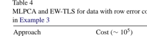
In calibration problems[32], the rows of the data matrix are formed by individual spectra. Hence, it is reasonable to discuss the case where correlations between the measurement errors exist only along the rows. So, the errors are uncorre-lated along the columns of the data matrix. In these cases the full covariance matrix W of the matrix of measurement errors will be block diagonal and can be stored as a sparse matrix. To calculate the inverse of W the diagonal blocks can be in-verted individually. For the discussion of this specific class of measurement structure a simulated data set from chemical measurements is used which was previously described in a paper by Wentzell and Lohnes[32].
Example 3. The simulated data set contained spectra from
10 samples of three-component mixtures. The concentration of each component in each of the 10 mixtures had a value
be-tween 0 and 1 from a uniform random number distribution. The spectral profiles of the three components were Gaus-sian with a standard deviation of 20 nm and maximum mo-lar absorptivities at 480, 500 and 520 nm, respectively. Pure spectral vectors were generated between 400 and 600 nm at 20 nm intervals. The noise-free data matrixD0was calcu-lated by multiplying the 10×3 matrix of concentrations by the 3×11 matrix of pure component spectra. To add a noise matrixDof correlated measurement errors to the noise-free matrixD0, first a 10×11 matrixDof uncorrelated measure-ment errors was generated. The matrix of the measuremeasure-ment standard deviations corresponding to this 10×11 matrix is determined by generating a 10×11 matrix of uniform dis-tributed random numbers between 0 and 0.01. This ensures that there is no pattern in the standard deviation matrix. Now, the 10×11 matrix of uncorrelated measurement errorsD is generated by taking a 10×11 random matrix with nor-mally distributed elements (with Matlab’srandn) and multi-plying this, element-wise, by the standard deviation matrix. To introduce correlations among the errors within the rows, the rows of matrixD were filtered using a 1×5 moving average digital filter (see[31, Eqs. (34)–(36)] for the def-inition) to construct the correlated error matrix D. This error matrixDw as added to the noise-free partD0in or-der to complete the noisy data matrixD=D0+Dof size 10×11.
EW-Fig. 2. The cost function value per iteration number is displayed for the MLPCA and the EW-TLS approaches applied to data with row error covariance only as described inExample 3.
[image:12.842.107.483.365.718.2]Table 4
MLPCA and EW-TLS for data with row error covariance only as described inExample 3
Approach Cost (∼105) Relative error mlpca 0.00058253884923 0.00472272972683 mlpca(gtls) 0.00058233611546 0.00468049099448 ewtlsAlgorithm 3 9.21164965017561 0.44610730154588 ewtls(opt)Algorithm 5 0.00058356157547 0.00478011794589
TLS algorithms are not yet optimized for handling corre-lated measurement errors in data sets where mN, as is the case here (see Note 6), we nevertheless applied it to this data set. After all, from the previous section it is clear that the EW-TLS approach can be very useful for chemometrical problems. We compare the cost which is de-fined by vec(D−Dˆ)W−1vec(D−Dˆ) and the relative er-ror D0−Dˆ F
D0 F . The results are presented inTable 4. The table
contains the results of applying the MLPCA approach with two different initial starting points. For the ‘mlpca’ approach the truncated SVD solution (see Note 2) is used. For the ‘mlpca(gtls)’ approach the GTLS approximation (Algorithm 1) is used as initial value instead of the truncated SVD solu-tion. We expect that the MLPCA algorithm with the GTLS approximation as initial value needs fewer iterations to con-verge.Fig. 2shows this is indeed the case.Table 4also con-tains the results of applying the EW-TLS approach with two different algorithms. These are the same as in the previous section. For ‘ewtls’Algorithm 3is used and for ‘ewtls(opt)’
Algorithm 5is applied to the data. For both algorithms we have used the GTLS approximation as initial starting point. From the table it is obvious that we obtain the same solution as the MLPCA algorithms with the ‘ewtls(opt)’ algorithm.
Fig. 2 contains the results of the computation time of the MLPCA and the EW-TLS approaches. The ‘mlpca(gtls)’ ap-proach performs the best for this specific case of measurement error and matrix size. As said before, the EW-TLS method needs to be optimized for this kind of data set.Fig. 2shows that it is better to use the GTLS approximation as initial value for the MLPCA algorithm.
5. Conclusions
In this paper we explored the tight equivalences between MLPCA and EW-TLS. We have shown that both methods can be used in any multivariate (ML) regression/calibration problemXB≈Yby reducing the problem to the same math-ematical kernel problem, i.e.finding the closest (in a cer-tain sense) weighted low rank matrix approximation where the weight is derived from the distribution of the errors in the data. Different solution approaches, as used in MLPCA and EW-TLS, have been discussed. From these discussions we can conclude that it is better to use the GTLS approx-imation as initial value for the MLPCA algorithm instead of the truncated SVD. Moreover, we have applied the EW-TLS algorithm to chemometrical data. The simulations show
that the EW-TLS method certainly has potential for the problems in chemometrics. EW-TLS outperforms MLPCA for data sets with unequal row error variances. Neverthe-less, a strong point of the MLPCA approach is its good convergence. But, the current algorithm is computation-ally not very efficient. Future work will focus on improv-ing the computational efficiency of MLPCA by combinimprov-ing its good convergence with the efficiency of the EW-TLS algorithm.
Acknowledgements
Prof. Dr. Sabine Van Huffel is a full professor, Mieke Schuermans and Ivan Markovsky are research assistants at the Katholieke Universiteit Leuven, Belgium. Prof. Dr. Peter D. Wentzell is a professor at the Dalhousie University, Canada, sponsored by the NSERC Canada and the Dow Chemical Company. Our research is supported by: Research Council KUL: GOA-Mefisto 666, IDO /99/003 and /02/009 (Predic-tive computer models for medical classification problemsus-ing patient data and expert knowledge), several PhD/postdoc & fellow grants; Flemish Government: FWO: PhD/postdoc grants, projects, G.0078.01 (structured matrices), G.0407.02 (support vector machines), G.0269.02 (magnetic resonance spectroscopic imaging), G.0270.02 (nonlinear Lp approxi-mation), research communities (ICCoS, ANMMM); IWT: PhD Grants; Belgian Federal Government: IUAP V-22 (2002-2006): Dynamical Systems and Control: Computation, Iden-tification & Modelling; EU: PDT-COIL, BIOPATTERN, ETUMOUR;
References
[1] R.J. Adcock, A problem in least squares, The Analyst 4 (1877) 183– 184.
[2] G.H. Golub, C.F. Van Loan, An analysis of the total least squares prob-lem, SIAM J. Numer. Anal. 17 (1980) 883–893.
[3] S. Van Huffel, J. Vandewalle, The Total Least Squares Problem: Com-putational Aspects and Analysis, SIAM, Philadelphia, 1991. [4] S. Van Huffel (Ed.), Recent Advances in Total Least Squares
Tech-niques and Errors-in-Variables Modeling, SIAM Proceedings Series, SIAM, Philadelphia, 1997.
[5] S. Van Huffel, P. Lemmerling (Eds.), Total Least Squares and Errors-in-Variables Modeling: Analysis, Algorithms and Applications, Kluwer Academic Publishers, Dordrecht, 2002.
[6] G.H. Golub, Some modified matrix eigenvalue problems, Siam Rev. 15 (1973) 318–344.
[7] G.H. Golub, C.F. Van Loan, Matrix Computations, 3rd ed., The Johns Hopkins University Press, Baltimore, 1996.
[8] C.-L. Cheng, J.W. Van Ness, Statistical Regression With Measurement Error, Arnold, London, 1999.
[9] W.A. Fuller, Error Measurement Models, Wiley, New York, 1987. [10] L.J. Gleser, Estimation in a multivariate “errors in variables” regression
model: large sample results, Ann. Statist. 9 (1981) 24–44.
[11] R.D. Degroat, E.M. Dowling, The data least squares problem and chan-nel equalization, IEEE Trans. Sign. Process. 41 (1993) 407–411. [12] S. Van Huffel, J. Vandewalle, Analysis and properties of the generalized
[13] R.D. Fierro, G.H. Golub, P.C. Hansen, D.P. O’Leary, Regularization by truncated total least squares, SIAM J. Sci. Comp. 18 (1997) 1223– 1241.
[14] D. Sima, S. Van Huffel, G.H. Golub, Regularized total least squares based on quadratic eigenvalue problem solvers, BIT (2004), in press. [15] K.S. Arun, A unitarily constrained total least-squares problem in
signal-processing, SIAM J. Matrix Anal. Appl. 13 (1992) 729–745. [16] T.J. Abatzoglou, J.M. Mendel, G.A. Harada, The constrained total least
squares technique and its applications to harmonic superresolution, IEEE Trans. Acoust. Speech Sign. Process. 39 (1991) 1070–1087. [17] A. Kukush, I. Markovsky, S. Van Huffel, Consistency of the structured
total least squares estimator in a multivariate model, J. Statist. Plann. Inference (2004), in press.
[18] N. Mastronardi, P. Lemmerling, S. Van Huffel, Fast regularized struc-tured total least squares algorithm for solving the basic deconvolution problem, Numer. Lin. Alg. Appl. (2002), in press.
[19] A. Premoli, M.L. Rastello, The parametric quadratic form method for solving problems with element-wise weighting, in: S. Van Huffel, P. Lemmerling (Eds.), Total Least Squares and Errors-in-Variables Mod-eling: Analysis, Algorithms and Applications, Kluwer, 2002, pp. 67– 76.
[20] I. Markovsky, M.L. Rastello, A. Premoli, A. Kukush, S. Van Huffel, The element-wise weighted total least squares problem, Comp. Stat. Data Anal., in press.ftp://ftp.esat.kuleuven.ac.be/pub/ SISTA/markovsky/abstracts/02–48.html.
[21] A. Kukush, S. Van Huffel, Consistency of elementwise-weighted to-tal least squares estimator in a multivariate errors-in-variables model AX=B, Metrika 59 (1) (2004) 75–97.
[22] S. Wold, A. Ruhe, H. Wold, W.J. Dunn, The collinearity problem in lin-ear regression. The partial least squares (PLS) approach to generalized inverses, SIAM J. Sci. Stat. Comput. 5 (3) (1984) 735–743. [23] A. Burnham, R. Viveros, J. MacGregor, Frameworks for latent variable
multivariate regression, J. Chemomet. 10 (1996) 31–46.
[24] S. de Jong, PLS fits closer than PCR, J. Chemomet. 7 (1993) 551– 557.
[25] S. de Jong, Regression coefficients in multilinear PLS, J. Chemomet. 12 (1) (1998) 77–81.
[26] A. Phatak, Evalauation of some multivariate methods and their appli-cations in chemical engineering, Ph.D. Thesis, University of Waterloo, 1993.
[27] A. Phatak, S. de Jong, The geometry of partial least squares, J. Chemomet. 11 (4) (1997) 311–338.
[28] P.D. Wentzell, D.T. Andrews, B.R. Kowalski, Maximum like-lihood multivariate calibration, Anal. Chem. 69 (1997) 2299– 2311.
[29] H. Martens, T. Naes, Multivariate Calibration, Wiley, New York, 1989.
[30] E.V. Thomas, Errors-in-variables estimation in multivariate calibration, Technometrics 33 (1991) 405–413.
[31] P.D. Wentzell, D.T. Andrews, D.C. Hamilton, K. Faber, B.R. Kowalski, Maximum likelihood principal component analysis, J. Chemomet. 11 (1997) 339–366.
[32] P.D. Wentzell, M.T. Lohnes, Maximum likelihood principal com-ponent analysis with correlated measurement errors: theoretical and practical considerations, Chemomet. Intell. Lab. Syst. 45 (1999) 65– 85.
[33] J.T. Webster, R.F. Gunst, R.L. Mason, Latent root regression analysis, Technometrics 16 (1974) 513–522.
[34] R.F. Gunst, J.T. Webster, R.L. Mason, A comparison of least squares and latent root regression estimators, Technometrics 18 (1976) 75– 83.
[35] W. Li, J. Qin, Consistent dynamic PCA based on errors-in-variables subspace identification, J. Process Contr. 11 (2001) 661– 678.
[36] J.H. Manton, R. Mahony, Y. Hua, The geometry of weighted low rank approximations, IEEE Trans. Sign. Process. 51 (2) (2003) 500– 514.