ClassifyingRNA pseudoknotted structures
Anne Condon
a;∗, Beth Davy
a, Baharak Rastegari
a, Shelly Zhao
a,
Finbarr Tarrant
baDepartment of Computer Science, University of British Columbia, Vancouver, BC, Canada V6T 1Z4 bThe Kane Building, Department of Computer Science, University College Cork, College Road, Ireland
Abstract
Computational prediction of the minimum free energy (mfe) secondary structure of an RNA molecule from its base sequence is valuable in understandingthe structure and function of the molecule. Since the general problem of predicting pseudoknotted secondary structures is NP-hard, several algorithms have been proposed that /nd the mfe secondary structure from a restricted class of secondary structures. In this work, we order the algorithms by generality of the structure classes that they handle. We provide simple characterizations of the classes of structures handled by four algorithms, as well as linear time methods to test whether a given secondary structure is in three of these classes. We report on the percentage of biological structures from the PseudoBase and Gutell databases that are handled by these three algorithms.
c
2003 Published by Elsevier B.V.
Keywords:RNA secondary structure; Pseudoknots; Classi/cation of structures
1. Introduction
RNA molecules—sequences of nucleic acid bases—play diverse roles in the cell: as carriers of information, catalysts in cellular processes, and mediators in determining the expression level of genes [5]. The structure of RNA molecules is often key to their
function, and so tools for computational prediction of RNA secondary structure—the
set of base pairings present in its folded state—are widely used.
While comparative approaches are most reliable for secondary structure
predic-tion [4], these approaches require that several homologous (i.e. evolutionarily and
functionally related) sequences are available. When just a single molecule is avail-able, computational prediction of its secondary structure from its base sequence (at
∗Correspondingauthor.
E-mail address:[email protected](A. Condon).
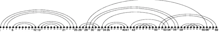
Fig. 1. Arc representation of an RNA secondary structure. In the left substructure (up to index 25), arcs are hierarchically nested, thus this is apseudoknot-freesubstructure. Arcs cross in the substructure on the right, thus it ispseudoknotted.
/xed temperature, ionic concentration, and pressure) is based on the premise that out of the exponentially many possibilities, an RNA molecule is most likely to fold into the minimum free energy (mfe) structure. The free energy of a given structure for a se-quence is estimated by summingthermodynamic and entropic free energy terms asso-ciated with the component loops of the secondary structure. Some of these terms have been obtained experimentally, and others are estimated based on existingdatabases of naturally occurringstructures.
Unfortunately, /ndingthe mfe secondary structure for a given RNA sequence is NP-hard [9]. Several polynomial time algorithms have been proposed for predicting the mfe secondary structure from restricted classes of secondary structures. The most well
known such class is that of pseudoknot-free secondary structures (see Fig. 1). Many
biological RNA structures are pseudoknot free and extensive experimental work has been done to determine parameters for the underlyingthermodynamic model. Pseudo-knot-free secondary structures can be described as generalized strings of balanced parentheses. Dynamic programming algorithms for /nding the mfe pseudoknot-free
sec-ondary structure from the base sequence run in E(n3) time, and are the basis for the
well-known mfold and Vienna secondary structure prediction packages [7,10].
More-over, there are linear time methods to test that a secondary structure (represented as an ordered list of base pairs or stems) is pseudoknot free, and to calculate the free energy of a given secondary structure for a given sequence. The latter algo-rithm is quite useful in practice, and software to do it available as part of the mfold package.
Pseudoknots occur in many natural structures [10,11]. Recently, algorithms have been designed to predict the mfe secondary structure for limited classes of pseudoknotted structures [1,6,8,11,13]. The running times of these algorithms range from E(n4) to
E(n6), and each handles a diGerent class of structures. However, the trade-oG between
the running time of the algorithms and the generality of the classes of structures they
handle has been poorly understood. Rivas and Eddy [11] state that “we still lack a
structures handled by these algorithms includes most known pseudoknotted biological structures.
To address these problems, in Section 3 we provide simple characterizations of the classes of structures handled by four algorithms: the Rivas and Eddy (R&E) class (which is the most general class known to us), the class of Akutsu and Uemura et al. (A&U) [13,1], the Dirks and Pierce (D&P) [6] class, and a simple class, modeled after that of LyngsHand Pedersen (L&P). Usingour characterizations, we provide linear time algorithms to test if an input structure is in the R&E, D&P, and L&P classes, and present results for several RNA secondary structure families. As an example of our results, in tests of 486 secondary structures with isolated base pairs removed, we found that all but three Group II Intron structures are in the R&E class.
We provide background on RNA secondary structure in Section5, and describe our
results in more detail in subsequent sections.
2. Secondary structure background
An RNA molecule is a chain of four types of bases, denoted by A, C, G, and U
(for Adenine, Cytosine, Guanine, and Uracil). The chain has distinct 5 and 3 ends.
We index the bases consecutively from the 5 end, startingat 1. A folded molecule
is held together by hydrogen bonds between pairs of bases, with each base typically
participatingin at most one pair. A set R of such base pairs is called a secondary
structure of the molecule. If bases indexed i and j are paired where i¡j then we write i·j∈R. Throughout, we use n to denote the length of a molecule.
Fig. 1 gives an arc representation of a secondary structure. The chain of indexed
bases is represented as an indexed line of dots, and arcs connect paired bases. Later, we will use a linked list representation of secondary structures, where list elements are the
base indices, ordered startingfrom the 5 end, with additional pointers corresponding
to arcs of the structure’s arc representation.
We will also use an alternative pattern representation of secondary structures. In
a pattern, information about the base indices is lost but the pattern of nestingor overlaps amongbase pairs is preserved. (We note that the de/nition of pattern could be extended so that unpaired bases are represented usinga special symbol.) To de/ne
patterns precisely, we introduce some notation. We use to denote the empty string.
LetNn denote the natural numbers between 1 andn (inclusive). For any string sover
alphabet , s↓ denotes the string s with all occurrences of removed. Also, |s|
denotes the number of symbols in s.
Patterns: A stringp (of even length) over some alphabetis asecondary structure pattern, or simply a pattern, if every symbol of occurs either exactly twice, or not at all, in p. We say that secondary structure Rfor a strand of lengthn corresponds to
pattern p if there exists a mapping m:Nn →∪ {} with the followingproperties:
(i) if i·j∈R then m(i)∈ and m(i) =m(j), (ii) if i·j and j·i =∈R for all j∈Nn,
thenm(i) =, and (iii) p=m(1)m(2): : : m(n). For example, the substructure of Fig.1
from indices 5 to 21 corresponds to pattern ABBACDEEDC, and the substructure
between commonly used representations of secondary structures, such as list of base pairs, and pattern representations, in time linear in n.
Let R⊆N2
n correspond to pattern p over alphabet and let mapping m
wit-ness this correspondence. Let m−1
i : → Nn be de/ned by m−1i () =
min{i∈Nn|m(i) =} ∪ {n+1}and letmj−1() = max{j∈Nn|m(j) =} ∪ {0}. Note
that m−1
i ()∈Nn if and only if m−1j ()∈Nn, in which casem−1i ()¡m−1j (). Also,
(m−1
i (); m−1j ()) = (n+ 1;0) if and only if does not occur in patternp. If (m−1i ();
m−1
j ())= (n+ 1;0) thenm−1i ()·m−1j ()∈R and we say that base pairm−1i ()·m−1j
() corresponds to .
Fig. 1 illustrates a pseudoknot free substructure (up to index 25) and a
pseudo-knotted substructure. Formally, a secondary structure R is pseudoknot free if for all
pairs i·j and i·j in R, it is not the case that i¡i¡j¡j. Applyingthis de/nition
directly to determine whether a secondary structure is pseudoknot free would require
E(n2) time. However, linear time tests for pseudoknot freeness are well known. For
completeness, and because our characterizations of pseudoknotted secondary structure classes presented later are similar, we outline such a test here. We use the notion of pseudoknot free patterns.
Pseudoknot free patterns: We say that symbolisself-adjacentin stringpifis a
substringof p. We write p−→
PKFp
if p=p↓, for some self-adjacent
symbol of p, and p−−→∗
PKF p
if p=p or ∃ patterns p
1; : : : ; pk for some k such
that p−→
PKFp1−→PKF· · ·pk−→PKFp
. We say that p is apseudoknot free pattern if and only
if p−−→∗ PKF .
It is straightforward to show that secondary structure R is pseudoknot free if and
only if the pattern correspondingto R is pseudoknot free. Roughly, a linear time test
that a pattern is pseudoknot free simply scans the pattern from left to right, removing self-adjacent pairs when possible. The pattern is empty after the last symbol is scanned, if and only if it is pseudoknot free.
3. Structure classes
Dynamic programming algorithms for prediction of mfe pseudoknotted secondary structures were proposed (in chronological order) by Uemura et al. [13], Akutsu [1], Rivas and Eddy (R&E) [11], LyngsH and Pedersen (L&P) [8], and Dirks and Pierce (D&P) [6]. (We note that the D&P algorithm is more general than the others, in that it can calculate the partition function as well as the mfe secondary structure.) Each algorithm /nds the mfe structure from a limited class of secondary structures. Akutsu derived his class by simplifyingthat of Uemura et al. We call the class, as described by Akutsu, the A&U class. We refer to the other classes by the initials of the au-thors of the algorithm. We note that our version of the L&P class is simpler than
that de/ned in their paper—see Section 3.4. We use PKF to denote the class of
follows:
PKF⊂L&P⊂D&P⊂A&U⊂R&E:
The fact that the A&U class is properly contained in the R&E class was already noted by LyngsH and Pedersen [9], by comparingthe structure of the recurrences of both algorithms. Instead, to derive our containments, in the next subsections we develop formal characterizations of each of the D&P and R&E classes. Precise descriptions of
the A&U and L&P classes are already in the work of Akutsu [1] and LyngsH and
Pedersen (L&P) [8], respectively, but we also characterize these classes in a manner similar to our characterizations of the D&P and R&E classes, so that the containments above can be derived.
3.1. R&E structures
The R&E structure class is de/ned implicitly by the recurrences of the algorithm of Rivas and Eddy [11]. We /rst abstract the form of the recurrences to de/ne the class of secondary structures that their class can handle; this is done formally in the de/nition of R&E-algorithm patterns below. Following this, we give our characterization of the structure class, and argue that our characterization is equivalent to the class of R&E-algorithm patterns.
We need to account for “gapped regions” that play an important role in the R&E
recurrences, and so we /rst introduce generalized patterns. A generalized patternover
is a string p over ∪ {G}, where G =∈, such that there is at most one G in
p and p↓G is a pattern. A generalized pattern p over alphabet is a generalized
R&E-algorithm pattern if at least one of the followingconditions hold. 1. p= or p=g, for some ∈ and g∈ {G; }.
2. p=Gp or p=pG wherep is a generalized R&E-algorithm pattern. 3. p=p1p2gp3p4 where|p|¿4, g∈[G; ], p1p2p3p4∈∗, and either
(a) p1Gp3 andp2Gp4 are generalized R&E-algorithm patterns,|p1Gp3|¡|p|, and |p2Gp4|¡|p|, or,
(b) p1Gp4 andp2gp3 are generalized R&E-algorithm patterns, |p1Gp4|¡|p|, and |p2gp3|¡|p|.
4. p=p1Gp2p3p4 or p=p1p2p3Gp4 where|p|¿4, p1Gp3 and p2Gp4 are gener-alized R&E-algorithm patterns, |p1Gp3|¡|p|, and |p2Gp4|¡|p|.
A generalized R&E-algorithm pattern p is a R&E-algorithm pattern if p does not contain G. We say that secondary structure R is an R&E secondary structure it cor-responds to a R&E-algorithm pattern.
We next de/ne the class of R&E patterns, which is a simple generalization of the pseudoknot free patterns. In Theorem 1 we will show that the set of R&E-algorithm patterns is equal to the set of R&E patterns. Letp be a stringover alphabet. Symbol
is directly adjacent to symbol in p if and only if either is a substringof p
or there are two disjoint substrings x; y of p, both of length 2, such that and are
both in x and and are both in y. (The direct adjacency relation is not necessarily
symmetric.) If is directly adjacent to some symbol in pattern p, we say is directly
Letpbe a pattern. We say thatp−−→ R&Ep
ifp=p↓for some that is either self-adjacent or directly self-adjacent in p. Also, p−−→∗
R&Ep
if p=p or ∃ patterns p 1; : : : ; pk
for some k such thatp−−→
R&Ep1−−→R&E· · ·pk−−→R&Ep
. Pattern p is R&E if p−−→∗ R&E. A generalized pattern p over ∪ {G} is a generalized R&E pattern if either p is R&E, p−−→∗
R&EG or p ∗ −−→
R&EG for some ∈.
Theorem 1. The R&E secondary structures are exactly the structures corresponding to R&E patterns.
Proof. We show one direction, that ifp is a generalized R&E-algorithm pattern, then p is a generalized R&E pattern. The proof is by induction on |p|. The base case is straightforward. For the inductive step, let |p|¿3, and suppose that all generalized R&E-algorithm patterns of length ¡|p| are R&E.
In the most interestingcase, p=p1p2gp3p4 where case 3(b) of the de/nition of R&E-algorithm patterns holds forp1; p2; p3andp4. Since|p1Gp4|¡|p|and|p2gp3|¡ |p|, it follows from the induction hypothesis that p1Gp4 and p2gp3 are generalized R&E patterns. The result therefore follows from the followingclaim.
Claim. If p1Gp4 and p2gp3 are generalized R&E patterns, where g∈[G; ] then p1p2gp3p4 is a generalized R&E pattern.
Claim can be also be proved in a straightforward way, by induction on |p1p2p3p4|. One base case is when for some and , =p1=p4 and =p2=p3, so that
p=g−−→
R&Eg, which is a generalized R&E pattern by the base case of the de/-nition of R&E patterns.
For the inductive step, let |p1p2p3p4|¿4 and suppose that the Claim holds for all p
1; p2; p3; p4 with |p1p2p3p4|¡|p1p2p3p4|. We consider the case where |p1p4|¿2; the case where|p2p3|¿2 is similar. Suppose thatp1Gp4−−→
R&Ep
1Gp4, wherep1Gp4 is a generalized R&E pattern. Then, by the induction hypothesis, since|p
1Gp4|¡|p1Gp4|, p
1p2gp3p4 is a generalized R&E pattern. Also, p1p2gp3p4−−→ R&Ep
1p2gp3p4, since if is self-adjacent or directly adjacent in p1gp4 then must also be self-adjacent or directly adjacent in p1p2gp3p4. Therefore,
p1p2gp3p4−−→R&Ep1p2gp3p4−−→R&E∗ ;
from which the Claim follows. 3.2. A&U et al. structures
We /rst de/ne the A&U structure class, followingthe de/nition of Akutsu [1].
A secondary structure R is called a simple pseudoknot if there exist j
0; j0∈Nn with
j
0¡j0 for which the followingconditions are satis/ed.
1. Each i·j∈R satis/es either i¡j
06j¡j0 or j06i¡j06j. 2. If i·j andi·j are in R with either i¡i¡j
R is an A&U secondary structure if either R is a simple pseudoknot or a pseudoknot free secondary structure, or for some i0; k0; 16i0¡k06n; R=R∪R where R⊆ (Nn−[i0; k0])2, R⊆[i0; k0]2, R is an A&U structure and R is a nonempty simple pseudoknot or pseudoknot free structure.
Our characterization of A&U structures is less elegant than that obtained for the R&E class in the previous section, but is nevertheless useful in order to compare the classes.
Letpbe a string. We say thatisdirectly nested inp,with respect to, if disjoint substringsandappear inpin that order. Ifis directly nested inp, with respect to some , we say that is directly nested in p. We say that is A&U-adjacent in p, with respect to if is directly nested in p or if substring is followed (not necessarily contiguously) by substring inp.
Given , we say p−−−→ A&U; p
if p=p↓ for some that is A&U-adjacent in p with respect to . We say p−−−→∗
A&U; p
if for some k¿0, ∃ patterns p
1; : : : ; pk such that
p−−−→
A&U; p1−−−→A&U; · · ·pk−−−→A&U; p
, and moreover, is self-adjacent in p. We say thatp−−→
A&Up
ifp=p↓for some that is self-adjacent or directly nested inpor ifp−−−→∗
A&U; p
for some. We say thatp →∗ A&Up
ifp=p or∃patternsp1; : : : ; pk such that p−−→
A&Up1−−→A&U · · · spk−−→A&Up
. Pattern p is A&U if p →∗ A&U.
Theorem 2. The A&U secondary structures are exactly the structures corresponding to A&U patterns.
Proof. We include the direction that every A&U secondary structure corresponds to an A&U pattern. Let R be an A&U secondary structure. Firstly, if R is pseudoknot free, then its correspondingpattern is a pseudoknot free pattern, and therefore an A&U pattern, since the −−→
A&U relation generalizes the −→PKF relation.
Secondly, suppose that R is a simple pseudoknot, but is not pseudoknot free. Let p be the pattern correspondingto R. Let p be obtained from p by repeatedly removing any self-adjacent symbols and let R be the substructure of R obtained by removing the base pairs correspondingto these self-adjacent symbols. Let be the /rst symbol in p. Let i·j be the base pair of R correspondingto . Then, since R is not pseu-doknot free, by condition 1 of the de/nition of a simple pseupseu-doknot it must be that i6j
06j¡j0. Moreover, condition 1, together with the fact that p contains no self-adjacent base pairs, implies that for all other base pairsi·j, either (i)i¡i¡j¡j¡j
0 or (ii) j
06i¡j¡j06j.
Let be the symbol just to the left of the second occurrence of in p, and let i·j be the base pair of R correspondingto . Then, either i·j satis/es case (i) of the last paragraph, in which case is directly nested in p with respect to , or i·j satis/es case (ii) of the last paragraph, in which case is a substringof p. In either case, is A&U-adjacent to in p, and so p−−−→
A&U; p
then by the same reasoningas for , it must be that p−−−→ A&U; p
↓. Continuingin this way, we conclude that p−−−→∗
A&U; .
Therefore, p →∗
A&U by a series of steps in which /rst self-adjacent symbols are re-moved, then symbols that are A&U adjacent to the /rst symbol of p are removed, and /nally −−→
A&U. Therefore, p is an A&U pattern.
Finally, suppose thatR is an A&U secondary structure that is neither a simple pseu-doknot nor pseupseu-doknot free. Then, for some i0; k0; 16i0¡k06n; R=R∪R where R⊆(N
n−[i0; k0])2, R⊆[i0; k0]2, R is an A&U structure and R is a nonempty simple pseudoknot or pseudoknot free structure. Let p; p, andp be the patterns cor-respondingto R; R, and R, respectively. A proof by induction can be used to show that if p and p are A&U patterns, then so is p; in fact p →∗
A&Up ∗→
A&U. Therefore R corresponds to an A&U pattern.
3.3. D&P structures
As with the R&E structure class, the D&P structure class is also de/ned implicitly, in this case by the recurrences of the algorithm of Dirks and Pierce [6]. We abstract the form of the recurrences to de/ne the class of secondary structures that their class can handle; this is done formally in the de/nition of D&P-algorithm patterns below, which is in fact a restriction of the recurrences of Rivas and Eddy. (Our abstraction does not capture certain features of their algorithm, that are important in the context of their work, but not important in terms of de/ningthe class of structures handled.) Followingthis, we give our characterization of the D&P structure class.
A generalized pattern pover alphabet is a generalized D&P-algorithm patternif
at least one of the followingconditions hold. 1. p= or g, for some ∈ and g∈ {G; }.
2. p=Gp or pG wherep is a generalized D&P-algorithm pattern.
3. p=p1 for some ∈, where p1 is a generalized D&P-algorithm pattern. 4. p=p1p2p3p4 where |p|¿4, p∈∗, p1Gp3 and p2Gp4 are generalized
D&P-algorithm patterns, |p1Gp3|¡|p|, and |p2Gp4|¡|p|. 5. p=p1p2Gp3p4 where|p|¿4 and either
(a) p2Gp3p4 andp1 are generalized D&P-algorithm patterns,|p2Gp3p4|¡|p|and |p1|¡|p|, or,
(b) p1p2Gp3 andp4 are generalized D&P-algorithm patterns,|p1p2Gp3|¡|p|and |p4|¡|p|.
A generalized D&P-algorithm pattern p is a D&P-algorithm pattern if p does not contain G. We say that secondary structure R is an D&P secondary structure it corresponds to a D&P-algorithm pattern.
We next de/ne the class of D&P patterns. Letpbe a string. We say thatp−−→ D&Pp
if p=p↓ for some that is self-adjacent or directly nested in p, or ifp= (p↓)↓ for some symbols and such that the substring is in p. p−−→∗
D&Pp
or ∃ patterns p1; : : : ; pk such that p−−→D&Pp1−−→D&P· · ·pk−−→D&Pp. Pattern p is D&P if
p−−→∗ D&P.
Theorem 3. The D&P secondary structures are exactly the structures corresponding to D&P patterns.
The proof of Theorem 3 is similar in spirit to that of Theorem 1.
3.4. L&P structures
LyngsH and Pedersen [8] outline a dynamic programming algorithm for a restricted
class of structures. The class includes structures of the form s1s2s1s2 where both
s1s1 and s2s2 are pseudoknot free. We call such structures L&P structures.
Simi-lar to the characterizations above, we can also describe the L&P structure class as follows.
Letpbe a string. We say thatp−−→
D&Pp
ifp=p↓for somethat is self-adjacent
or directly nested in p, or if p= and p=. p→∗
L&Pp
if p=p or ∃ patterns
p1; : : : ; pk such that p−−→
L&P p1−−→L&P · · ·pk−−→L&P p
. Pattern p is L&P if p→∗
L&P.
Sec-ondary structureRisa L&P secondary structureif it corresponds to a L&P patternp. The followingtheorem follows easily from the above de/nitions.
Theorem 4. The L&P structure class is exactly the set of L&P secondary structures.
The algorithm outlined by LyngsH and Pedersen can also handle structures of the form s1s2s1s2s1 where both s1s1s1 and s2s2 are pseudoknot free. We call this class L&P+. Lyngso and Pedersen [9] note that PKF⊂L&P+⊂R&E. However, L&P+ is
incomparable with the D&P and A&U classes, since ABACBC is in L&P+ but not in
A&U, whileABCDCDABis in D&P but not in L&P+. In what follows, we work with
the simpler L&P class.
3.5. Containments between the classes
We can now prove the followingtheorem:
Theorem 5.
PKF ⊂L&P⊂D&P⊂A&U ⊂R&E:
Proof. Consider each of −→
Therefore,
p−−→∗ PKF p
⇒p→∗ L&Pp
⇒p−−→∗ D&Pp
⇒p →∗ A&Up
⇒p−−→∗ R&Ep
:
From our characterizations, it follows that the followingpatterns separate the classes (details omitted): (i) ABAB is in L&P - PKF, (ii) ABCBCA is D&P - L&P, (iii) ABCBDADC is A&U - D&P [6], and (iv) ABCABC is R&E - A&U [6]. Also, ABCADBECDE is not R&E [11].
4. Testing membershipin structure classes
We have developed linear-time tests for membership in the R&E, D&P, and the L&P classes. Here, we describe the algorithms, and report on the results of applying the algorithms on several biological structures.
4.1. A linear time algorithm to recognize R&E structures
Algorithm 1 tests if a pattern over some /xed alphabet is a R&E pattern. The
pattern is scanned from the left and the −−→
R&E operation is applied when possible. In
the algorithm, is a symbol variable over ∪ {} andpL andpR are stringvariables
over∗. Letsands be stringvariables over∗. Ifs=
12· · ·k with alli∈and
k¿1, then we de/ne the operations←s to set to
1 ands to2· · ·k. Similarly,
the operation s ← s sets to
k and s to 1· · ·k−1. If s= then the operations
s←s ands←s set=s=.
Algorithm 1. A test for R&E patterns algorithm R&E-Pattern-Test
input: pattern p=12· · ·sk∈k with k¿2
output: yes, if p is an R&E pattern and no otherwise pL←; ←1; pR ←2· · ·sk;
repeat
if some is directly adjacent to then arbitrarily choose any such ; pL←pL↓; pR←pR↓;
elseif is self-adjacent or directly adjacent then p
L←pL↓; pR←pR↓;
if p
L=then pL←pL; pR ←pR
else pR←pR; pL←pL;
else pL←pL; pR←pR;
until =;
If the pattern is stored as a doubly linked list of symbols, with additional links between the two instances of each symbol, then each iteration of the repeat loop can be implemented in O(1) time. Thus, the total time is O(k) on an input pat-tern of length k. In Theorem 6, we prove that algorithm R&E-Pattern-test recog-nizes exactly the R&E patterns. The followinglemma is key to the proof:
Lemma 1. Let p be a R&E pattern and let p−−→
R&Ep↓. Then p↓ is R&E.
Proof. Suppose thatp=p0−−→R&Ep1· · · −−→R&Epk−−→R&E. Let i be such that pi=pi−1↓. The proof is given in two cases.
First, suppose that is self-adjacent in p, or that is directly adjacent to in p, where ∈pi. Then we claim that
p↓=p0↓−−→
R&Ep1↓−−→R&E · · ·spi−1↓=pi−−→R&E · · ·spk↓−−→R&E; (1) from which the lemma follows. To see why (1) is true, /x any j; 16j¡i and let
pj=pj−1↓. We need to show that pj−1↓−−→R&Epj↓. If is self-adjacent or
di-rectly adjacent to some = in pj−1, then it is also the case that is self-adjacent
or directly adjacent to some = in pj−1↓, and so pj−1↓−−→R&Epj↓.
Other-wise, it must be that is directly adjacent to in pj−1. Then if is self-adjacent
in p, is a substringof pj−1, in which case is self-adjacent in pj−1↓. If
is a substringof p for some , then is a substringof pj−1↓, in which
case is directly adjacent in pj−1↓. Finally, if p contains two disjoint substrings
x; y, both of length 2, such that for some , and are both in x and and
are both in y, and ∈pi then pj−1↓ must contain two substrings x; y, both of
length 2, such that and are both in x and and are both in y, in which
case again is directly adjacent to in pj−1↓. In all cases, we can conclude that
pj−1↓−−→R&Epj↓.
Second, suppose that p contains two disjoint substrings x; y, both of length 2, such
that for some , and are both in x, and are both in y, and is not in pi.
Let h be such that ph=ph−1↓ , where h¡i. For h6l6i−1, let ph be obtained by
replacing with . Note that ph−1↓=ph and pi−1−−→R&Epi−1↓ =pi. In this case
we claim that
p↓=p0↓−−→
R&E: : : ph−1 ↓
=p
h−−→R&Eph+1−−→R&E· · ·pi−1−−→R&Epi−−→R&Epi+1−−→R&E· · ·pk↓−−→R&E:
To see why, for j¡h, the argument that pj−1↓−−→
R&Epj↓ is as in the /rst case
above. It remains to show that for h¡j6i−1, p
pj=pj−1↓, (so that also pj=pj−1↓). If is directly adjacent to in pj−1, then is directly adjacent to inp
j−1, in which case pj−1−−→R&Epj.
Theorem 6. Algorithm R&E-pattern-test outputs yes on input p if and only if p is R&E.
Proof. Letp(Li),(i), andp(i)
R be the values of variablespL; , andpR at the end of the
ith iteration of the repeat loop. Letlbe the total number of iterations of the repeat loop (since at every iteration, either |pR| or |pL| decreases, the algorithm must halt). It is
straightforward to show that for eachi, 16i6l, eitherpL(i−1)(i−1)p(i−1)
R =p(Li)(i)p(Ri) or
p(Li−1)(i−1)p(i−1)
R −−→R&Ep(Li)(i)p(Ri).
Also, if the algorithm returns yes, then p(Ll)(l)p(l)
R =. Therefore, if the algorithm
returns yes, p is R&E.
If the algorithm returns no, then|p(Ll)|¿0 and also(l)p(l)
R =. Therefore,p−−→R&E∗ p(Ll).
From Lemma 1 it follows that if pL(l) is not R&E, then p is not R&E. To show that
p(l)L is not R&E we show that the followinginvariant is true for each i; 06i6l. Invariant: No symbol is self-adjacent inp(i)L , and if any symbolis directly adjacent in p(i)L then(i) is a substringof p(i)
L .
Since p(0)L =, the invariant is true for i= 0. Suppose the invariant is true for
i−1. We show that it is true for i. It is straightforward to show that if p(i)L is a pre/x of p(iL−1), then the invariant holds for i. Otherwise, it must be the case that for some , either (i−1) or (i−1) (or both) is in p(i−1)
L , pL(i)=p(iL−1)↓, and
(i)=(i−1).
Let# and$ be the symbols (if any) just before and just after(i−1) inp(i)
L . Then#
and$ are the only symbols which could possibly be self-adjacent or directly adjacent
in p(i)L but not in p(iL−1). Since the only change to # and$ is that now (i−1) is their
neighbour, and since neither # nor $ can equal (i−1), they cannot be self-adjacent.
However, if #=$ then # is directly adjacent to (i−1), because #i−1# is a substring
of p(i)L . Therefore, since (i)=(i−1), the invariant holds for i. From the invariant, we
conclude that no symbol inp(l)L is self-adjacent or directly adjacent. Therefore, p(l)L is not R&E.
4.2. Linear time algorithms to recognize D&P and L&P structures
Algorithms 2 and 3 test for membership in the D&P and L&P structure classes,
respectively. They are very similar to Algorithm 1, and their correctness proofs are
Algorithm 2. A test for D&P patterns algorithm D&P-Pattern-Test
input: pattern p=12: : : k∈k with k¿2
output: yes, if p is a D&P pattern and no otherwise
pL←; ←1; pR←2: : : k;
repeat
if some is directly nested with respect to then pL←pL↓; pR←pR↓;
elseif is self-adjacent then p
L←pL↓; pR←pR↓;
if p
L= then pL←pL; pR←pR
else pR←pR; pL←pL;
else if is a suRx of pL for some then
p
L←(pL↓)↓;
if p
L= then pL←pL; pR←pR
else pR←pR; pL←pL;
else pL←pL; pR←pR;
until =;
if pL= then return yes else return no.
Algorithm 3. A test for L&P patterns algorithm L&P-Pattern-Test
input: pattern p=12: : : k∈k with k¿2
output: yes, if p is an L&P pattern and no otherwise
pL←; ←1; pR←2: : : k;
repeat
if some is directly nested with respect to then pL←pL↓; pR←pR↓;
elseif is self-adjacent then p
L←pL↓; pR←pR↓;
if p
L= then pL←pL; pR←pR
else pR←pR; pL←pL;
else pL←pL; pR←pR;
until =;
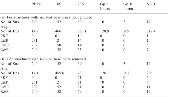
Table 1
Structure classi/cation
PBase 16S 23S Gp I Gp II NDB
Intron Intron (a) For structures with isolated base pairs not removed
No. of Strs 240 152 69 10 3 12
Avg.
No. of Bps 14.2 466 763.1 128.9 209 312.4
PKF 0 0 14 0 0 1
L&P 231 12 14 10 0 1
D&P 232 150 14 10 0 5
R&E 240 152 25 10 0 7
(b) For structures with isolated base pairs removed
No. of Strs 240 152 69 10 3 12
Avg.
No. of Bps 14.1 455.6 733 126.1 207 268
PKF 0 0 21 0 0 6
L&P 231 12 21 10 0 6
D&P 232 152 21 10 0 11
R&E 240 152 69 10 0 12
In each part, columns 2–7 present data for each RNA data set. For each data set (column), the entry in /rst row lists the number of structures in the data set. The second row lists the average number of base pairs in the structures once isolated base pairs are removed. The remainingrows list the number of structures of the data set that are in the PKF, L&P, D&P, and R&E classes, respectively.
4.3. Classi9cation of biological structures
We applied our algorithms to classify secondary structures from PseudoBase (PBase)
[2], the Nucleic Acids Database (NDB) [3], 16S and 23S ribosomal RNA and Groups I
and II Introns from the Gutell Database [4]. (We also considered 5S RNA secondary
structures, and all were pseudoknot free.) We considered only secondary structures with no occurrences of triple base stacking. Structures in these data sets may con-tain isolated base pairs, namely base pairs i·j such that neither (i+ 1)·(j−1) nor (i−1)·(j+ 1) is in the structure. Since isolated base pairs are sometimes consid-ered to be tertiary rather than secondary structure, we classi/ed the structures be-fore and after removal of the isolated base pairs. Our results are presented in Table 1.
5. Conclusions
Our characterizations of structure classes handled by RNA secondary structure pre-diction algorithms, and our tests for membership in these classes, provide the /rst means for evaluating the generality of current algorithms. The results show that current algorithms do in fact handle a wide range of known biological structures, though not all such structures.
There is a trade-oG between algorithm complexity and the generality of the class of structures that can be handled by the algorithm. An interesting question is whether faster algorithms can be found for any of the classes L&P, D&P, A&U, or R&E, or whether algorithms with comparable running times but that handle a more general (and biologically interesting) class of structures can be obtained.
In future work, we will develop a linear time algorithm for characterizing the A&U structure class.
Acknowledgements
We thank Mirela Andronescu, Matthew Cook, Robert Dirks, Holger Hoos, Niles Pierce, Joseph SchaeGer, Dan Tulpan, and Erik Winfree for valuable feedback on earlier versions of this work.
References
[1] T. Akutsu, Dynamic programming algorithms for RNA secondary structure prediction with pseudoknots, Discrete Appl. Math. 104 (2000) 45–62.
[2] F.H.D. Batenburg, A.P. van, Gu. ltyaev, C.W.A. Pleij, J. Ng, J. Oliehoek, Pseudobase: a database with RNA pseudoknots, Nucl. Acids Res. 28 (1) (2000) 201–204.
[3] H.M. Berman, et al., The mucleic acid database: a comprehensive relational database of three-dimensional structures of nucleic acids, Biophys. J. 63 (1992) 751–759.
[4] J.J. Cannone, et al., The comparative RNA web (CRW) site: an online database of comparative sequence and structure information for ribosomal, intron, and other RNAs, BioMed Central Bioinformatics 3 (2002) 2 (correction: BioMed Central Bioinformatics 3 (2002) 15).
[5] C. Dennis, The brave new world of RNA, Nature 418 (11) (2002) 122–124.
[6] R.M. Dirks, N.A. Pierce, A partition function algorithm for nucleic acid secondary structure including pseudoknots, J. Comput. Chem. 24 (13) (2003) 1664–1677.
[7] I.L. Hofacker, W. Fontana, P.F. Stadler, S.L. BonhoeGer, M. Tacker, P. Schuster, Fast foldingand comparison of RNA secondary structures, Monatsh. Chem. 125 (1994) 167–188.
[8] R.B. LyngsH, C.N. Pedersen, Pseudoknots in RNA secondary structures, Proc. 4th Ann. Internat. Conf. on Computational Molecular Biology (RECOMB), 2000, pp. 201–209.
[9] R.B. LyngsH, C.N. Pedersen, RNA pseudoknot prediction in energy-based models, J. Comput. Biol. 7 (3) (2000) 409–427.
[10] D.H. Mathews, J. Sabina, M. Zuker, D.H. Turner, Expanded sequence dependence of thermodynamic parameters improves prediction of RNA secondary structure, J. Mol. Biol. 288 (1999) 911–940. [11] E. Rivas, E.S.R. Eddy, A dynamic programming algorithm for RNA structure prediction including
pseudoknots, J. Mol. Biol. 285 (1999) 2053–2068.
[13] Y. Uemura, A. Hasegawa, S. Kobayashi, T. Yokomori, Tree adjoining grammars for RNA structure prediction, Theoret. Comput. Sci. 210 (1999) 277–303.