This is a repository copy of
Integrated optimization of mixed-model assembly sequence
planning and line balancing using Multi-objective Discrete Particle Swarm Optimization
.
White Rose Research Online URL for this paper:
http://eprints.whiterose.ac.uk/147016/
Version: Accepted Version
Article:
Ab Rashid, M.F.F., Tiwari, A. and Hutabarat, W. orcid.org/0000-0001-7393-7695 (2019)
Integrated optimization of mixed-model assembly sequence planning and line balancing
using Multi-objective Discrete Particle Swarm Optimization. AI EDAM. ISSN 0890-0604
https://doi.org/10.1017/S0890060419000131
This article has been published in a revised form in AI EDAM
[https://doi.org/10.1017/S0890060419000131]. This version is free to view and download
for private research and study only. Not for re-distribution, re-sale or use in derivative
works. © Cambridge University Press.
[email protected] https://eprints.whiterose.ac.uk/ Reuse
Items deposited in White Rose Research Online are protected by copyright, with all rights reserved unless indicated otherwise. They may be downloaded and/or printed for private study, or other acts as permitted by national copyright laws. The publisher or other rights holders may allow further reproduction and re-use of the full text version. This is indicated by the licence information on the White Rose Research Online record for the item.
Takedown
If you consider content in White Rose Research Online to be in breach of UK law, please notify us by
1
Integrated Optimisation of Mixed-Model Assembly Sequence Planning and Line
Balancing using Multi-Objective Discrete Particle Swarm Optimisation
Mohd Fadzil Faisae Ab Rashid
Corresponding Author
Faculty of Mechanical Engineering, Universiti Malaysia Pahang, 26600 Pekan, Malaysia
Email: [email protected]
Telephone: +609-4246321
Ashutosh Tiwari
Manufacturing and Materials Department, Cranfield University, Bedford, MK43 0AL, United
Kingdom.
Windo Hutabarat
Manufacturing and Materials Department, Cranfield University, Bedford, MK43 0AL, United
Kingdom.
Short title: Integrated Optimisation of Mixed-Model ASP and ALB using MODPSO
Number of pages: 31
Number of tables: 10
2
Abstract
Recently, interest in integrated Assembly Sequence Planning (ASP) and Assembly Line Balancing
(ALB) began to pick up because of its numerous benefits, such as the larger search space that leads to
better solution quality, reduced error rate in planning and expedited product time-to-market. However,
existing research is limited to simple assembly problem that only runs one homogenous product. This
paper therefore model and optimise the integrated mixed-model ASP and ALB using Multi-objective
Discrete Particle Swarm Optimisation (MODPSO) concurrently. This is a new variant of the integrated
assembly problem. The integrated mixed-model ASP and ALB is modelled using task based joint
precedence graph. In order to test the performance of MODPSO to optimise integrated mixed-model
ASP and ALB, an experiment using a set of 51 test problems with different difficulty levels was
conducted. Besides that, MODPSO coefficient tuning was also conducted to identify the best setting so
as to optimise the problem. The results from this experiment indicated that the MODPSO algorithm
presents significant improvement in term of solution quality towards Pareto optimal and demonstrates
ability to explore the extreme solutions in the mixed-model assembly optimisation search space. The
originality of this research is on the new variant of integrated ASP and ALB problem. This paper is the
first published research to model and optimise the integrated ASP and ALB research for mixed-model
assembly problem.
Keywords
Manufacturing systems, Assembly sequence planning, Line balancing, concurrent optimization, Particle
3
1. Introduction
Assembly Sequence Planning (ASP) and Assembly Line Balancing (ALB) are classified as important
activities in assembly optimisation although it occurs in different stages (Marian, 2003). Recently, there
are efforts to integrate and optimise both activities concurrently because of benefits of reduced planning
error and reduced costing in manufacturing (Tseng and Tang, 2006). The use of integrated scheme in
engineering provide huge benefits (Penciuc et al., 2016). A recent study that compared the sequential
and integrated optimisation approaches for ASP and ALB concluded the integrated approach is
preferable for better solution quality because of larger search space (Ab. Rashid, Tiwari and Hutabarat,
2017). Additionally, the integrated optimisation can also speed up time-to-market for a product (Lu and
Yang, 2016).
Assembly line problems are categorised into simple and generalised assembly line balancing problem
(Becker and Scholl, 2006). The simple assembly line balancing problem (SALBP) only considers the
production of one homogeneous product on serial line layout, while the generalised assembly line
balancing problem (GALBP) includes all of the problems that are not SALBP, such as mixed-model,
parallel, U-shaped and two-sided lines with stochastic dependent processing times (Tasan and Tunali,
2008; Jusop and Ab Rashid, 2015).
There are works on optimisation of integrated ASP and ALB problem focusing on SALBP. Chen
proposed a hybrid Genetic Algorithm to optimise integrated ASP and ALB, where GA is combined with
heuristic search (Chen, Lu and Yu, 2002). Tseng and Tang studied combining ASP together with ALB
based on assembly “connectors” (i.e. the connector basis) by using Genetic Algorithm. However, when
using this approach, whenever the number of connectors is increased, a few of the parameters that govern
GA performance need to be reset (Tseng and Tang, 2006). Another work by Tseng et al. on integrated
ASP and ALB was done in 2008. This work adopted Hybrid Evolutionary Multi-objective Algorithms
(HEMOA) that was also based on GA (Tseng et al., 2008). In recent work of integrated ASP and ALB
4
difficulties. However, the performance of GA-based algorithms deteriorates when faced with highdifficulty problems, especially for problems with large number of tasks (Ab Rashid, Hutabarat and
Tiwari, 2012). Besides that, researcher was also implemented Ant Colony Optimisation (ACO) for
integrated ASP and ALB (Lu and Yang, 2016). However, it was tested with only small tasks number.
There has been, thus far, no work on integrated ASP and ALB optimisation beyond SALBP type. This
work therefore aims to initiate the optimisation of integrated ASP and ALB for GALBP, more
specifically, the class of mixed-model assembly problems. A mixed-model assembly line runs different
product models in arbitrarily intermixed sequence on a single assembly line (Roshani and Nezami,
2017). This type of assembly line is widely used in various industries to produce a wide variety of
products (Zhu et al., 2012). The mixed-model assembly line is important in industry because of the
significant cost savings made possible by sharing different model of products in the same assembly line.
The mixed-model assembly line can also absorb significant fluctuation of demand of the different
models using an assembly line (Hu et al., 2008). It is crucially important to set-up the assembly line for
a long term period. Any changes on the existing the assembly line will incur a lot of cost to the
manufacturer (Shankar, Summers and Phelan, 2017). Therefore, by integrating the ASP and ALB
optimisation for mixed-model assembly, the benefits from integrated optimisation and mixed-model
assembly can be obtained.
The integrated mixed-model ASP and ALB problem is more challenging compared to mixed-model
ALB and integrated simple ASP and ALB. Separate ASP and ALB problems are individually
categorised as NP-hard combinatorial problems, where the solution space are excessively increased
when the number of task increased (Lin et al., 2012). When the optimisation of both activities is
performed together, the problem difficulties will be increased since all the related factors such as
geometric information, assembly tool and time are concurrently considered in this stage (Tseng et al.,
2008). Furthermore, compared with simple assembly problem, it is more difficult to achieve optimum
solution for all models in the mixed-model assembly problem (Becker and Scholl, 2006; Zhong, 2017).
5
to solve and to optimise, when compared with optimisation of mixed-model ALB and also integratedASP and ALB for simple assembly.
The main contribution of this work is a new model of integrated mixed-model ASP and ALB problem.
Later, we implement Multi-Objective Discrete Particle Swarm Optimization (MODPSO) algorithm to
optimise this problem. Section 2 presents the modelling of integrated mixed-model ASP and ALB,
including the objective functions for this problem. Section 3 explains the mechanism of MODPSO
algorithm. Section 4 presents the experimental design and performance indicators for optimisation
algorithms. Section 5 presents the results of experiment and Section 6 discusses these results that analyse
various algorithms to optimise integrated mixed-model ASP and ALB problems. Finally Section 7
concludes the findings from this work.
2. Integrated Mixed-model ASP and ALB
An example of a mixed-model assembly line is found in vehicle production, where the assembly line
runs one specific car type, but with different model variants, such as right or left hand drive and manual
or automatic transmission. In addition, some of the cars require additional accessories to fulfil specific
customer requirements. In this assembly line, there is only one product, that is, a specific car type, but
the assembly process will vary due to differences between models. Assembly problems are commonly
represented by assembly precedence graphs and assembly data table. The precedence graph consists of
a set of nodes and arcs that represent assembly tasks and their precedence constraints. The outgoing arc
from node i towards node j meaning the assembly task i must be completed before starting the assembly
task j. Meanwhile the assembly data table represent the assembly information such as assembly
direction, tool and time for particular assembly tasks.
The most common approach to express the mixed-model assembly problem is by transforming the
6
works (Kara et al., 2011; Buyukozkan et al., 2016). The joint graph represents the precedence constraintfor all models.
When the precedence diagram of model y is represented by a graph Gy = (Vy,Cy), where Vy is the set of
tasks of model y and Cy is the set of precedence relations, the combined graph is G = (V,C), where V =
y Vy and C = y Cy. An arc (i, j) is redundant if there exists another path from i to j in G. The
mixed-model defines the number of units to be produced from each mixed-model during a shift of T time units. The
processing time of y V is equal to the total time required for the processing of this task in a given
mixed-model.
For example, an assembly line runs two model of product, Model A and Model B. The precedence
graphs for both models are shown in Figure 1(a) and (b). To establish the joint graph, the follower for
specific tasks in each models are bundled together in one graph. For example in Figure 1, the followers
for task 1 in Model A are task 2 and 3, while task 3 and 4 in Model B. The combination of task 1
followers from both model are task 2, 3 and 4 as shown in joint graph. The joint graph is updated by
removing the shortest repetitive routes from the graph. In example below, the route connecting task 4
and 7 in Model B is removed from the Joint Model because task 7 cannot be started although task 4 has
been performed, because there is dependence on completion of task 6 in Model A. Once the joint graph
has been established, similar representation scheme as in simple assembly line problem can be used,
except for assembly data representation.
[Figure 1: Precedence graph of (a) Model A, (b) Model B and (c) Joint Model]
In mixed-model assembly line, the assembly data set should represent data for each model. In this case,
the assembly data for similar tasks within different models might be different, depending on the actual
7
2.1 Objective Functions and Constraints
There are known objective functions to evaluate single-model assembly problems. To evaluate the
fitness in mixed-model assembly problem, the objective function is evaluated for every model, and the
mean of these values is used as the fitness value. For mixed-model assembly problem with M model:
Objective 1: Minimise the mean of the total direction changes
if direction if direction ≠ direction direction for for thth model model Eq. 1
Objective 2: Minimise the mean of the total tool changes
if tool ≠ tool for th model
if tool tool for th model Eq. 2
Objective 3: Minimise the mean of cycle times
Cycle time for th model Eq. 3
Objective 4: Minimise number of workstations
Number of workstation (nws) is determined once the assembly tasks assignment completed. The number
of workstation that generated for all models will be the same because similar tasks within different
model are assigned into similar workstation.
Objective 5: Minimise the mean of workload variations
Eq. 4
processing time in thworkstation for model
total number of workstation
Subjected to:
8
Eq. 6
Eq. 7
The first constraint (Eq. 5) ensures that an assembly task is assigned into one workstation. This constraint
also means that the same assembly task from different model will be assemble in similar workstation.
Eq. 6 represents the precedence constraint that needs to be followed. The Fa refers to the set of successor
for task i. In different word, this constraint ensures that the successor/s for task i will be assigned in
similar or the following workstation. The constraint in Eq.7 ensures that the maximum cycle time for
respective model (ctm) is obeyed. In the case of any ctm constraint is violated, the particular assembly
task cannot be assigned into that workstation.
3. Multi-objective Discrete Particle Swarm Optimisation
Various algorithms have been developed to optimise combinatorial optimisation problem. For instance,
Hu et al., (2014) implemented new discrete Particle Swarm Optimisation for a combinatorial problem,
involving a machining scheme selection. Besides that, researcher also introduced probability increment
based swarm algorithm to optimise combinatorial optimization problem in printed circuit board
assembly (Zeng et al., 2014). Another popular algorithm to optimise combinatorial optimisation
problem is genetic algorithm, as implemented for scheduling and vehicle routing problems (Mirabi,
2015; Rahman, Sarker and Essam, 2017).
In this work, we implement Multi-objective Discrete Particle Swarm Optimisation (MODPSO) to
optimise the integrated mixed-model ASP and ALB (Ab. Rashid, 2013). The general procedure of
MODPSO is presented in Figure 2.
9
The initialisation stage start with defining the number of particle (npar), the maximum iteration (itermax),the inertia weight (c1) and learning coefficients (c2, c3). In this work, the default coefficient values for
PSO are used (i.e. c1 = 0.4, c2 = c3 = 1.4). Next, the initial population is generated. The initial population
consists of npar particles. Each of position/solution contains random integer permutation, Xit = xi,1t , xi,2t,
… xi,nt. Since the solution is randomly generated, the solution most probably will violate the precedence
constraint. Therefore, the sorting procedure based on the earliest position in position X is applied. The
example of this procedure is presented in Figure 3.
[Figure 2: Flowchart of MODPSO algorithm]
3.2 Evaluation
The evaluation is conducted using five objective functions as explain in section 2.1. Since we use Pareto
approach, the objective functions are calculated independently. Next, we conduct non-dominated sorting
to identify the non-dominated solutions. The detail of non-dominated sorting procedure is available in
Deb (Deb, 2002).
[Figure 3: Example of decoding procedure]
3.3 Update Pbest and Gbest
The Pbest represent the best solution over the iterations within the similar particle. Meanwhile the Gbest
is the best solution among all the particles. In original PSO, the Pbest and Gbest are simply determined
based on the fitness of solution. However, in multi-objective with Pareto based approach, we cannot
determine the Pbest and Gbest using the fitness value. Therefore, we calculate the Crowding Distance
to decide the Pbest and Gbest. The detail of Crowding Distance procedure is adopted from (Deb, 2002).
For Pbest, the Crowding Distance is calculated among the solution within a local particle from different
non-10
dominated solutions (CDND). The higher Crowding Distance solution is preferable since it will lead toexplore the solution in the less crowded region.
3.4 Update Position and Velocity
In PSO, the particle reproduction process is performed using two formulas:
Eq. 8
Eq. 9
Eq. 8, calculate the velocity for (t+1)th iteration. This formula takes into account the current velocity and
distance between Pbest and Gbest with the current position, Xit. Meanwhile, Eq. 9 updates the position
for (t+1)th iteration, X
it+ 1. For the discrete representation, the following procedures are applied
(Rameshkumar, Suresh and Mohanasundaram, 2005).
Subtraction operator (position – position): (X1 – X2).
If the jth element of X1, x1,j= x2,j then v1,j= 0, else v1,j = x1,j
Multiplication operator (coefficient x velocity): (V2= c.V1).
If rand<c, v2 = v1, else, v2 = 0
c [0,1]
Addition operator (velocity + velocity): (V = V1 + V2)
The jth element of V can be derived as follows:
if if
otherwise
Eq. 10
r is a random number between 0 and 1, while cp [0, 1].
Addition operator (position + velocity): (X1t+V1).
If the jth element of V1, v1,j= 0 then x
11
4. Experiment Design
In previous work, a tuneable test problem generator to provide sufficient test problem for integrated
ASP and ALB has been developed (Ab Rashid, Hutabarat and Tiwari, 2012). The results indicate that
the ASP and ALB problem difficulties can be increased using larger number of tasks (n), lower Order
Strength (OS), lower Time Variability Ratio (TV) and higher Frequency Ratio (FR). For the testing of
integrated mixed-model ASP and ALB, we proceed as follows:
1. The tuneable test problem generator creates a precedence graph that is assumed as the joint
model.
2. The original tuneable test problem generator creates one assembly data set that corresponds to
the precedence graph. This is modified, such that three sets of assembly data, representing
different product models, are generated instead.
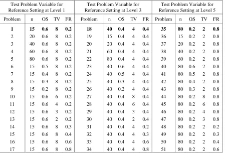
For the purpose of this experiment, every input variable is divided into five levels from low to high
difficulty values as shown in Table 1. Then a reference variable setting (datum) is selected as a baseline,
while the rest of the problem variable setting are generated by changing only one variable value at a
time. In total, there are 17 test problems (including the reference setting) generated from one reference
variable setting. In order to confirm algorithm performance, three different reference variable setting
will be used (Level 1, 3 and 5). Therefore, the complete number of test problem in this experiment is 51
problems as shown in Table 2. The bolded problem setting (Problem 1, 18 and 35) represent the
reference variable setting for Level 1, 3 and 5 respectively. The detail of the test problem is accessible
at the following link.
12
Table 1: Level of tuneable input settingLevel n OS TV FR
1 15 0.6 8 0.2
2 20 0.5 6 0.3
3 40 0.4 4 0.4
4 60 0.3 3 0.6
5 80 0.2 2 0.8
Table 2: Experimental design for mixed-model ASP and ALB
Test Problem Variable for Reference Setting at Level 1
Test Problem Variable for Reference Setting at Level 3
Test Problem Variable for Reference Setting at Level 5
Problem n OS TV FR Problem n OS TV FR Problem n OS TV FR
1 15 0.6 8 0.2 18 40 0.4 4 0.4 35 80 0.2 2 0.8
2 20 0.6 8 0.2 19 15 0.4 4 0.4 36 15 0.2 2 0.8
3 40 0.6 8 0.2 20 20 0.4 4 0.4 37 20 0.2 2 0.8 4 60 0.6 8 0.2 21 60 0.4 4 0.4 38 40 0.2 2 0.8
5 80 0.6 8 0.2 22 80 0.4 4 0.4 39 60 0.2 2 0.8 6 15 0.5 8 0.2 23 40 0.6 4 0.4 40 80 0.6 2 0.8
7 15 0.4 8 0.2 24 40 0.5 4 0.4 41 80 0.5 2 0.8 8 15 0.3 8 0.2 25 40 0.3 4 0.4 42 80 0.4 2 0.8
9 15 0.2 8 0.2 26 40 0.2 4 0.4 43 80 0.3 2 0.8 10 15 0.6 6 0.2 27 40 0.4 8 0.4 44 80 0.2 8 0.8
11 15 0.6 4 0.2 28 40 0.4 6 0.4 45 80 0.2 6 0.8 12 15 0.6 3 0.2 29 40 0.4 3 0.4 46 80 0.2 4 0.8
13 15 0.6 2 0.2 30 40 0.4 2 0.4 47 80 0.2 3 0.8 14 15 0.6 8 0.3 31 40 0.4 4 0.2 48 80 0.2 2 0.2
15 15 0.6 8 0.4 32 40 0.4 4 0.3 49 80 0.2 2 0.3 16 15 0.6 8 0.6 33 40 0.4 4 0.6 50 80 0.2 2 0.4
17 15 0.6 8 0.8 34 40 0.4 4 0.8 51 80 0.2 2 0.6
In general, the integrated ASP and ALB for single model employed three types of algorithms;
Evolutionary algorithms (including the hybridised version), Ant colony optimization (ACO) and
Discrete PSO algorithms. This work therefore will compare the MODPSO with the following algorithms
for optimization purpose:
i. Multi-Objective Genetic Algorithm (MOGA): This algorithm is one of the most frequently used
algorithms to optimise independent ASP and ALB problem, according to the survey (Rashid,
[image:13.595.71.521.232.537.2]13
ii. Ant Colony Optimisation (ACO): The ACO algorithm has been implemented for single modelintegrated ASP and ALB optimisation (Yang, Lu and Zhao, 2013; Lu and Yang, 2016).
iii. Hybrid Genetic Algorithm (HGA): The HGA that proposed by Chen is the most cited published
work on integrated ASP and ALB optimisation for single model (Chen, Lu and Yu, 2002). This
algorithm combined the heuristic approach in line balancing with Genetic Algorithm. The output
solution from the heuristic approaches will be inserted into the initial population for Genetic
Algorithm.
iv. Elitist Non-Dominated Sorting Genetic Algorithm (NSGA-II): NSGA-II was introduced by (Deb,
2002). This algorithm is selected because of its popularity in solving multi-objective optimisation.
v. Multi-Objective Particle Swarm Optimisation (MOPSO): The MOPSO algorithm introduced to
extend the PSO application for multi-objective optimisation (Coello Coello and Lechuga, 2002).
vi. Discrete Particle Swarm Optimisation (DPSO): DPSO present the discrete updating procedure to
update position and velocity (Rameshkumar, Suresh and Mohanasundaram, 2005). The discrete
representation is suitable to be used for ASP and ALB problem.
In addition to this experiment, another set of computational experiment was conducted to identify the
best coefficient values for MODPSO. There are three coefficients that influence the MODPSO
performance: inertia weight (c1), cognitive coefficient, (c2) and social coefficient (c3). In MODPSO, c1
coefficient influences the particle velocity, while c2 and c3 influence the exploring and exploiting of the
search space, respectively. The limit for these coefficients is suggested as follows: c1 [0, 1], c2 and c3 [0,
3]. In this study, a Taguchi approach with L9 orthogonal array is used. The three levels of coefficient
values are as follows::
c1 = {0.2, 0.5, 0.8}, c2 = {0.5, 1.5, 2.5} and c3 = {0.5, 1.5, 2.5}
In this experiment, 15 test problems from Table 2 are selected, which consist of 5 problems in each
14
In this work, the population or swarm size is set at 20 with 500 iterations. For each problem, 30 runswith different random seeds are performed and the output from each run are collected and filtered to
find the non-dominated solution set.
4.1 Performance indicators
To evaluate the performance of each algorithm when dealing with different complexity problems, the
following performance indicators adopted from (Deb, 2002) and (Yoosefelahi et al., 2012) are used.
i. Number of non-dominated solution in Pareto optimal, : Shows the number of non-dominated
solutions generated by each algorithm in the Pareto solution set. The higher indicates better
algorithm performance.
ii. Error Ratio, ER: ER counts the number of solutions which are not members of the Pareto optimal
set, divided by the number of solutions generated by algorithm. Smaller ER indicates better
algorithm performance.
iii. Generational Distance, GD: GD calculation yields an average distance of solution with the
nearest Pareto optimal solution. Smaller GD value indicates better algorithm performance.
iv. Spacing: This indicator measures the relative distances between each solution. Smaller Spacing
index indicates better solution set, having better spacing between each solution.
v. Maximum Spread, Spreadmax: Measures the spread of solutions found by each algorithm. Larger
maximum spread is the better.
5. Results of Computational Experiment
Due to the large size data from the optimization, the results were simplified the data by using standard
competition rank approach. The best algorithm for a particular indicator and test problem was assigned
rank 1 while the worst was assigned as rank 7. When the algorithm performance is a tie, an equal rank
will be assigned and the next rank will be left empty. Table 3 present the frequency of the rank obtained
15
optimal ( ) indicator, the MODPSO comes out with better solution sets in 96% of test problems, whilethe remaining 4% belong to NSGA-II. The Error Ratio (ER) indicator also shows that the leading
algorithms are MODPSO and NSGA-II. The MODPSO and NSGA-II show better performance in 41.5%
and 58.5% respectively. Both algorithms also dominate the best performance for Generational Distance
(GD) indicator with 43% of better performance for MODPSO and 53% for NSGA-II. Meanwhile, the
Spacing indicator shows different pattern, where the largest percentages of better performance are
MOPSO (22), followed by HGA (20%), ACO (19%), DPSO (17%), MOGA (14%), MODPSO (6%)
and NSGA-II (2%). On the other hand, the Spreadmax indicator that measure the extent of solution
distribution presents that the MODPSO algorithm produce better solution in 70% of the problem. The
MOPSO perform better in 18%, while the remaining balances are shared among DPSO (6%), MOGA
[image:16.595.72.487.386.763.2](4%) and HGA (2%).
Table 3: Frequency of the rank obtained by each algorithm
Indicator Rank MOGA ACO HGA NSGA-II MOPSO DPSO MODPSO
1 0 0 0 5 0 0 47
2 0 1 8 37 1 0 4
3 11 2 22 5 12 8 0
4 15 10 8 3 18 11 0
5 12 5 8 1 11 14 0
6 8 8 4 0 6 18 0
7 5 25 1 0 3 0 0
ER
1 0 0 0 31 0 0 23
2 0 0 5 17 1 0 26
3 10 6 20 3 4 5 2
4 19 8 11 0 18 7 0
5 8 5 11 0 13 16 0
6 10 9 4 0 11 19 0
7 4 23 0 0 4 4 0
GD
1 0 0 0 30 0 0 24
2 2 0 6 17 1 0 22
3 17 3 23 2 2 1 3
4 20 6 10 1 7 6 1
5 8 7 8 0 17 10 1
6 3 5 3 1 19 21 0
7 1 30 1 0 5 13 0
Spacing
1 7 8 7 8 13 5 3
2 10 2 4 10 10 6 9
3 11 7 6 7 13 5 2
4 1 3 4 5 4 14 20
5 10 13 10 6 7 3 2
6 9 11 13 10 2 4 2
16
Spreadmax1 2 1 1 0 10 4 33
2 3 1 8 2 16 15 7
3 5 2 14 4 11 12 2
4 7 3 12 7 8 12 2
5 13 6 11 6 5 5 5
6 13 15 3 16 1 2 1
[image:17.595.71.487.69.161.2]7 8 23 2 16 0 1 1
Table 4 presents the mean of performance indicators for all test problems. Based on the mean values,
the best performance of indicator is observed in MODPSO and the followed by NSGA-II algorithms.
Meanwhile, the best mean performance for ER and GD indicators is achieved by NSGA-II, while the
MODPSO in second place. In the meantime, two PSO-based algorithms, MOPSO and DPSO are leading
the mean of Spacing indicator. Furthermore, the PSO-based algorithms also show better performance
[image:17.595.70.497.364.488.2]compared with other algorithms in Spreadmax indicator.
Table 4: Mean of performance indicators
Indicator Algorithm
MOGA ACO HGA NSGA-II MOPSO DPSO MODPSO
1 4.7843 1.9020 8.0588 27.2353 5.2745 3.4902 41.0196
ER2 0.9037 0.9632 0.8592 0.1952 0.9230 0.9444 0.2046
GD2 1.9951 2.4650 2.0017 0.1753 2.3219 2.3682 0.2696
Spacing2 1.0281 1.1410 0.9819 1.2898 0.9479 0.9537 1.2318
Spreadmax1 15.7278 14.6364 16.5250 14.9729 17.1868 16.8720 18.4656
[image:17.595.74.484.549.656.2]1 Larger the better indicator 2 Smaller the better indicator
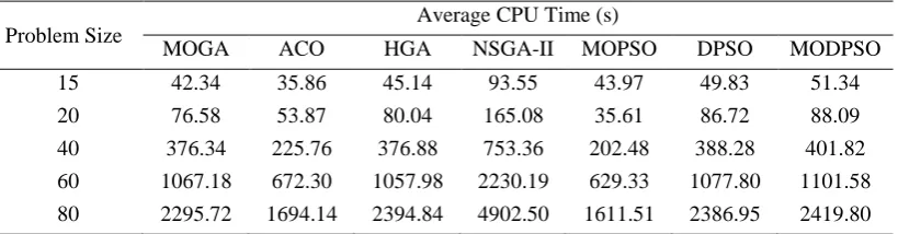
Table 5: Average CPU time for different problem size
Problem Size
Average CPU Time (s)
MOGA ACO HGA NSGA-II MOPSO DPSO MODPSO
15 42.34 35.86 45.14 93.55 43.97 49.83 51.34 20 76.58 53.87 80.04 165.08 35.61 86.72 88.09
40 376.34 225.76 376.88 753.36 202.48 388.28 401.82 60 1067.18 672.30 1057.98 2230.19 629.33 1077.80 1101.58
80 2295.72 1694.14 2394.84 4902.50 1611.51 2386.95 2419.80
Table 5 shows the average CPU time for different problem size. In general, the ACO and MOPSO were
among the fastest algorithm to complete the iteration. Meanwhile, the MODPSO was roughly in the
second last position, in front of NSGA-II in term of CPU time. For comparison, the MODPSO was just
17
procedures compared with regular updating procedures in MOPSO. However, the NSGA-II requiredmostly double CPU time compared with MODPSO. This is because the NSGA-II combined the existing
population and new offspring for the non-dominated sorting procedure. Therefore, the time taken to
complete the iteration was increased compared with other algorithms.
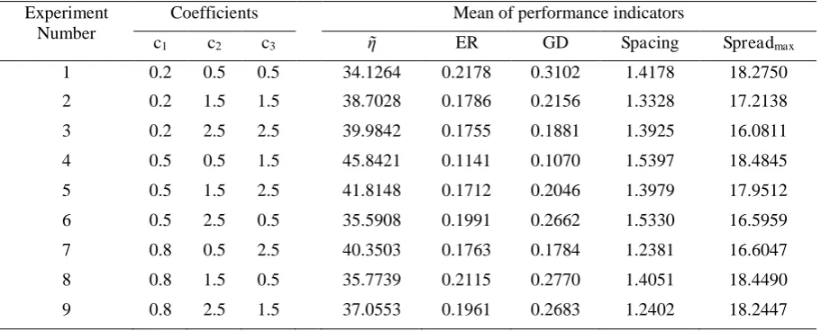
[image:18.595.71.527.386.570.2]5.1 MODPSO Coefficient Tuning
Table 6 shows the results of the MODPSO coefficient experiment. The experimental table was designed
using Taguchi L9 orthogonal array. Based on the general observation, experiment number 4 led in term
of the best solution of cardinality, which was represented by and ER. The same experiment also came
out with the best accuracy (i.e. GD indicator).
Table 6: MODPSO coefficient experiment results
Experiment Number
Coefficients Mean of performance indicators
c1 c2 c3 ER GD Spacing Spreadmax
1 0.2 0.5 0.5 34.1264 0.2178 0.3102 1.4178 18.2750
2 0.2 1.5 1.5 38.7028 0.1786 0.2156 1.3328 17.2138
3 0.2 2.5 2.5 39.9842 0.1755 0.1881 1.3925 16.0811
4 0.5 0.5 1.5 45.8421 0.1141 0.1070 1.5397 18.4845
5 0.5 1.5 2.5 41.8148 0.1712 0.2046 1.3979 17.9512
6 0.5 2.5 0.5 35.5908 0.1991 0.2662 1.5330 16.5959
7 0.8 0.5 2.5 40.3503 0.1763 0.1784 1.2381 16.6047
8 0.8 1.5 0.5 35.7739 0.2115 0.2770 1.4051 18.4490
9 0.8 2.5 1.5 37.0553 0.1961 0.2683 1.2402 18.2447
Meanwhile, Figure 4 presents the main effect plots of c1, c2 and c3 for different performance indicators.
Based on the main effect plots, medium c1, low c2 and medium c3 coefficients were preferable as
observed in and ER plots to produce a solution with good cardinality. Similar coefficients’ levels were
also required to generate accurate solutions as represented by the GD indicator. On the other hand, the
main effect plots by Spacing and Spreadmax indicated that high c1, medium c2 and medium c3
18
[Figure 4: Effect of w, c1 and c2 on Performance Indicators: (a) , (b) ER, (c) GD, (d) Spacing, and (e)Spreadmax]
6. Discussion of Results
In general, the result from experiment shows that the performance of algorithms in optimising integrated
mixed-model ASP and ALB appear to be dominated by NSGA-II and proposed MODPSO algorithms,
especially in four performance indicators (i.e. , ER, GD and Spreadmax). However further analyses are
required to quantify the results. Therefore, a statistical test is conducted to measure the significance of
the improvements achieved by the MODPSO in optimising integrated mixed-model ASP and ALB.
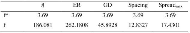
The Analysis of Variance (ANOVA) test was then carried out to evaluate any significant improvement
between the results obtained by different algorithms. The ‘null hypothesis’ stated that there is no
significant improvement among the means of all algorithm results. The alternative hypothesis state that
there is significant improvement among means in the result of at least one algorithm. The null hypothesis
will be accepted when the calculated value is smaller than critical value (f*) as suggested in the
[image:19.595.70.387.563.618.2]f-distribution table (Coolidge, 2000). The result of ANOVA test is presented in Table 7.
Table 7: Summary of ANOVA test
ER GD Spacing Spreadmax
f* 3.69 3.69 3.69 3.69 3.69
f 186.081 262.1808 45.8928 12.8327 17.4301
f*: critical f-value f: calculated f-value
The result shows that the calculated f-value for all performance indicators are consistently larger than f*
at 0.05 confidence interval. Therefore, the null hypothesis is rejected and the alternative is accepted for
19
indicators in at least one algorithm. However, the ANOVA test cannot differentiate the exactimprovement of one algorithm in comparison with another algorithm.
Therefore a posteriori test known as Tukey’s Honestly Significant Difference (HSD) is performed. This
test is performed by calculating the absolute mean difference between the results of one algorithm over
another algorithm, which is then compared with the critical HSD (HSD*) value. The HSD* value for
algorithm i is calculated as follows.
HSD Eq. 11
The q value is acquired from Tukey’s table, MSW is the mean squares within groups from ANOVA
test, and n is the number of data in each group. When the absolute mean difference is larger than HSD*,
a significant improvement has been identified in one algorithm over another algorithm. At this point,
we are interested to know the performance of MODPSO over the other algorithms. Table 8 presents the
[image:20.595.70.473.475.650.2]HSD* and absolute mean difference between MODPSO and the other algorithms.
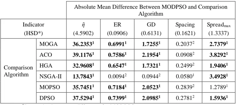
Table 8: Summary of Tukey’s HSD test for MODPSO algorithm
Absolute Mean Difference Between MODPSO and Comparison Algorithm
Indicator
(HSD*) (4.5902)
ER (0.0906)
GD (0.6131)
Spacing (0.1621)
Spreadmax (1.3337)
Comparison Algorithm
MOGA 36.23531 0.69911 1.72551 0.20372 2.73791
ACO 39.11761 0.75861 2.19541 0.09082 3.82921
HGA 32.96081 0.65471 1.73211 0.24992 1.94061
NSGA-II 13.78431 0.00942 0.09442 0.05801 3.49281
MOPSO 35.74511 0.71841 2.05231 0.28392 1.27891
DPSO 37.52941 0.73991 2.09851 0.27812 1.59361 1Better absolute mean difference for MODPSO
2Better absolute mean difference for comparison algorithm
In Table 8, the values that are labelled ‘1’ show the MODPSO has a better mean difference over the
comparison algorithm, while the values labelled ‘2’ mean that the comparison algorithm has a better
20
improvements achieved by MODPSO over other algorithms, since the absolute mean difference is largerthan HSD*. Based on Table 8, the MODPSO algorithm shows better performance and significant
improvement when compared with the set of algorithms for indicator. The MODPSO also show
significant improvements for ER and GD indicators compared with other algorithms, with the exception
of NSGA-II. In both indicators, the NSGA-II algorithm shows better mean difference compare with
MODPSO, however, the difference is not significant because the absolute mean difference are smaller
than HSD*.
Meanwhile, the Spacing indicator did not show any significant improvement of MODPSO although it
has a better mean difference when compared with NSGA-II. Except for NSGA-II, all other algorithms
show better performance over MODPSO, where significant improvements are presented by four
algorithms (MOGA, HGA, MOPSO and DPSO). For Spreadmax indicator, the MODPSO algorithm
shows significant improvement compared with other algorithms, except MOPSO. In comparison with
MOPSO, although no significant improvement is achieved, the MODPSO algorithm still produces better
solution.
In this work, the solution quality towards Pareto optimal are measured using three performance
indicators i.e. , ER and GD. The Spacing indicator measures the uniformity of the found solutions and
Spreadmax measures the ability of algorithm to explore the extreme solutions within the solution space.
The results from statistical test explain that, the MODPSO algorithm shows significant improvement in
term of finding better solution towards Pareto optimal over comparison algorithms, with the exception
of NSGA-II at 0.05 confidence intervals.
Furthermore, the Spreadmax result means that the MODPSO algorithm is significantly able to explore
better extreme solutions when compared with MOGA, ACO, HGA, DPSO and NSGA-II. Meanwhile,
in term of uniformity of solution spread, the MODPSO algorithm did not perform significantly better
than other algorithms. The Spacing indicator considers all non-dominated solutions that was found by a
21
space, the algorithm that generated more non-dominated solutions has greater chances to produce betterSpacing. From the experiment, the mean number of non-dominated solutions generated by the
algorithms (regardless of Pareto or non-Pareto optimal), in ascending order, are: NSGA-II (33.84), ACO
(46.9), MODPSO (55.37), MOGA (56.14), HGA (68.91), DPSO (80.47) and MOPSO (85.02). These
numbers clearly present the algorithms that show significant improvement over MODSPO for Spacing
indicator are the algorithms with larger mean of generated solutions.
The result from experiments and statistical tests summarise that the MODPSO has shown significant
improvement over the majority of compared algorithms in , ER, GD and Spreadmax indicators. In
comparison with all other algorithms, the performance of MODPSO is closely followed by NSGA-II,
where the MODPSO only show significant improvement over NSGA-II in and Spreadmax indicators.
In order to compare performance of NSGA-II, the mean difference between NSGA-II and other
[image:22.595.73.478.480.621.2]algorithms are calculated and presented in Table 9.
Table 9: Summary of Tukey’s HSD test for NSGA-II
Absolute Mean Difference Between NSGA-II and Comparison Algorithm
Indicator
(HSD*) (4.5902)
ER (0.0906)
GD (0.6131)
Spacing (0.1621)
Spreadmax (1.3337)
Comparison Algorithm
MOGA 22.45101 0.70851 1.81991 0.26182 0.75492
ACO 25.33331 0.76801 2.28971 0.14892 0.33651
HGA 19.17651 0.66401 1.82641 0.30792 1.55222
MOPSO 21.96081 0.72781 2.14661 0.34192 2.21392
DPSO 23.74511 0.74921 2.19291 0.33612 1.89912
MODPSO 13.78432 0.00941 0.09441 0.05802 3.49282 1Better absolute mean difference for NSGA-II
2Better absolute mean difference for comparison algorithm
Table 9 indicates that the NSGA-II has significant improvement for solution quality leading to Pareto
optimal compared with other algorithms except the MODPSO. Besides that, the NSGA-II did not show
any significant improvement for solution uniformity (Spacing) and extreme solution exploration
22
(Table 9) over other algorithms, the MODPSO is found to perform better than NSGA-II. This is becausethe MODPSO have shown significant improvement over NSGA-II in two of indicators (i.e. and
Spreadmax), while there is no significant improvement of NSGA-II over MODPSO algorithm.
Furthermore, for Spreadmax indicator, the NSGA-II did not show any significant improvement as
MODPSO shows when compared with all other algorithms. In addition, the NSGA-II required double
CPU time to complete the iteration compared with MODPSO as presented in Table 5. These facts give
more advantages to MODPSO in term of solution quality and also algorithm effort.
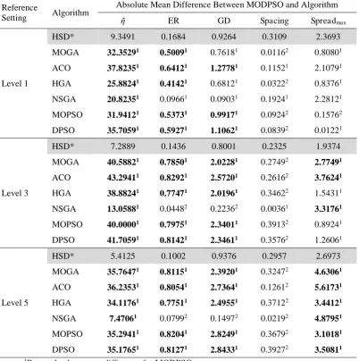
The result from Tukey’s HSD test for integrated mixed-model ASP and ALB clearly shows that the
MODPSO performed better than other algorithms for all test problems. Another question that arises is
the problem category that the MODPSO algorithm performed best and worst. Therefore, the Tukey’s
HSD test based on different problem reference setting is conducted. The result of Tukey’s HSD test for
different problem setting is presented in Table 10. Based on Table 10, the MODPSO shows significant
improvement in indicator over all algorithms for all reference setting. For ER indicator, the MODPSO
consistently demonstrates significant improvement over other algorithms except NSGA-II. Meanwhile
for GD indicator in low level reference setting (Level 1), significant improvements for MODPSO are
only found over ACO, MOPSO and DPSO algorithms. However, when the reference setting is changed
to medium (Level 3) and high (Level 5) levels, significant improvements are also observed in
comparison with MOGA and NSGA-II.
On the other hand, the MODPSO consistently did not show any significant improvement over any
algorithm for Spacing indicator. For Spreadmax indicator, the proposed algorithm also did not show
significant improvements in low level reference setting. However, when the reference setting is moved
to medium level, the MODPSO shows significant improvement over MOGA, ACO and NSGA-II.
Finally, in the problem with high level reference setting, significant improvements are achieved by
MODPSO over all other algorithms. From this result, the best performance of MODPSO is found in the
23
level reference setting, even though the overall performance in this problem category is still better than [image:24.595.80.483.227.632.2]other algorithms.
Table 10: Summary of Tukey’s HSD test for MODPSO by reference setting level
Reference
Setting Algorithm
Absolute Mean Difference Between MODPSO and Algorithm
ER GD Spacing Spreadmax
Level 1
HSD* 9.3491 0.1684 0.9264 0.3109 2.3693
MOGA 32.35291 0.50091 0.76181 0.01162 0.80801
ACO 37.82351 0.64121 1.27781 0.11521 2.10791
HGA 25.88241 0.41421 0.68121 0.03222 0.83761
NSGA 20.82351 0.09661 0.09031 0.19241 2.28121
MOPSO 31.94121 0.53731 0.99171 0.09242 0.15762
DPSO 35.70591 0.59271 1.10621 0.08392 0.01221
Level 3
HSD* 7.2889 0.1436 0.8001 0.2325 1.9374
MOGA 40.58821 0.78501 2.02281 0.27492 2.77491
ACO 43.29411 0.82921 2.57201 0.26162 3.76241
HGA 38.88241 0.77471 2.01961 0.34622 1.54311
NSGA 13.05881 0.04482 0.22362 0.00361 3.31761
MOPSO 40.00001 0.79751 2.34011 0.39132 0.89241
DPSO 41.70591 0.81421 2.34611 0.35762 1.26061
Level 5
HSD* 5.4125 0.1002 0.9376 0.2957 2.6973
MOGA 35.76471 0.81151 2.39201 0.32472 4.63061
ACO 36.23531 0.80541 2.73641 0.12612 5.61731
HGA 34.11761 0.77511 2.49551 0.37122 3.44121
NSGA 7.47061 0.07992 0.14972 0.02192 4.87951
MOPSO 35.29411 0.82041 2.82491 0.36792 3.10181
DPSO 35.17651 0.81271 2.84331 0.39272 3.50811 1Better absolute mean difference for MODPSO
2Better absolute mean difference for comparison algorithm
The performance of MODPSO in optimising integrated mixed-model ASP and ALB because this
algorithm was specifically developed for discrete multi-objective optimisation problem. This algorithm
use similar procedure for Initialisation, Evaluation and Selection strategies as in II. The
24
performed well in this application. However, it does not have the fine tuning feature. The fine tuningfeature means ability of algorithm to make small adjustments to solution in order to achieve the best or
a desired performance. This is an important feature for ASP and ALB, where small changes may lead
to sudden improvement in results.
The discrete updating procedure in MODPSO is designed to enable fine tuning towards the end of
iterations. According to discrete updating procedure (Subtraction operator (Xi-Xj)) in Section 3.4, zero
velocity is given when similar element in Xi and Xj is found (this is the case when all particles move
towards the best solution at the end of iterations). When majority of velocity elements are zero, only
small changes occur in assembly sequence as presented by Addition operator (Xi+Vi) in Section 3.4. This
feature allows fine tuning of the assembly sequences in MODPSO.
7. Conclusions
This paper formulates and studies the optimisation of integrated mixed-model Assembly Sequence
Planning (ASP) and Assembly Line Balancing (ALB) problem using Multi-objective Discrete Particle
Swarm Optimisation (MODPSO). A set of test problems with different range of difficulties has been
used to test the performance of MODPSO in optimising integrated mixed-model ASP and ALB. In
addition, MODPSO coefficient tuning has been conducted to identify the best settings for optimisation.
The experimental results indicate that, in general, the MODPSO algorithms performed better than other
comparison algorithms. Statistical test concluded that the MODPSO has shown significant improvement
in converging to Pareto optimal solution and exploring the extreme solutions in search space. The
statistical test also concluded that the MODPSO performed best in the problem with high level of
difficulty. Meanwhile the weakest performance is in the problem at low difficulty level, although it still
25
optimum performance for solution cardinality and accuracy was achieved when the inertia weight andsocial coefficient were at the medium level, while cognitive coefficient was at the low level.
The work in this paper has initiates the study on integrated mixed-model ASP and ALB optimisation.
At the same time, it also indicates that the MODPSO algorithm is able to optimise this problem better
than comparison algorithms. One of the MODPSO’s downside is incapability of generating uniformly
spaced solutions as presented by Spacing indicator. In future, an effort to improve the algorithm
performance, especially in solution uniformity is proposed to improve overall solution quality. The first
suggestions to improve solution uniformity is to consider the historical data in the crowding distance.
This will make the unselected solutions because of mating pool capacity, will be taken into account
when calculating the crowding distance. Besides that, the solution quality also could be improved by
including the extreme solutions as a part of MODPSO updating procedure. It will influence the
MODPSO convergence direction towards the extreme solution, besides the Gbest. Therefore, the search
direction become more diverse.
Funding: This work was supported by Universiti Malaysia Pahang under grant RDU180331.
Conflict of Interest: The authors declare that they have no conflict of interest.
References
Ab. Rashid, M. F. F. (2013) Integrated Multi-Objective Optimisation of Assembly Sequence Planning and Assembly Line Balancing using Particle Swarm Optimisation, PhD Thesis, Cranfield University.
Ab. Rashid, M. F. F., Tiwari, A. and Hutabarat, W. (2017) ‘Comparison of Sequential and Integrated
Optimisation Approaches for ASP and ALB’, Procedia CIRP. The Author(s), 63, pp. 505–510. doi: 10.1016/j.procir.2017.03.083.
Ab Rashid, M. F. F., Hutabarat, W. and Tiwari, A. (2012) ‘Development of a tuneable test problem
generator for assembly sequence planning and assembly line balancing’, Proceedings of the Institution of Mechanical Engineers, Part B: Journal of Engineering Manufacture, 226(11), pp. 1900–1913. doi: 10.1177/0954405412457621.
26
balancing’, European Journal of Operational Research, 168(3), pp. 694–715. doi:
10.1016/j.ejor.2004.07.023.
Buyukozkan, K. et al. (2016) ‘Lexicographic bottleneck mixed-model assembly line balancing
problem: Artificial bee colony and tabu search approaches with optimised parameters’, Expert Systems
with Applications, 50, pp. 151–166. doi: http://dx.doi.org/10.1016/j.eswa.2015.12.018.
Chen, R., Lu, K. and Yu, S. (2002) ‘A hybrid genetic algorithm approach on multi-objective of
assembly planning problem’, Engineering Applications of Artificial Intelligence, 15(2002), pp. 447–
457.
Coello Coello, C. A. and Lechuga, M. S. (2002) ‘MOPSO: a proposal for multiple objective particle
swarm optimization’, in Proceedings of the 2002 Congress on Evolutionary Computation. CEC’02
(Cat. No.02TH8600). IEEE, pp. 1051–1056. doi: 10.1109/CEC.2002.1004388.
Coolidge, F. L. (2000) Statistics: A Gentle Introduction. London: SAGE Publication.
Deb, K. (2002) Multi-Objective Optimization using Evolutionary Algorithms. Sussex, United Kingdom: John Wiley & Sons.
Hu, S. J. et al. (2008) ‘Product variety and manufacturing complexity in assembly systems and supply
chains’, {CIRP} Annals - Manufacturing Technology, 57(1), pp. 45–48. doi:
http://dx.doi.org/10.1016/j.cirp.2008.03.138.
Hu, Y.-J. et al. (2014) ‘Machining scheme selection based on a new discrete particle swarm
optimization and analytic hierarchy process’, Artificial Intelligence for Engineering Design, Analysis
and Manufacturing. Cambridge University Press, 28(1), pp. 71–82. doi: 10.1017/S0890060413000504.
Jusop, M. and Ab Rashid, M. F. F. (2015) ‘A review on simple assembly line balancing type-e
problem’, IOP Conference Series: Materials Science and Engineering, 100, p. 12005. doi:
10.1088/1757-899X/100/1/012005.
Kara, Y. et al. (2011) ‘Multi-objective approaches to balance mixed-model assembly lines for model
mixes having precedence conflicts and duplicable common tasks’, The International Journal of
Advanced Manufacturing Technology, 52(5), pp. 725–737. doi: 10.1007/s00170-010-2779-z.
Lin, M.-C. et al. (2012) ‘A modularized contact-rule reasoning approach to the assembly sequence
generation for product design’, Concurrent Engineering, 20(3), pp. 203–221. doi:
10.1177/1063293X12452419.
Lu, C. and Yang, Z. (2016) ‘Integrated assembly sequence planning and assembly line balancing with
ant colony optimization approach’, The International Journal of Advanced Manufacturing
Technology. Springer London, 83(1), pp. 243–256. doi: 10.1007/s00170-015-7547-7.
27
South Australia.Mirabi, M. (2015) ‘A novel hybrid genetic algorithm for the multidepot periodic vehicle routing
problem’, Artificial Intelligence for Engineering Design, Analysis and Manufacturing, 29(1), pp. 45–
54. doi: 10.1017/S0890060414000328.
Penciuc, D. et al. (2016) ‘Product life cycle management approach for integration of engineering design and life cycle engineering’, Artificial Intelligence for Engineering Design, Analysis and Manufacturing, 30(4), pp. 379–389. doi: 10.1017/S0890060416000366.
Rahman, H. F., Sarker, R. and Essam, D. (2017) ‘A genetic algorithm for permutation flowshop
scheduling under practical make-to-order production system’, Artificial Intelligence for Engineering Design, Analysis and Manufacturing, 31(1), pp. 87–103. doi: 10.1017/S0890060416000196.
Rameshkumar, K., Suresh, R. K. and Mohanasundaram, K. M. (2005) ‘Discrete Particle Swarm
Optimization ( DPSO ) Algorithm for Permutation Flowshop Scheduling to Minimize Makespan’,
Advances in Natural Computation, 3612, pp. 572–581.
Rashid, M. F. F., Hutabarat, W. and Tiwari, A. (2011) ‘A review on assembly sequence planning and
assembly line balancing optimisation using soft computing approaches’, The International Journal of
Advanced Manufacturing Technology, 59(1–4), pp. 335–349. doi: 10.1007/s00170-011-3499-8.
Roshani, A. and Nezami, F. G. (2017) ‘Mixed-model multi-manned assembly line balancing problem:
A mathematical model and a simulated annealing approach’, Assembly Automation, 37(1), pp. 34–50.
doi: 10.1108/AA-02-2016-016.
Shankar, P., Summers, J. D. and Phelan, K. (2017) ‘A verification and validation planning method to
address change propagation effects in engineering design and manufacturing’, Concurrent
Engineering, 25(2), pp. 151–162. doi: 10.1177/1063293X16671771.
Tasan, S. O. and Tunali, S. (2008) ‘A review of the current applications of genetic algorithms in
assembly line balancing’, Journal of Intelligent Manufacturing, 19(1), pp. 49–69. doi:
10.1007/s10845-007-0045-5.
Tseng, H.-E. et al. (2008) ‘Hybrid evolutionary multi-objective algorithms for integrating assembly
sequence planning and assembly line balancing’, International Journal of Production Research,
46(21), pp. 5951–5977. doi: 10.1080/00207540701362564.
Tseng, H.-E. and Tang, C.-E. (2006) ‘A sequential consideration for assembly sequence planning and
assembly line balancing using the connector concept’, International Journal of Production Research,
44(1), pp. 97–116. doi: 10.1080/00207540500250606.
Yang, Z., Lu, C. and Zhao, H. W. (2013) ‘An Ant Colony Algorithm for Integrating Assembly
28
Yoosefelahi, A. et al. (2012) ‘Type II robotic assembly line balancing problem: An evolutionstrategies algorithm for a multi-objective model’, Journal of Manufacturing Systems, 31(2), pp. 139– 151. doi: 10.1016/j.jmsy.2011.10.002.
Zeng, K. et al. (2014) ‘Probability increment based swarm optimization for combinatorial
optimization with application to printed circuit board assembly’, Artificial Intelligence for Engineering Design, Analysis and Manufacturing. Cambridge University Press, 28(4), pp. 429–437. doi:
10.1017/S0890060413000632.
Zhong, Y. (2017) ‘Hull mixed-model assembly line balancing using a multi-objective genetic
algorithm simulated annealing optimization approach’, Concurrent Engineering, 25(1), pp. 30–40.
doi: 10.1177/1063293X16666204.
Zhu, X. et al. (2012) ‘A complexity model for sequence planning in mixed-model assembly lines’, Journal of Manufacturing Systems, 31(2), pp. 121–130. doi: