Proc IMechE Part B: J Engineering Manufacture 1–16
ÓIMechE 2016 Reprints and permissions:
sagepub.co.uk/journalsPermissions.nav DOI: 10.1177/0954405416673095 pib.sagepub.com
Multi-objective discrete particle swarm
optimisation algorithm for integrated
assembly sequence planning and
assembly line balancing
Mohd Fadzil Faisae Ab Rashid
1,2, Windo Hutabarat
1and Ashutosh Tiwari
1Abstract
In assembly optimisation, assembly sequence planning and assembly line balancing have been extensively studied because both activities are directly linked with assembly efficiency that influences the final assembly costs. Both activities are cate-gorised as NP-hard and usually performed separately. Assembly sequence planning and assembly line balancing optimisa-tion presents a good opportunity to be integrated, considering the benefits such as larger search space that leads to better solution quality, reduces error rate in planning and speeds up time-to-market for a product. In order to optimise an integrated assembly sequence planning and assembly line balancing, this work proposes a multi-objective discrete par-ticle swarm optimisation algorithm that used discrete procedures to update its position and velocity in finding Pareto optimal solution. A computational experiment with 51 test problems at different difficulty levels was used to test the multi-objective discrete particle swarm optimisation performance compared with the existing algorithms. A statistical test of the algorithm performance indicates that the proposed multi-objective discrete particle swarm optimisation algo-rithm presents significant improvement in terms of the quality of the solution set towards the Pareto optimal set.
Keywords
Integrated assembly sequence planning and assembly line balancing, particle swarm optimisation, multi-objective optimi-sation, discrete particle swarm optimisation
Date received: 10 November 2015; accepted: 14 September 2016
Introduction
In the recent years, various multi-objective optimisation techniques have been proposed to solve assembly
opti-misation problems.1–3 This trend shows the attention
given by researchers to assembly optimisation activities because of their complexity and relevance of the actual industrial problems. The research in assembly optimisa-tion can be classified according to product development
and production stage.4Although there are many
activi-ties classified in the assembly optimisation, assembly sequence planning (ASP) and assembly line balancing (ALB) are the most prominent because they are directly linked with assembly efficiency.
ASP refers to a task for which planners, usually based on their particular heuristics in assembling all the components of a product, arrange a specific collision-free assembly sequence according to the product design
description.5,6Figure 1 shows a common assembly
rep-resentation using a precedence graph. From this graph, numerous feasible assembly sequences can be generated
such as {1 6 7 2 4 3 5}, {1 7 3 6 5 4 2} or {1 6 2 7 4 3 5}. Based on this example, ASP is about determining the most optimum sequence to assemble a product from all feasible assembly sequences.
Once the optimum assembly sequence has been determined from ASP activity, the assembly jobs will be assigned to workstations, so that every workstation will have equal or almost equal workload. The assem-bly job assignment activity refers to ALB that is defined as the decision problem of optimally partitioning assembly work among stations with respect to some
1Manufacturing and Materials Department, Cranfield University,
Cranfield, UK
2Faculty of Mechanical Engineering, University Malaysia Pahang, Pahang,
Malaysia
Corresponding author:
Mohd Fadzil Faisae Ab Rashid, Manufacturing and Materials Department, Cranfield University, Cranfield MK43 0AL, UK.
objectives and constraints.7,8For example, let the opti-mum assembly sequence from ASP be {1 6 2 7 4 3 5} and this assembly jobs will be assigned to three work-stations. There are many possible assembly job assign-ment combinations such as {(1 6), (2 7 4), (3 5)} or {(1 6 2), (7 4), (3 5)} or {(1 6 2 7), (4 3), (5)}. In this pro-cess, ALB will determine the best assembly job combi-nation which comes out with equal or almost equal workload between workstations.
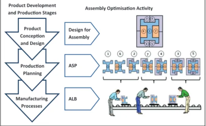
Figure 2 shows the main assembly optimisation activities in every product development and production stage. Based on this figure, ASP and ALB activities are performed individually because they take place in dif-ferent stages of the product development process. ASP is located in the production planning while ALB is in
the manufacturing process stage.4However, the current
global market drives a demand for shorter product life-cycles and also for products to be more competitive in terms of time-to-market, quality and also manufactur-ing cost. One approach to stay competitive is by inte-grating manufacturing activities across the different
stages.9From the aspect of assembly optimisation, the
ASP and ALB optimisation activities present a good integration opportunity with various potential benefits to the manufacturer.
The main benefit of using an integrated ASP and ALB is that the quality of assembly plans could be improved as the search space of the integrated problem
would become larger than when optimising each prob-lem sequentially. Besides, the integrated ASP and ALB could reduce the rate of errors in both planning and
costing during the manufacturing stages.5At the same
time, the integrated optimisation also speeds up the aspect of time-to-market for a product.
In ASP and ALB optimisation, several objectives have been used to determine the optimal solution for the problem. When an optimisation problem involves more than one objective, this problem is known as
multi-objective optimisation.10 Traditionally, the
sim-plest way to optimise multi-objective problem is to bundle all the objectives into a single fitness using some kind of weighted assignment. However, this approach requires high prior knowledge on the importance of one objective over another. Therefore, instead of focus-ing on one sfocus-ingle optimum point, the researchers might be interested in all the best options available, which are
known as Pareto optimal solutions.11Furthermore, by
having a set of optimum solutions, the decision-makers in the industry are offered more flexibility in selecting the solution that is deemed suitable with a variety of preferences.
Although various optimisation algorithms have been developed and used to optimise different multi-objective problems, to the best of the authors’ knowl-edge, only techniques based on genetic algorithm (GA) and ant colony optimisation (ACO) have been
pro-posed to optimise integrated ASP and ALB.1,12,13Chen
et al.14 proposed a hybrid GA to optimise integrated
ASP and ALB, where GA is combined with heuristic search. The objectives were to minimise cycle time, maximise workload smoothness, minimise tool changes, minimise the number of tools and minimise the total penalty of assembly relations. Although this article does not clearly state the integration of ASP and ALB, this relationship was acknowledged following the optimisa-tion objectives.
Tseng and Tang studied combining ASP together with ALB based on the assembly ‘connectors’ (i.e. the connector basis) using GA. In their work, optimisation was conducted in three stages. First, each part was assigned to a specific connector type. Then, the algo-rithm generated the assembly planning based on the connectors. Finally, the algorithm assigned the connec-tors to stations and selected proper types of stations. Meanwhile, in the second and third stages, GA was applied to generate connector-based assembly in a sequential order, as well as to determine the suitable station types for the sequential order. However, when using this approach, whenever the number of connec-tors is increased, a few of the parameters that govern
GA performance need to be reset.5
Another work by Tseng et al.15 on integrated ASP
and ALB was done in 2008. This work adopted the
hybrid evolutionary multi-objective algorithm
(HEMOA) that was based on GA. On the basis of
multi-objective optimisation, the Pareto optimal
approach was adopted in this study. However, the
Figure 2. Main assembly optimisation activities in product development and production stages.
weighted sum approach was employed to obtain a better solution, instead of measuring the solution crowding that has been frequently used in recent multi-objective algorithm.
Another integrated ASP and ALB optimisation work was also formulated based on the assembly
con-nectors.16 In this work, the guided-modified weighted
Pareto-based multi-objective genetic algorithm (G-WPMOGA) had been proposed to optimise the inte-grated ASP and ALB problem with two, three and four objectives. The proposed algorithm displayed better performance in the problem with two and four objec-tives, but not in the problem with three objectives.
In the recent optimisation work of integrated ASP and ALB, the GA-based algorithms performed well in optimising the problem with low and medium difficul-ties. However, the performance of GA-based algo-rithms did not last when optimising high difficulty problem, especially the problem with a large number of
tasks.17 On the other hand, the researcher also
con-cluded that the different GA-based variants should be used in order to optimise the problem with a different
number of criteria.16
Besides GA-based algorithm, the researcher imple-mented ant colony algorithm to optimise the integrated
ASP and ALB problems.12,13In Yang et al.,12they
pro-posed an optimisation model to implement ACO for integrated ASP and ALB without numerical
experi-ment. Meanwhile, in Lu and Yang,13the authors
opti-mised several objectives such as line efficiency, smoothness index, assembly time and number of work-stations. However, the problem was treated as single objective, by combining all the objectives. In order to overcome the limitation, a new algorithm to optimise integrated ASP and ALB problems is needed.
In many different works that compare algorithm performance, particle swarm optimisation (PSO) has shown strong performance compared with competing algorithms. This algorithm is popular due to its simpli-city and ability to quickly converge to a reasonably
good solution.18 PSO is a population-based stochastic
optimisation technique that was developed by Kennedy and Eberhart in 1995. In PSO, the potential solutions, called particles, ‘fly’ through the problem space by
fol-lowing the current optimum particles.19In micro-ASP,
PSO was found to provide less computational time
compared with other considered algorithms.20PSO was
shown to outperform GA and simulated annealing in scheduling problems in the majority of applications by considering computation efficiency, optimality and
robustness.21 In another research, PSO was found to
perform better than GA, memetic algorithm, shuffled frog leaping and ant algorithm in solving continuous
and discrete optimisation problems.22 PSO algorithm
also performs better compared with commercial
soft-ware for robotic ALB problem.23
Even though several researches on ASP and ALB
implemented PSO, they were independent works.24–27
At this point, no existing works are using PSO
algorithms to optimise the integrated ASP and ALB problems. In this article, the multi-objective discrete particle swarm optimisation (MODPSO) to optimise integrated ASP and ALB is proposed. In comparison
with Nearchou,28 Coello Coello and Lechuga29 and
Tseng et al.30 who used continuous encoding in PSO,
the proposed algorithm implemented discrete encoding to match with discrete combinatorial optimisation problem. On the other hand, different from DPSO as
found in Rameshkumar et al.,31 Jianping et al.,32 Lv
and Lu33and Wang and Liu,34the proposed algorithm
implemented non-dominated sorting concept to deal with multi-objective. The proposed MODPSO
algo-rithm also integrates the crowding distance (CD)
con-cept from elitist non-dominated sorting genetic
algorithm II (NSGA-II)35 to determine the leaders
(PbestandGbest).
This work was motivated by the benefits of integrat-ing ASP and ALB and also the expected performance gained through using PSO in optimising multi-objective problems to overcome limitation of GA-based algo-rithms. Section ‘ASP and ALB problem representation’ explains the problem representation for integrated ASP and ALB. Section ‘Proposed MODPSO’ details the proposed MODPSO algorithm, followed by experimen-tal strategy and set-up in section ‘Experimenexperimen-tal design’. Section ‘Experimental results’ presents the results and section ‘Discussion of results’ discusses the result of experiments that deploy various algorithms to optimise multi-objective ASP and ALB problems. Finally, sec-tion ‘Conclusion’ concludes the finding from the pro-posed MODPSO algorithm.
ASP and ALB problem representation
In order to incorporate ASP and ALB optimisations into a single integrated optimisation, a clear prerequi-site is the availability of an integrated ASP and ALB representation. For this purpose, an integrated assem-bly task-based representation scheme is used to
repre-sent both ASP and ALB problems.36 In this scheme,
the assembly plan is represented by a precedence graph (Figure 3) and the assembly data are presented in a data matrix (Table 1). Each node in the precedence graph represents an assembly task, while the connect-ing arc represents assembly precedence.
However, the precedence graph used to represent the assembly plan needs to be coded into a numerical
format for computational application. For this pur-pose, the precedence matrix is used to characterise assembly precedence graph. Precedence matrix is an
n3nmatrix that consists of 0 and 1 values. The
dence matrix in Table 2 represents the assembly prece-dence graph in Figure 3. In this matrix, value 0 shows
no precedence relation between taskiand taskj, while
value 1 shows that task i must be performed prior to
taskj.
Objective function
Various objective functions have been designed and used to optimise ASP and ALB problems. A prior liter-ature survey has collated objective functions that have
been used by researchers in both problems.1This
sur-vey also found that the most frequently used ASP opti-misation objectives are to minimise assembly direction change and the number of tool change. In ALB works, even though there were various objectives such as
maxi-mising worker efficiency and equipment,37 the
domi-nant optimisation objectives are to minimise cycle time, number of workstation and workload variance.
The number of assembly direction change (ndc) is
counted when the next assembly task requires a differ-ent assembly direction compared with the presdiffer-ent
assembly task. In equations (1) and (2), srefers to the
position of a task in a feasible assembly sequence
ndc= Xn1 s= 1 ds; ds= 1 if directions6¼directions+ 1 0 if directions= directions+ 1 ð1Þ
The number of assembly tool change (ntc) is also
counted when the next assembly task requires a differ-ent assembly tool compared with the presdiffer-ent assembly task ntc= Xn1 s= 1 ts; ts= 1 if tools6¼tools+1 0 if tools= tools+1 ð2Þ
Cycle time (ct) is the time interval at which product
units must be finished in order to meet demand.38 In
this case, ct for particular assembly sequence is the
highest processing time among all workstations.
Processing time (pt) refers to the total assembly time in
a particular workstation. Once the total processing time for the current workstation is larger than the maximum
allowable cycle time (ctmax), the present assembly task
will be assigned to the next workstation. Normally,
ctmax is determined from the number of demand or
required output in the assignment period.
The number of workstation (nws) can be determined
after all the assembly tasks were assigned to worksta-tions. Once completed, the number of generated work-station is used as the fourth objective. The number of workstation depends on the cycle time where larger cycle time leads to a smaller number of workstation and vice versa.
Workload variation (v) calculates the average of idle
time in workstations. In this case, a smaller workload variation shows that the assembly line has an almost equal load between workstations
v= P nws i= 1 (ctpti) nws ð3Þ
Proposed MODPSO
Various versions of PSO algorithm have been proposed to optimise multi-objective problems for independent
ASP and ALB.28,30,33,39,40One of the PSO versions for
optimising multi-objective problems is known as DPSO
that was first proposed by Rameshkumar et al.31 for
scheduling problem and later adopted to optimise ASP
problem.40However, in these works, the multi-objective
problem was handled by bundling all objectives into a
Table 1. Data matrix.
Task Direction Tool Time
1 +x T1 4 2 2x T2 12 3 +x T1 7 4 2x T3 4 5 +x T1 12 6 +x T1 5 7 2x T2 12
Table 2. Precedence matrix.
i j 1 2 3 4 5 6 7 1 0 1 1 1 0 0 0 2 0 0 0 0 1 0 0 3 0 0 0 0 0 1 0 4 0 0 0 0 0 0 1 5 0 0 0 0 0 0 1 6 0 0 0 0 0 0 1 7 0 0 0 0 0 0 0
single objective that leads to only one solution. This approach required high-quality prior knowledge and experience on the importance of an objective compared with others. Another PSO version called multi-objective particle swarm optimisation (MOPSO) was proposed
by Coello Coello and Lechuga29 with the objective to
extend the application of PSO for multi-objective prob-lem. This algorithm uses the original PSO operators for generating new particle position and velocity, but uses the non-dominated approach to find the set of opti-mum solutions.
In order to treat the problem as real multi-objective optimisation, this work proposed to apply the Pareto-based approach in the proposed algorithm. In PSO, the potential solution is represented by a particle, which
brings three important vectors particle position (Xi),
particle velocity (Vi) and particle best solutions (Pbest).
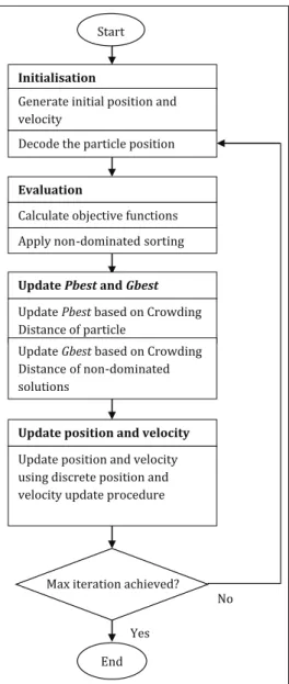
Figure 4 shows the working flow of MODPSO algorithm.
Initialisation
The number of particle (npar) and the maximum
num-ber of iteration (itermax) were set in this step. Then the
initial population known as swarm was produced by
generating thenparset of initial position (X) and
velo-city (V) that consists of permutation of integer from 1
to nin random orders. Next, the swarm was decoded
to generate feasible sequences according to the prece-dence constraint using topological sort procedure. Topological sort is an approach to establish feasible sequence by selecting only one available assembly task in each iteration. The topological sort procedure is pre-sented as follows:41
Procedure:Topological Sort Begin
n; number of tasks
st= 0; number of selected task
Whilest4n
s Establish available set
s st=st+ 1
s Select one task from available set and place in
stth position of feasible sequence
s Remove all outgoing arcs from selected task
s Eliminate selected task from precedence graph
End While End Procedure
In the procedure above, the available set consists of tasks without incoming arc. Then, one of the tasks in the available set was selected using a predetermined selection rule. There are a few selection rules regularly used such as random selection, weight-based selection and ordered-based selection. Next, all the outgoing arcs from selected task were removed and the selected task was eliminated from the graph to avoid selecting similar task. In this work, the selection rule for topological sort was set to follow the ordered-based selection. It means that the first available task found in the particle order will be selected to be placed in the feasible sequence.
Evaluation
In this step, the decoded feasible sequence was evalu-ated using the predefined objective functions. The objective functions were calculated using procedures and formulas in equations (1)–(3). Next, the non-dominated sorting was applied to establish the Pareto
set solution. This approach is adopted from Deb10 in
2002. The Pareto set was updated in every iteration by evaluating each particle with solution in the Pareto set.
Update
Pbest
and
Gbest
Pbestis the best personal particle solution whileGbest
is the best solution for all particles. To evaluate and
determine the Pbestand Gbest, a mechanism to select
the best solution within all particles is needed. For this
purpose,CD that provides the estimation of solutions
density surrounding that solution was used. ForPbest,
the CD was calculated within the solution in the
swarm, whereas theCDforGbestwas calculated within
the Pareto set. The following algorithm was used to
calculate theCDof each point in the setR.10
CDcalculation procedure:
Step 1: call the number of the solution inRas ڞ=|R|.
For eachiin the set, assigndi= 0.
Step 2: for each objective functionm= 1, 2,.,M, sort
the set in a descending order ofrm.
Step 3: for m= 1, 2,., M, assign maximum (maxm)
and minimum (minm) values for each objectivem.
Step 4: calculatedm
i for each objectivemfor solutioni
dmi = I m upiImlowi maxmminm ð4Þ
Step 5: calculate summation ofdm
i CDi= XM m= 1 dmi ð5Þ In equation (4), Im
upi is the nearest upper mth
objec-tive value for solutioni. Meanwhile,Im
lowi represents the
nearest lowermth objective value for solutioni. In this
case, if the objective value is located at the first or last
place in the rm, themaxmand minmvalues are used to
replace the nearest value, respectively.
ForPbest, if the current particle has largerCD
com-pared to the existing Pbest, the Pbestis replaced with
the current position; otherwise, the existing Pbest is
reused. Meanwhile, Gbest was selected as the highest
CD among all Pareto solutions. In the proposed
MODPSO,Gbestdoes not represent the most optimum
solution as in traditional PSO, but it will be the leader to update the swarm position and velocity for the next iteration.
Update position and velocity
The final step in MODPSO is to update swarm position and velocity. The purpose of this step is to establish
new swarm set that follows the current Pbest and
Gbest. In the original PSO, the position and velocity are updated using the following formulas
Xti+ 1=Xti+Vti+ 1 ð6Þ
Vti+ 1=c1Vit+c2(PbesttiX t
i) +c3(GbesttXti) ð7Þ
All the operations in equations (6) and (7) can be easily performed for the continuous problem. However, for the discrete problem, the following discrete position and velocity update procedure were proposed to replace the original operations.31,33
Subtraction operator (position2position). This operation
was found in equation (7), (Pbestt
iXti) and (Gbestt Xt
i) and produced the velocity. LetX1t= [x1,1,x1,2,x1,3,
x1,4,x1,5,x1,6,x1,7],X2t= [x2,1,x2,2,x2,3,x2,4,x2,5,x2,6,
x2,7] andV1t=X1t2X2t. In this case, ifx1andx2in the
jth position are equal, thenv1= 0. Otherwise,v1=x1.
Addition operator (position+velocity). For the addition of
position and velocity in equation (6), if thejth element
of velocity (vj) is equal to 0, thejth position value (xjt) is
inserted into thejth element of the new position (xjt+ 1).
In the meantime, ifvjis nonzero and does not appear in
the new position, then xjt+ 1=vj. Otherwise, xjt+ 1 is
equal to 0.
Multiplication operator (coefficient+velocity). This opera-tion was performed to make an adjustment on the
influence ofPbestandGbeston the new velocity. This
operation can be represented as V2=c3 V1, where
coefficient c2[0, 1] is used to control the effect of V1
that inherit inV2. For this purpose, a random number,
rand2[0, 1] is generated. If rand\c, v2=v1, or else,
v2= 0. In this work, coefficients c1,c2 andc3were set at 0.7.
Addition operator (velocity+velocity). This operation was performed to sum up the velocities in equation (7). For
new velocity,V=V1+V2, thejth element ofVcan be
derived as follows vj= v1,jifv1,j6¼0,v2,j= 0 v1,jifv1,j6¼0,v2,j6¼0,r\cp v2,j, otherwise 8 < : ð8Þ
In equation (8),ris a random number between 0 and 1,
while cp2[0, 1] is inheriting constant that influences
eitherv1orv2into new velocity.
Table 3 presents the comparison of the proposed MODPSO with NSGA-II, DPSO and MOPSO algo-rithms in terms of major algorithm stages. In general, the MODPSO algorithm applied similar strategies with NSGA-II for initialisation, evaluation and selection
stages, but different in regeneration stage. The
MODPSO regeneration strategy used discrete position and velocity update procedure that was adopted from
DPSO algorithm. Meanwhile, indifferent with
MOPSO, the proposed MODPSO used different selec-tion and regeneraselec-tion strategies to handle multi-objective problem.
Experimental design
In order to test the proposed MODPSO, the experi-mental design was set up. The main purpose of this experiment was to test the performance of the proposed MODPSO compared with other algorithms using a set of wide range of problem difficulties. In previous work, a tuneable test problem generator for ASP and ALB
has been developed.17The results indicate that the ASP and ALB problem difficulties can be increased using
larger number of tasks (n), lower order strength (OS),
lower time variability ratio (TV) and higher frequency
ratio (FR).
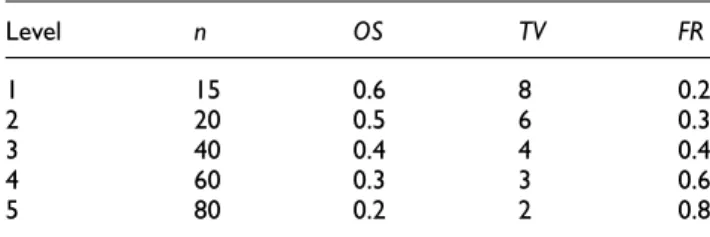
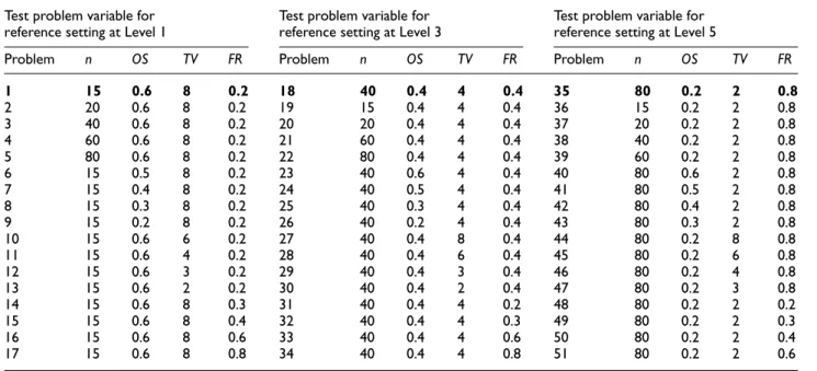
For experimental purpose, each of input variables was divided into five levels from low to high difficulty as in Table 4. Then a reference variable setting (datum) was selected as a baseline, while the rest of the problem variable setting was generated by changing only one variable value at a time. In total, there were 17 test problems (including reference setting) generated from one reference variable setting. In order to confirm algo-rithm performance, three different reference variable settings were used (Levels 1, 3 and 5). Therefore, the complete number of test problem that involved in this experiment was 51 problems as shown in Table 5, and the problem setting in bold (Problems 1, 18 and 35) represented the reference variable setting for Levels 1, 3 and 5, respectively.
The MODPSO for integrated ASP and ALB prob-lem was coded using MATLAB software. For the per-formance comparison purpose, six other algorithms used to optimise integrated ASP and ALB are as follows:
1. ACO: this algorithm has been used for simple ALB
problem in Bautista and Pereira.42 On the other
hand, the ACO algorithm has also been used in
integrated ASP and ALB.13 This algorithm was
selected based on its popularity.
2. Hybrid genetic algorithm (HGA): HGA has been
proposed by Chen et al.14 and selected based on
citation popularity for integrated ASP and ALB optimisation.
3. MOGA: this algorithm used in Choi et al.43 to
optimise ASP problem was chosen because GA is one of the most frequently used algorithms for
sol-ving and optimising ASP problems.1 In common
with this work, it used task-based representation for ASP problem.
4. NSGA-II: NSGA-II was introduced by Deb et al.35
in 2002. This algorithm was selected because of its popularity in multi-objective optimisation.
5. MOPSO: the MOPSO acronym was introduced by
Coello Coello and Lechuga29 to extend the PSO
application for Pareto-based multi-objective
T able 3. Comparison of the NSGA-II, DPSO , MOPSO and the pr oposed MODPSO . Algorithm stage NSGA-II DP SO MOPSO MODPSO Initialisation Random initial population Ran dom initial particles Random initial particles Random initial part icles Evaluation Individual fitness e valuation W eighted based e valuation Individual fitness e valuation Individual fitness e valuation Selection Best cr owding distance of non-dominated solution Best w eighted fitness Random selection fr om less density h yper cube of non-dominated solution Best cr owding distance of non-dominated solutio n Regeneration Cr ossov er and mutation operators Discr ete PSO pr ocedur e to update position and velocity Standar d PSO operators to update position and velocity Discr ete PSO pr ocedur e to update position and velocity NSGA-I I: non -dom inated sorting gen etic al gorithm II; DPSO: disc re te particle swarm optim isation; MOPS O: multi-objecti ve particle swa rm opti mis ation; MOD PSO: multi-objecti ve discr ete particle swarm optimisation .
Table 4. Level of tuneable input setting.
Level n OS TV FR 1 15 0.6 8 0.2 2 20 0.5 6 0.3 3 40 0.4 4 0.4 4 60 0.3 3 0.6 5 80 0.2 2 0.8
optimisation instead of weighted-based approach in earlier version.
6. DPSO: DPSO was proposed by Rameshkumar
et al.31for discrete problem. Instead of using
nor-mal mathematical operation to update position and velocity in PSO, this algorithm introduced spe-cial procedure to incorporate the discrete problem. The originality of all the above algorithms was retained, as proposed by the researchers. For example, the HGA and the MOGA that were previously encoded using permutation chromosome had been directly applied to the integrated ASP and ALB. Meanwhile, the ACO algorithm functioned by constructing the assembly sequence according to the pheromone level. Hence, different assembly sequences were generated by controlling the amount of pheromone level. Therefore, no modification was required to suit the algorithm to be integrated with ASP and ALB. Besides, the DPSO was also directly implemented because it was purposely proposed to address combinatorial problem.
On the other hand, the NSGA-II and the MOPSO were originally proposed to combat the continuous optimisation problem. In order to fit both algorithms to be integrated with ASP and ALB, the continuous value of chromosome/particle position had been defined as weight to determine the sequence of assembly
task. For instance, the particle positioned atX1= [0.35,
7.27, 2.41, 6.38, 2.12] was decoded into X1’ = [2 4 3
5 1], giving priority to the larger position value. With this approach, the originality of NSGA-II and MOPSO had been successfully preserved since the original chro-mosome/particle was directly evaluated.
In this work, the population or swarm size was set at 20 with 500 iterations. For each problem, 30 simulation
runs with different random seeds were performed and the output from each run was gathered and filtered to get the non-dominated solution.
Performance indicators
To evaluate the performance of each algorithm when dealing with different complexity problems, the
follow-ing performance indicators adopted from Deb10 and
Yoosefelahi et al.44were used:
1. Number of non-dominated solution in Pareto
opti-mal, h~: the number of non-dominated solution
generated by each algorithm in Pareto solution.
Higherh~shows better algorithm performance.
2. Error ratio (ER): the number of solution which is
not member of the Pareto optimal set divided by
the number of solution generated by algorithm q.
SmallerERshows better algorithm performance.
3. Generational distance (GD): GD finds an average
distance of solution with the nearest Pareto
opti-mal solution. Sopti-mallerGDprovides better algorithm
performance GDq= Psq i= 1 di sq ð9Þ
sqis the number of solution generated by algorithmq
di=minPk= 1 ffiffiffiffiffiffiffiffiffiffiffiffiffiffiffiffiffiffiffiffiffiffiffiffiffiffiffiffiffiffiffiffiffiffiffi XM m= 1 (f(mi)f(mk)) 2 v u u t ð10Þ
Table 5. Experimental design for integrated ASP and ALB. Test problem variable for
reference setting at Level 1
Test problem variable for reference setting at Level 3
Test problem variable for reference setting at Level 5
Problem n OS TV FR Problem n OS TV FR Problem n OS TV FR
1 15 0.6 8 0.2 18 40 0.4 4 0.4 35 80 0.2 2 0.8 2 20 0.6 8 0.2 19 15 0.4 4 0.4 36 15 0.2 2 0.8 3 40 0.6 8 0.2 20 20 0.4 4 0.4 37 20 0.2 2 0.8 4 60 0.6 8 0.2 21 60 0.4 4 0.4 38 40 0.2 2 0.8 5 80 0.6 8 0.2 22 80 0.4 4 0.4 39 60 0.2 2 0.8 6 15 0.5 8 0.2 23 40 0.6 4 0.4 40 80 0.6 2 0.8 7 15 0.4 8 0.2 24 40 0.5 4 0.4 41 80 0.5 2 0.8 8 15 0.3 8 0.2 25 40 0.3 4 0.4 42 80 0.4 2 0.8 9 15 0.2 8 0.2 26 40 0.2 4 0.4 43 80 0.3 2 0.8 10 15 0.6 6 0.2 27 40 0.4 8 0.4 44 80 0.2 8 0.8 11 15 0.6 4 0.2 28 40 0.4 6 0.4 45 80 0.2 6 0.8 12 15 0.6 3 0.2 29 40 0.4 3 0.4 46 80 0.2 4 0.8 13 15 0.6 2 0.2 30 40 0.4 2 0.4 47 80 0.2 3 0.8 14 15 0.6 8 0.3 31 40 0.4 4 0.2 48 80 0.2 2 0.2 15 15 0.6 8 0.4 32 40 0.4 4 0.3 49 80 0.2 2 0.3 16 15 0.6 8 0.6 33 40 0.4 4 0.6 50 80 0.2 2 0.4 17 15 0.6 8 0.8 34 40 0.4 4 0.8 51 80 0.2 2 0.6
wheref(i)
m is themth objective function value of solution
i and f(k)
m is the mth objective function value of kth
member of Pareto optimal.
4. Spacing: this indicator measures the relative distance between each solution
Spacing= ffiffiffiffiffiffiffiffiffiffiffiffiffiffiffiffiffiffiffiffiffiffiffiffiffiffiffiffiffiffi 1 N Xsq i= 1 (did) 2 v u u t ð11Þ
wherediis the distance between solutioniand the
near-est solution, whiledis the average of alldi. The smaller spacingindex shows better solution and has better space between each solution.
5. Maximum spread,Spreadmax: the spread of solution
found by each algorithm. Larger maximum spread is better Spreadmax= ffiffiffiffiffiffiffiffiffiffiffiffiffiffiffiffiffiffiffiffiffiffiffiffiffiffiffiffiffiffiffiffiffiffiffiffiffiffiffiffiffiffiffiffi XM i= 1 ( minfimaxfi)2 v u u t ð12Þ
Experimental results
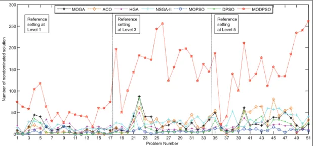
Figure 5 shows the number of the non-dominated
solu-tion in Pareto optimal (h~) for all test problems using
different algorithms. This figure shows that the pro-posed MODPSO performed better than other algo-rithms in all test problems. In the majority of test
problems, there was a significant gap between
MODPSO and other algorithms in terms ofh~ found.
According to the output pattern, larger problem size will come out with broader gaps between MODPSO and other algorithms.
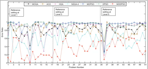
TheERfor all algorithms is presented in Figure 6.
From 51 test problems, MODPSO algorithms per-formed better in 82% of the problems. While the remaining 18% of problems was led by NSGA-II, where most of these problems involved larger task
numbers (60 and 80 tasks). However, the mean ofER
using MODPSO for all test problems remained the smallest (0.34) compared with NSGA-II (0.57) and other algorithms (between 0.81 and 0.93).
Meanwhile, Figure 7 presents theGDfor algorithms
throughout the test problems. For this indicator, MODPSO also performed better in 82% of the
prob-lems in almost similar probprob-lems as in ER. This is
because the GD was measured between the solutions
with the nearest Pareto solution. When the number of
the non-Pareto solution increased (higherER), the
aver-age of distance to Pareto solution would also increase. However, it still depends on how far the distance of non-Pareto with the Pareto solution. For example in
Problem 22, although theERusing MODPSO was
bet-ter than other algorithms, theGD using this algorithm
was in the third position after MOGA and ACO. It shows that the distance of non-Pareto solution in MODPSO was relatively larger than MOGA and ACO,
since these algorithms also produced goodh~for a
par-ticular problem.
Figure 8 shows the performance ofSpacingindicator
that leads to different algorithms. For this indicator, MOPSO algorithm performed better in 37% of test problems. Then it was followed with MODPSO (22%), HGA (18%), DPSO (15%), MOGA (6%) and ACO (2%).
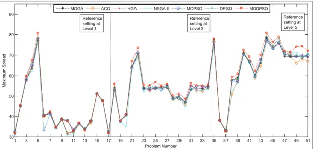
For maximum spread (Spreadmax) in Figure 9, all
algorithms show almost similar graph pattern with small gaps between one another. For this indicator, MODPSO algorithm performed better in 71% of test problems. In this case, MODPSO achieved better per-formance in the problem with the larger number of
Figure 6. Error ratio throughout test problems.
Figure 7. Generational distance throughout test problems.
tasks, as it performed better in all test problems with 60 and 80 tasks.
Figure 10 shows the average CPU time to complete 500 iterations for different algorithms. Based on the results, NSGA-II consistently required the highest
computational time compared with other algorithms. This is related to NSGA-II feature which combined the parent and offspring chromosomes in the evaluation stage. In other words, the number of evaluated chro-mosomes in NSGA-II was doubled compared with
Figure 9. Maximum spread throughout test problems.
other algorithms. On the other hand, MOPSO algorithm was the fastest due to the basic updating procedures implemented in this algorithm. The proposed MODPSO meanwhile was the second highest computational time behind the NSGA-II. Besides implementing the discrete
updating procedure, the proposed algorithm also
required additional time to adopt the non-dominated
sorting concept and calculateCDfor the leaders.
Discussion of results
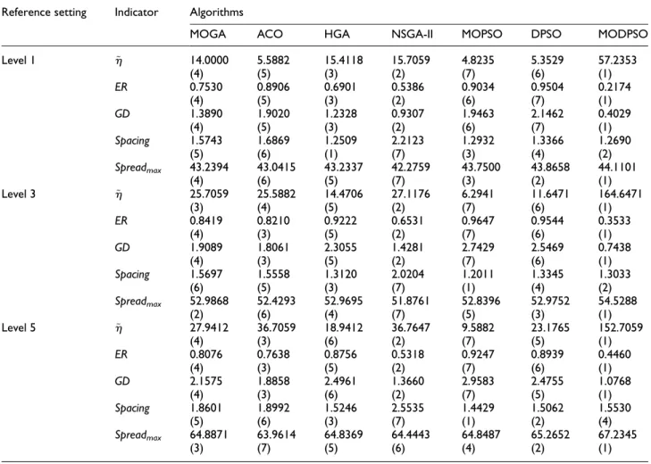
Table 6 presents the mean of performance indicators obtained using different reference variable settings. The number in bracket presents the algorithm ranking based on the mean of each indicator. According to this table, the MODPSO algorithm consistently performed
better inh~,ER, GDandSpreadmaxfor all the reference
settings. Meanwhile, for Spacing indicator, HGA
and MOPSO algorithms showed better performance than MODPSO. Based on this table, the proposed MODPSO algorithm came out with better performance
in all indicators except inSpacingindicator.
In Spacing indicator, all non-dominated solutions found by the particular algorithm were taken into
account, regardless of Pareto or non-Pareto solutions. This indicator showed the uniformity of the space between one solution and the nearest other. Thus, the algorithm that generated more non-dominated solu-tions has greater chances to produce better (smaller)
Spacing. However, the solution distribution is more
important in achieving better Spacing. This is because
the solutions that are only distributed to particular
side(s) of solution space will have better Spacing
com-pared with solutions that are distributed uniformly over the entire solution space, even though the number of non-dominated solution is much smaller. As an example in Problem 3, the numbers of non-dominated solution found using MODPSO and MOGA were 152 and 84,
respectively, but MOGA came out with betterSpacing
compared with MODPSO. Figure 11 shows the scatter-plot matrix for Problem 3 using both algorithms. From these figures, the MODPSO solution was distributed in larger solution space compared with MOGA.
Based on the means of the performance indicator, the algorithms with the basis of GA showed good per-formance behind the proposed MODPSO. The NSGA-II consistently showed impressive performance in three indicators behind MODPSO, although it did not
Table 6. Mean of performance indicators by the different reference settings. Reference setting Indicator Algorithms
MOGA ACO HGA NSGA-II MOPSO DPSO MODPSO
Level 1 h~ 14.0000 5.5882 15.4118 15.7059 4.8235 5.3529 57.2353 (4) (5) (3) (2) (7) (6) (1) ER 0.7530 0.8906 0.6901 0.5386 0.9034 0.9504 0.2174 (4) (5) (3) (2) (6) (7) (1) GD 1.3890 1.9020 1.2328 0.9307 1.9463 2.1462 0.4029 (4) (5) (3) (2) (6) (7) (1) Spacing 1.5743 1.6869 1.2509 2.2123 1.2932 1.3366 1.2690 (5) (6) (1) (7) (3) (4) (2) Spreadmax 43.2394 43.0415 43.2337 42.2759 43.7500 43.8658 44.1101 (4) (6) (5) (7) (3) (2) (1) Level 3 h~ 25.7059 25.5882 14.4706 27.1176 6.2941 11.6471 164.6471 (3) (4) (5) (2) (7) (6) (1) ER 0.8419 0.8210 0.9222 0.6531 0.9647 0.9544 0.3533 (4) (3) (5) (2) (7) (6) (1) GD 1.9089 1.8061 2.3055 1.4281 2.7429 2.5469 0.7438 (4) (3) (5) (2) (7) (6) (1) Spacing 1.5697 1.5558 1.3120 2.0204 1.2011 1.3345 1.3033 (6) (5) (3) (7) (1) (4) (2) Spreadmax 52.9868 52.4293 52.9695 51.8761 52.8396 52.9752 54.5288 (2) (6) (4) (7) (5) (3) (1) Level 5 h~ 27.9412 36.7059 18.9412 36.7647 9.5882 23.1765 152.7059 (4) (3) (6) (2) (7) (5) (1) ER 0.8076 0.7638 0.8756 0.5318 0.9247 0.8939 0.4460 (4) (3) (5) (2) (7) (6) (1) GD 2.1575 1.8858 2.4961 1.3660 2.9583 2.4755 1.0768 (4) (3) (6) (2) (7) (5) (1) Spacing 1.8601 1.8992 1.5246 2.5535 1.4429 1.5062 1.5530 (5) (6) (3) (7) (1) (2) (4) Spreadmax 64.8871 63.9614 64.8369 64.4443 64.8487 65.2652 67.2345 (3) (7) (5) (6) (4) (2) (1)
MOGA: multi-objective genetic algorithm; ACO: ant colony optimisation; HGA: hybrid genetic algorithm; NSGA-II: non-dominated sorting genetic algorithm II; MOPSO: multi-objective particle swarm optimisation; DPSO: discrete particle swarm optimisation; MODPSO: multi-objective discrete particle swarm optimisation;ER: error ratio;GD: generational distance.
perform well in Spacing and Spreadmax indicators.
Meanwhile, the MOGA algorithm showed medium performance in most of the indicators for all reference settings. By the calculated mean, this algorithm was located between the third and fourth ranks. However, HGA showed inconsistent performance from one refer-ence setting level to another. For the referrefer-ence setting at Level 1, HGA shows quite good performance at the third ranking. But when the reference setting was chan-ged to Levels 3 and 5, the HGA mean ranking dropped to the fourth and fifth positions, respectively.
On the other hand, the ACO algorithm showed improvement from one reference setting the level to
another forh~,ERandGD. On average, the ACO was
placed in the fifth rank among all algorithms. The remaining two algorithms, DPSO and MOPSO, were placed in the sixth and seventh ranks according to the indicator means. Both algorithms did not perform well
inh~, ERand GDbut showed quite impressive
perfor-mance inSpacingandSpreadmaxindicators.
The performance of DPSO showed that the algo-rithm designed with weighted objective functional approach was unsuitable for finding a non-dominated solution, although it used an efficient regeneration pro-cedure as in MODPSO. Meanwhile, the MOPSO’s per-formance showed that the original PSO operator to update position and velocity was not good enough for the discrete problem. On the other hand, the NSGA-II
that performed efficiently in three indicators showed
that the selection strategy based on CD of
non-dominated solution worked effectively, since the MODPSO that adopted similar strategy also did well. Based on the performance of NSGA-II and DPSO algorithms, the proposed MODPSO algorithm has inherited good features from NSGA-II and DPSO because the MODPSO algorithm mainly adopted stra-tegies from these algorithms.
The results in Table 6 also indicate that the proposed MODPSO consistently performed better than GA-based algorithms (i.e. MOGA, HGA and NSGA-II) for all the indicators exceptSpacingin all reference settings. It shows that the MODPSO was able to optimise inte-grated ASP and ALB problem from various difficulty levels efficiently compared with GA-based algorithms.
Statistical tests
To test the significance of the results, statistical tests were performed. In this case, analysis of variance (ANOVA) test was carried out to test whether there was any significant difference between the results obtained by an algorithm compared with other algo-rithms. The null hypothesis stated that there was no significant difference among all algorithm means. When the null hypothesis was accepted, it means that there was no significant improvement achieved by any
algorithms. The summary of ANOVA test is presented in Table 7.
In order to accept the null hypothesis, the
calcu-lated f-value must be smaller than the criticalf-value
(f*). Thef* obtained fromf-distribution table at 0.05
confidence interval was 3.86.45 Based on Table 7,
only the f-value for Spreadmax fulfilled the
require-ment to accept the null hypothesis. Meanwhile, thef
-values for h~,ER, GD andSpacingindicators showed
larger values compared with f*. It means that four of
the five performance indicators rejected the null hypoth-esis which brought the meaning that there were signifi-cant differences between algorithms. In this case, it shows that there were significant improvements achieved at least by one algorithm compared to others. Meanwhile, the
acceptance of null hypothesis by Spreadmax indicator
shows that all algorithms were able to explore the extreme minimum and maximum values in the search space.
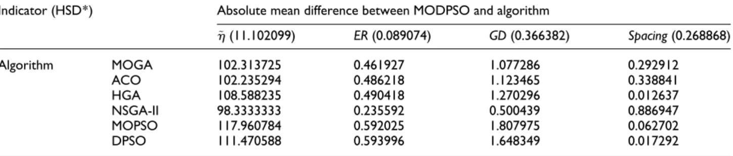
However, the ANOVA test did not tell us the exact algorithms that have significant mean differences. Therefore, a posteriori test known as the Tukey’s hon-estly significant different (HSD) test was performed to identify whether there was any significant improvement achieved by the proposed MODPSO compared to other algorithms. The Tukey’s HSD test was only con-ducted for the performance indicators that rejected the
null hypothesis (h~, ER, GD and Spacing) since only
these groups showed the significant difference between algorithms. The summary of the Tukey’s HSD test is presented in Table 8.
Table 8 presents the absolute mean difference between MODPSO and other algorithms. The number in bracket shows the critical HSD value (HSD*) that
was calculated based on the Tukey’s table.45When the
absolute mean difference between MODPSO and the particular algorithm is larger than HSD*, it means that the significant improvement has been identified between these two algorithms. Based on Table 8, the significant improvement was achieved by the proposed MODPSO
compared with all other algorithms for h~,ERandGD
indicators. In the meantime, the significant Spacing
improvements were observed between MODPSO and MOGA, ACO and NSGA-II, but not with HGA, MOPSO and DPSO. This result was consistent with earlier finding in Figure 8 and Table 6 that prioritised the HGA, MOPSO and DPSO algorithms together
with MODPSO forSpacingindicator.
The Tukey’s HSD test result explained that the pro-posed MODPSO performed well to converge to Pareto optimal solutions since the indicators that directly
linked with it (h~, ER and GD) showed significant
improvement compared with other algorithms. On the other hand, the MODPSO only showed significant improvement in some cases in terms of uniformity of the found solution. Meanwhile, no significant improve-ment was found for the solution spreading, although small difference as presented in Figure 9 was notified.
The proposed MODPSO algorithm showed better performance because of the fine-tuning feature towards the end of iterations. This feature is important in ASP and ALB, where small changes may lead to sudden
Table 8. Summary of Tukey’s HSD test.
Indicator (HSD*) Absolute mean difference between MODPSO and algorithm ~ h(11.102099) ER(0.089074) GD(0.366382) Spacing(0.268868) Algorithm MOGA 102.313725 0.461927 1.077286 0.292912 ACO 102.235294 0.486218 1.123465 0.338841 HGA 108.588235 0.490418 1.270296 0.012637 NSGA-II 98.3333333 0.235592 0.500439 0.886947 MOPSO 117.960784 0.592025 1.807975 0.062702 DPSO 111.470588 0.593996 1.648349 0.017292
HSD: honestly significant different; MODPSO: multi-objective discrete particle swarm optimisation;ER: error ratio;GD: generational distance; MOGA: multi-objective genetic algorithm; ACO: ant colony optimisation; HGA: hybrid genetic algorithm; NSGA-II: non-dominated sorting genetic algorithm II; MOPSO: multi-objective particle swarm optimisation; DPSO: discrete particle swarm optimisation.
Table 7. Summary of ANOVA test. ~
h ER GD Spacing Spreadmax
SSB 512147.60 14.30 121.93 35.03 183.90 SSW 301524.1 8.1442 137.805 74.207 72260.1 MSB 85358 2.38395 20.3224 5.83856 30.648 MSW 861.5 0.02327 0.3937 0.21202 206.457 f* 3.68 3.68 3.68 3.68 3.68 f 99.08 102.45 51.62 27.54 0.15
ER: error ratio;GD: generational distance; SSB: sum of square between groups; SSW: sum of square within groups; MSB: mean squares between groups; MSW: mean squares within groups;f*: critical f-value;f: calculated f-value.
improvement in the results. The discrete updating pro-cedure in MODPSO was designed to enable fine tuning towards the end of iterations. In PSO, all particles moved towards personal and global best solutions. According to the discrete updating procedure
(subtrac-tion operator (Xi2Xj)) in MODPSO, zero velocity was
given when similar elements inXi and Xj were found
(this is the case when all particles move towards the best solution at the end of iterations). When the major-ity of velocmajor-ity elements were 0, only small changes occurred in assembly sequence as presented by addition
operator (Xi+Vi). This feature allowed fine tuning of
the assembly sequences in MODPSO.
Conclusion
In this work, a MODPSO algorithm was proposed to optimise an integrated ASP and ALB problems. Indifferent with the existing algorithms, MODPSO that used Pareto-based approach to deal with multi-objective problem adopted discrete procedure instead of standard mathematical operators to update its posi-tion and velocity. A set of 51 test problems with differ-ent ranges of difficulties were used to test the performance of MODPSO compared with other algorithms.
The results show that the MODPSO performed bet-ter in all test problems in finding a non-dominated
solu-tion (h~), 82% inER, 82% inGD, 22% inSpacing and
71% inSpreadmax. Meanwhile, the result in Table 6
pre-sents that the MODPSO performed better in four of the five performance indicators in all difficulty levels. This result shows the proposed MODPSO successfully over-came the underperformance of GA-based algorithms for the test problem with a larger number of tasks.
A statistical test was conducted to identify any
signif-icant improvement achieved by the proposed
MODPSO. The statistical test concluded that the MODPSO showed significant improvement compared with other algorithms to converge to Pareto optimal solutions. In terms of solution uniformity, the signifi-cant improvement achieved by MODPSO was only applied to certain comparison algorithms. Furthermore, no significant improvement was achieved for the solu-tion spreading using the MODPSO. Therefore, it can be concluded that the proposed MODPSO has shown good performance in terms of solution quality towards Pareto optimal solutions.
Instead of specific application to optimise integrated ASP and ALB problem, the proposed MODPSO can also be used to optimise other types of discrete prob-lems represented using precedence graph. This includes the travelling salesman problem and vehicle routing problem with precedence constraint. However, the pro-posed MODPSO has limited performance in terms of
solution uniformity as attained by Spacing indicator.
Besides that, the CPU time for MODPSO is also among the highest within the comparison algorithms.
In future, an extensive effort to improve the solution uniformity and spreading is proposed to improve the quality of the overall solution. This might be achieved by hybridising the MODPSO with different algorithms with better solution spread. Besides, the MODPSO algorithm could be tested with higher complexity assembly problems, such as mixed model, as well as two-sided and parallel lines, in order to better under-stand the behaviour of the algorithm at varied com-plexity levels. Furthermore, the application of the algorithm to the industrial problem is also suggested.
Declaration of conflicting interests
The author(s) declared no potential conflicts of interest with respect to the research, authorship and/or publica-tion of this article.
Funding
The author(s) disclosed receipt of the following finan-cial support for the research, authorship, and/or publi-cation of this article: The author(s) received financial support from Universiti Malaysia Pahang and Ministry of Higher Education, Malaysia for the research and publication of this article.
References
1. Rashid MFF, Hutabarat W and Tiwari A. A review on assembly sequence planning and assembly line balancing optimisation using soft computing approaches.Int J Adv Manuf Tech2011; 59(1–4): 335–349.
2. Hamta N, Shirazi MA and Ghomi SF. A bi-level pro-gramming model for supply chain network optimiza-tion with assembly line balancing and push-pull strategy. Proc IMechE, Part B: J Eng Manuf 2016; 230(6): 1127–1143.
3. Li M, Zhang Y, Zeng B, et al. The modified firefly algo-rithm considering fireflies’ visual range and its applica-tion in assembly sequences planning. Int J Adv Manuf Tech2015; 82(5–8): 1381–1403.
4. Marian RM. Optimisation of assembly sequences using genetic algorithm. PhD Thesis, University of South Aus-tralia, Adelaide, SA, AusAus-tralia, 2003.
5. Tseng H-E and Tang C-E. A sequential consideration for assembly sequence planning and assembly line balancing using the connector concept.Int J Prod Res2006; 44(1): 97–116.
6. Ghandi SS and Masehian E. A breakout local search (BLS) method for solving the assembly sequence plan-ning problem.Eng Appl Artif Intel2015; 39: 245–266. 7. Becker C and Scholl A. A survey on problems and
meth-ods in generalized assembly line balancing. Eur J Oper Res2006; 168(3): 694–715.
8. Sungur B and Yavuz Y. Assembly line balancing with hierarchical worker assignment. J Manuf Syst2015; 37: 290–298.
9. Haddadzade M, Razfar MR and Zarandi MHF. Multi-part setup planning through integration of process plan-ning and scheduling.Proc IMechE, Part B: J Eng Manuf
10. Deb K. Multi-objective optimization using evolutionary algorithms. Chichester: John Wiley & Sons, 2002. 11. Luke S.Essentials of metaheuristics. 1st ed. Palm Springs,
CA: Lulu, 2010.
12. Yang Z, Lu C and Zhao HW. An ant colony algorithm for integrating assembly sequence planning and assembly line balancing. Appl Mech Mater 2013; 397–400: 2570–2573.
13. Lu C and Yang Z. Integrated assembly sequence planning and assembly line balancing with ant colony optimization approach.Int J Adv Manuf Tech2016; 83(1): 243–256. 14. Chen R, Lu K and Yu S. A hybrid genetic algorithm
approach on multi-objective of assembly planning prob-lem.Eng Appl Artif Intel2002; 15: 447–457.
15. Tseng H-E, Chen M-H, Chang C-C, et al. Hybrid evolu-tionary multi-objective algorithms for integrating assem-bly sequence planning and assemassem-bly line balancing.Int J Prod Res2008; 46(21): 5951–5977.
16. Wang HS, Che ZH and Chiang CJ. A hybrid genetic algorithm for multi-objective product plan selection prob-lem with ASP and ALB.Expert Syst Appl 2012; 39(5): 5440–5450.
17. Ab Rashid MFF, Hutabarat W and Tiwari A. Develop-ment of a tunable test problem generator for assembly sequence planning and assembly line balancing. Proc IMechE, Part B: J Eng Manuf2012; 226(11): 1900–1913. 18. Xinchao Z. A perturbed particle swarm algorithm for
numerical optimization. Appl Soft Comput 2010; 10(1): 119–124.
19. Kennedy J and Eberhart R. Particle swarm optimization. In:Proceedings of IEEE international conference on neural networks, Perth, Australia, 27 November-1 December 1995, pp.1942–1948. New York: IEEE.
20. Shuang B, Chen J and Li Z. Microrobot based micro-assembly sequence planning with hybrid ant colony algo-rithm.Int J Adv Manuf Tech2007; 38(11–12): 1227–1235. 21. Gao J, Sun L, Wang L, et al. An efficient approach for type II robotic assembly line balancing problems.Comput Ind Eng2009; 56(3): 1065–1080.
22. Elbeltagi E, Hegazy T and Grierson D. Comparison among five evolutionary-based optimization algorithms.
Adv Eng Inform2005; 19(1): 43–53.
23. Mukund Nilakantan J and Ponnambalam SG. Robotic U-shaped assembly line balancing using particle swarm optimization.Eng Optimiz2015; 48(2): 231–252.
24. Liu CY and Wen HJ. Application of multi-objective cul-ture particle swarm optimization in complex product assembly line balancing.Adv Mater Res 2013; 694–697: 3526–3530.
25. Li M, Wu B, Hu Y, et al. A hybrid assembly sequence planning approach based on discrete particle swarm opti-mization and evolutionary direction operation.Int J Adv Manuf Tech2013; 68(1–4): 617–630.
26. Hamta N, Fatemi Ghomi SMT, Jolai F, et al. A hybrid PSO algorithm for a multi-objective assembly line balan-cing problem with flexible operation times, sequence-dependent setup times and learning effect. Int J Prod Econ2013; 141(1): 99–111.
27. Xing Y and Wang Y. Assembly sequence planning based on a hybrid particle swarm optimisation and genetic algo-rithm.Int J Prod Res2012; 50: 7303–7312.
28. Nearchou AC. Maximizing production rate and work-load smoothing in assembly lines using particle swarm optimization.Int J Prod Econ2011; 129(2): 242–250.
29. Coello Coello CA and Lechuga MS. MOPSO: a proposal for multiple objective particle swarm optimization. In:
Proceedings of the 2002 congress on evolutionary computa-tion, Honolulu, HI, 12–17 May 2002, pp.1051–1056. Washington, DC: IEEE Computer Society.
30. Tseng Y-J, Chen J-Y and Huang F-Y. A particle swarm optimisation algorithm for multi-plant assembly sequence planning with integrated assembly sequence planning and plant assignment.Int J Prod Res2010; 48(10): 2765–2791. 31. Rameshkumar K, Suresh RK and Mohanasundaram KM. Discrete particle swarm optimization (DPSO) algo-rithm for permutation flowshop scheduling to minimize makespan.Adv Nat Computation2005; 3612: 572–581. 32. Jianping D, Chun S and Jun L. A discrete particle swarm
optimization algorithm for assembly line balancing problem of type 1. In:Proceedings of the 2011 third inter-national conference on measuring technology and mecha-tronics automation, Shanghai, China., 6–7 January 2011, pp. 44–47. Washington DC: IEEE Computer Society. 33. Lv H and Lu C. An assembly sequence planning
approach with a discrete particle swarm optimization algorithm.Int J Adv Manuf Tech2010; 50(5–8): 761–770. 34. Wang Y and Liu JH. Chaotic particle swarm
optimiza-tion for assembly sequence planning. Robot Cim: Int Manuf2010; 26(2): 212–222.
35. Deb K, Member A, Pratap A, et al. A fast and elitist mul-tiobjective genetic algorithm. IEEE Trans Evol Comput
2002; 6(2): 182–197.
36. Rashid MFF, Tiwari A and Hutabarat W. An integrated representation scheme for assembly sequence planning and assembly line balancing. In: Proceedings of the 9th international conference on manufacturing research, Glas-gow, 6–8 September 2011, pp.125–131. Glasgow Caledo-nian University.
37. Qu S and Jiang Z. A memetic algorithm approach for batch-model assembly line balancing problem of sub-block in shipbuilding.Proc IMechE, Part B: J Eng Manuf
2014; 228(10): 1290–1304.
38. Whitney DE.Mechanical assemblies: their design, manu-facture, and role in product development(vol. 1). Oxford: Oxford University Press, 2004.
39. Yu H, Yu JP and Zhang WL. An particle swarm optimi-zation approach for assembly sequence planning. Appl Mech Mater2009; 16–19: 1228–1232.
40. Lv HG, Lu C and Zha J. A hybrid DPSO-SA approach to assembly sequence planning. In: 2010 IEEE interna-tional conference on mechatronics and automation, Xi’an, China, 4–7 August 2010, pp.1998–2003. New York: IEEE.
41. Moon C, Kim J, Choi G, et al. An efficient genetic algo-rithm for the traveling salesman problem with precedence constraints.Eur J Oper Res2002; 140(3): 606–617. 42. Bautista J and Pereira J. Ant algorithms for a time and
space constrained assembly line balancing problem.Eur J Oper Res2007; 177(3): 2016–2032.
43. Choi YK, Lee DM and Bin Cho Y. An approach to -multi-criteria assembly sequence planning using genetic algorithms.Int J Adv Manuf Tech2008; 42(1–2): 180–188. 44. Yoosefelahi A, Aminnayeri M, Mosadegh H, et al. Type II robotic assembly line balancing problem: an evolution strategies algorithm for a multi-objective model.J Manuf Syst2012; 31(2): 139–151.
45. Coolidge FL. Statistics: a gentle introduction. London: SAGE, 2000.