Fixed-time Stabilization of Second-order Systems
with Unknown Nonlinear Inherent Dynamics
Yang Liu
The Seventh Research Division School of Automation Science
and Electrical Engineering Beihang University (BUAA)
Beijing, China [email protected]
Hong Yue
Department of Electronic and Electrical Engineering
University of Strathclyde Glasgow, U.K. [email protected]
Wei Wang
School of Automation Science and Electrical Engineering Beihang University (BUAA)
Beijing, China [email protected]
Abstract—This paper studies the fixed-time stabilization con-trol for a class of second-order systems with unknown nonlinear dynamics and external disturbance. To achieve the fixed-time stability, two polynomial feedbacks, one with fractional exponent and the other with exponent greater than 1, are exploited in the sliding surface design. Then, considering the unknown nonlinear dynamics and the external disturbance, the unit-vector technique, coupled with the upper bounds related to the Lipschitz condition of nonlinear dynamics and the uncertain disturbance, is utilized to the fixed-time stability controller based on the designed sliding surface function. Finally, a forced pendulum system is used as case study example to examine the effectiveness of the developed design framework.
Index Terms—fixed-time stability, sliding surface, nonlinear dynamics, external disturbance
I. INTRODUCTION
The finite-time stability and control of dynamic systems have been intensively investigated in recent studies, in which the stability is realized over a finite time interval, and the finite time is called the settling time or the convergence time. The finite-time stability is regarded as of more advantages than the classic Lyapunov asymptotic stability in many real applications, such as robot and vehicle systems [1]- [2] and spacecrafts [3]- [4]. One key issue in finite-time stability and control is the estimation of the settling time, which is a function depending on the initial conditions of system. This would lead to inconvenience in applications since the initial conditions of many practical systems are hard to be accurately obtained or even impossible to be known in advance. To solve this problem, the fixed-time stability control method was further developed by Polyakov [10], and then attracted the attention of many researchers. In this line of studies, it is required that the system is globally finite-time stable and the settling-time is bounded by a fixed constant independent of the initial conditions.
Compared with the extensive study on finite-time stability [5]- [9], there are fewer results for the fixed-time stability research. In [10], Polyakov derived a sufficient condition to
This work was supported by the NSFC (61473015, 61327807, 61520106010, 61503231), and the Fundamental Research Funds for the Central Universities.
ensure the fixed-time stability of uncertain linear plants and an estimation of the settling time was also given. For a linear sin-gle input system, an implicit Lyapunov function method was applied to establish certain criteria for the fixed-time stability in [11]. In [12], a general approach was provided to reveal the essence of finite-time stability and fixed-time convergence for the considered system, and conditions for finite-time and fixed-time convergence were derived. For a SISO dynamic system, it was shown that any finite-time convergent homogeneous sliding mode controller could be transformed into a fixed-time convergent one, featuring an upper bound of convergence time [13]. All the above research aims at linear dynamic systems, however, nonlinear systems are widely prevalent in applica-tions. For a class of first-order nonlinear systems, the fixed-time stability and the fixed-fixed-time synchronization of coupled discontinuous neural networks were investigated under the framework of Filippov solution [14]. Recently, Zuo et al. [15] considered the fixed-time stability of a class of second-order multi-variable nonlinear systems with matched uncertainties, and proposed a multi-variable sliding mode controller based on a set of nonlinear coupled sliding surfaces. Note that nonlinear functions of the controlled dynamics are used in the controller design, which implies that the nonlinear dynamics has to be known in advance. Nevertheless, the nonlinear dynamics of the controlled plant is generally more difficult to establish or even cannot be obtained.
Lyapunov tools. Meanwhile, the upper bound of the settling time is given, which only depends on the parameters in the designed stable controller, regardless of the initial conditions. To avoid the control singularity in practical implementations, a singularity-induced term, which results from the differentiation of the term with fractional exponent, is substituted by a saturation function of a given threshold. Finally, the proposed fixed-time stability controller is applied to a forced pendulum system.
The rest of this paper is organized as follows. In Section II, basic concepts and a preliminary result on fixed-time stability are briefly recalled, based on which the problem statement is made. In Section III, the fixed-time stability problem is addressed for a second-order system with unknown nonlinear dynamics, while the system with uncertain external disturbances is further considered in Section IV. A forced pendulum example is studied in Section V to illustrate the effectiveness of proposed control design methods. Finally, the conclusion is drawn in Section VI.
II. PRELIMINARIES ANDPROBLEMSTATEMENT A. Preliminaries
Consider the system
˙
x(t)∈F(t,x(t)),x(0) =x0, (1) where x(t) ∈Rm is the state, F : R+×Rm →Rm is an upper semi-continuous convex-valued mapping, such that the set F(t,x(t)) is non-empty for any (t,x(t))∈R+×Rm and
F(t,0) =0 fort>0.
Definition 1: [16] The origin of system (1) is a globally finite-time equilibrium if there is a function T :Rm→R+ such that for all x0∈Rm, the solutionx(t,x0)of system (1) is defined and limt→T(x0)x(t,x0) =0.T(x0)is called the settling time function.
Definition 2: [10] The origin of system (1) is a globally fixed-time equilibrium if it is globally finite-time stable and the settling time function T(x0)is bounded by some positive numberTmax>0, i.e., T(x0)≤Tmax,∀x0∈Rm.
Denote D∗ϕ(t) as the upper Dini derivative of a function
ϕ(t), which is defined as D∗ϕ(t):=lim
h→0+sup(ϕ(t+h)− ϕ(t))/h. The following conclusion can be drawn for the fixed-time stability analysis in this paper.
Lemma 1: [17] If there exists a continuous radially un-bounded functionV :Rm→R+∪ {0}such that
1)V(0) =0⇒x=0, and
2) any solution of (1) satisfies the inequality
D∗V(x(t))≤ −αVp(x(t))−βVq(x(t)) (2)
for some α,β > 0 and p >1 >q >0, then the origin of the system is globally fixed-time stable and the settling time function T(x0) is uniformly bounded by a computable constant, i.e.,
T(x0)≤Tmax:=α(p1−1)+β(11−q). (3)
Remark 1:Compared with (3), a less conservative estimate for the upper bound of settling time function T(x0) can be derived as
T(x0)≤ µπ
2pαβ (4)
if p=1+µ1 andq=1−µ1 are satisfied with µ>1, as given in the reference [17].
B. Problem Statement
Consider the following second-order multi-variable system ½
˙
x1(t) =x2(t) ˙
x2(t) =f(x) +u(t) (5)
with the initial condition x(0) = x0, where x(t) = [xT
1(t)xT2(t)]T ∈R2n denotes the state vector, t ∈[0,∞) is the time variable, f(x):R2n→Rn is the unknown nonlinear dynamics, and u(t)∈Rn is the control input. The control objective is to design a controller for the nonlinear system (5) such that the origin of the closed-loop system is a globally fixed-time equilibrium. The time variable t is omitted in the following controller design and stability analysis for a concise expression. As to the unknown nonlinear dynamics, the following assumption is made.
Assumption 1:The continuous nonlinear function f(x) sat-isfies the following Lipschitz condition
kf(ξ)−f(η)k ≤βkξ−ηk (6)
for ∀ξ,η∈Rn and ∀t≥0, where β is a positive constant scalar.
Remark 2:According to Assumption 1, we have
kf(x)−f(0)k ≤βkxk,∀x∈R2n, (7)
from which it is derived that
|kf(x)k −γ| ≤ kf(x)−f(0)k ≤βkxk (8)
withkf(0)k:=γ. From (8), it follows that
kf(x)k −γ≤βkxk, (9)
and then the inequality
kf(x)k ≤γ+βkxk (10)
is finally obtained by Assumption 1.
III. FIXED-TIMESTABILITY OFSECOND-ORDER NONLINEARSYSTEMS
To realize the fixed-time stability of nonlinear system (5), we firstly propose the following sliding surface:
whereα2,β2>0, p2>1, 1/2<q2<1. Then the control input is designed as
u=−α2[I+ (p2−1)x1x
T
1 kx1k]kx1k
p2−1x 2
−β2[I+ (q2−1)x1x
T
1 kx1k]kx1k
q2−1x
2−α1kskp1−1s
−β1kskq1−1s−η1kxkksks−η2ksks ,
(12)
whereα1,β1>0, η1≥β,η2≥γ, p1>1 and 0<q1<1. To proceed, we present a useful lemma, based on which we can obtain the main result as stated in Theorem 1 later on.
Lemma 2: [15] Consider a first-order multi-variable system
˙
x=−αkxkp−1x−βkxkq−1x, (13)
wherex∈Rn,α,β>0,p>1 and 0<q<1. Then, the system is globally fixed-time stable at the origin and the settling time estimate is given by (3).
Remark 3: Rewrite the sliding surface (11) as
s=x2+α2 x1
kx1kkx1k
p2+β 2 x1
kx1kkx1k
q2 (14)
with p2>1, 1/2<q2<1. Note that in (14), there are two polynomial feedbacks with fractional exponent and exponent greater than 1, respectively. In fact, after achieving the ideal sliding motion withs=0, the first polynomial term dominates the convergence speed for kx1k À1, while if kx1k ¿1, the second polynomial term is the dominant one.
Theorem 1: For the second-order multi-variable system (5) with unknown nonlinear dynamics satisfying Assumption 1, the global fixed-time stability is realized at the origin under the proposed controller (12), and the upper bound of the settling time is given by
T(x0)≤ 2
∑
i=1 [ 1
αi(pi−1)+ 1
βi(1−qi)]. (15)
Proof: The time derivative of s along the trajectory of
system (5) is calculated by
˙
s=f(x) +u+α2[I+ (p2−1)x1x
T
1 kx1k]kx1k
p2−1x 2
+β2[I+ (q2−1)x1x
T
1 kx1k]kx1k
q2−1x 2.
(16)
Substituting the controller (12) into (16) yields
˙
s=f(x)−α1kskp1−1s−β1kskq1−1s−η1kskkxks−η2ksks . (17)
Define the Lyapunov function V(s) =sTs/2, it can be derived that
D∗V(s)
≤ −α1kskp1+1−β1kskq1+1+kskkf(x)k −η1kxkksk −η2ksk ≤ −α1kskp1+1−β1kskq1+1+ksk(γ+βkxk)−η1kxkksk
−η2ksk
=−α1kskp1+1−β1kskq1+1−(η1−β)kxkksk −(η2−γ)ksk ≤ −α1kskp1+1−β1kskq1+1
=−α1(2V) p1+1
2 −β1(2V) q1+1
2 .
(18)
Let y=√2V and ˙y=V˙/√2V, from which and (18) it is obtained that
˙
y≤ −α1yp1−β1yq1. (19) According to Lemma 1, we have that the terms(t)approaches zero with a finite settling time bounded by
T1:=α 1 1(p1−1)+
1
β1(1−q1). (20) Till now, it has been proved thats(t) =0 for allt≥T1. Then combining with (11), we find that the corresponding reduced-order motion is governed by
˙
x1=−α2x1kx1kp2−1−β2x1kx1kq2−1. (21) According to Lemma 2, the fixed-time stability of (21) is achieved at the origin and the upper bound of settling time is given by
T2:=α 1 2(p2−1)+
1
β2(1−q2). (22) Thus, x1(t) =0 for ∀t≥T1+T2, from which it also follows that x2(t) =x˙1(t) =0 for∀t≥T1+T2.
To summarize, the nonlinear system (5) with the control input (12) is globally fixed-time stable at the origin with the settling time bounded byT(x0)≤T1+T2, whereT1andT2are positive constants independent of the initial conditions. This
completes the proof. ¤
Remark 4: It should be noted that the control input is not well defined in the set {(x1,x2)|x1=0,x26=0}, where the singularity results from the term kx1kq2−1x2 in (12) with q2<1. Furthermore, we can obtain the following controller associated with the ideal sliding motion by substitutingx2= −α2x1kx1kp2−1−β2x1kx1kq2−1into (12), that is,
u=α2[I+ (p2−1)x1x
T
1 kx1k]
×(α2kx1k2p2−1+β2kx1kp2+q2−1) x1 kx1k
+β2[I+ (q2−1)x1x
T
1 kx1k]
×(α2kx1kp2+q2−1+β2kx1k2q2−1) x1 kx1k
Then by observing the obtained expression in (23), it can be seen that the control input is always well defined during the sliding motion if 1/2<q2<1. Therefore, the singularity of controller can be avoided for s=0 by imposing the requirement 1/2<q2<1 to the designed controller (12).
To avoid the singularity occurrence of the proposed fixed-time stability controller during the whole motion process, we introduce the following saturation function
satε(z) =sign(z)·min{|z|,ε} (24) into (12), where z∈R andε is a threshold parameter. To be specific, applying (24) to (12) results in the following amended controller
u=−α2[I+ (p2−1)x1x
T
1 kx1k]kx1k
p2−1x2
−β2[I+ (q2−1)x1x
T
1 kx1k]kx1k
q2sat ε(kxx2
1k)−α1ksk
p1−1s
−β1kskq1−1s−η 1kxk
ksks−η2
s ksk,
(25)
where the saturation function satε(·) is used componentwise, i.e.,
satε(kxx2
1k) = [satε( x21
kx1k)· · ·satε( x2n
kx1k)]
T
withx2= [x21x22· · ·x2n]T.
Theorem 2: For the second-order multi-variable system (5) with unknown nonlinear dynamics satisfying Assumption 1, the global fixed-time stability is realized at the origin under the nonsingular controller (25), and the upper bound of the settling time is given by
T(x0)≤ 2
∑
i=1 [ 1
αi(pi−1)+ 1
βi(1−qi)] +Tε1, (26) whereTε1is a small time margin to account for the influence of the saturation manipulation to the convergence time.
Proof: The above result can be easily obtained by
combin-ing Theorem 1 with the analysis method to deal with saturation functions in Theorem 2 of [15]. Hence, the specific proof is
omitted here. ¤
IV. FIXED-TIMESTABILITY OFDISTURBEDSYSTEMS Consider the nonlinear second-order system with external disturbances:
½ ˙
x1(t) =x2(t) ˙
x2(t) =f(x) +u(t) +d(t), (27)
whered(t)∈Rn is the unknown external disturbance.
Assumption 2:There exists a known positive functionσ(t):
R+→Rsuch that
kd(t)k ≤σ(t) (28)
for ∀t≥0.
For the fixed-time stability problem of system (27), the following controller is developed
u=−α2[I+ (p2−1)x1x
T
1 kx1k]kx1k
p2−1x2
−β2[I+ (q2−1)x1x
T
1 kx1k]kx1k
q2−1x
2−α1kskp1−1s
−β1kskq1−1s−η 1kxk
ksks−(η2+θ) s ksk
(29)
with a positive function θ satisfying θ≥σ.
Theorem 3: For the disturbed nonlinear system (27) satis-fying Assumptions 1 and 2, the global fixed-time stability is realized at the origin under the proposed controller (29), and the upper bound of the settling time is provided by (15).
Proof: The time derivative of sliding surface s along the
trajectory of system (27) is
˙
s=f(x) +u+d+α2[I+ (p2−1)x1x
T
1 kx1k]kx1k
p2−1x 2
+β2[I+ (q2−1)x1x
T
1 kx1k]kx1k
q2−1x 2.
(30)
Applying the controller (29) into (30) leads to
˙
s=f(x) +d−α1kskp1−1s−β1kskq1−1s−η1kxk
ksks
−(η2+θ) s ksk.
(31)
Then the upper Dini derivative of the Lyapunov function V(s) =sTs/2 satisfies the following
D∗V(s)
≤ −α1kskp1+1−β1kskq1+1+kskkf(x)k+kskkdk −η1kxkksk −(η2+θ)ksk
≤ −α1kskp1+1−β1kskq1+1+ksk(γ+βkxk) +kskσ−η1kxkksk −(η2+θ)ksk =−α1kskp1+1−β1kskq1+1−(η
1−β)kxkksk −(η2−γ)ksk −(θ−σ)ksk
≤ −α1kskp1+1−β1kskq1+1
=−α1(2V) p1+1
2 −β1(2V) q1+1
2 .
(32)
By Lemma 2,s(t) approaches zero with a finite settling time bounded by (20). To proceed, substitution of s=0 into (11) results in (21), which will realize the fixed-time stability at the origin with the settling time bounded by (22). Combining the above two motion processes, we can conclude that the disturbed nonlinear system (27) with controller (29) is globally fixed-time stable at the origin with the settling time
upper-bounded byT(x0)≤T1+T2. ¤
Applying the saturation function (24) into (29), the nonsin-gular control input is derived as follows:
u=−α2[I+ (p2−1)x1x
T
1
kx1k]kx1k
p2−1x2
−β2[I+ (q2−1)x1x
T
1 kx1k]kx1k
q2sat ε( x2
kx1k)−α1ksk
p1−1s
−β1kskq1−1s−η1kxk
ksks−(η2+θ) s ksk,
(33)
and the following stability result can be obtained by the proofs of the established Theorem 3 and Theorem 2 in [15].
Theorem 4: For the second-order system (27) satisfying Assumptions 1 and 2, the global fixed-time stability is realized at the origin under the nonsingular controller (33), and the upper bound of the settling time is provided by
T(x0)≤ 2
∑
i=1 [ 1
αi(pi−1)+ 1
βi(1−qi)] +Tε2, (34) whereTε2is a small time margin to account for the saturation manipulation.
Remark 6:Similar to Remark 1, ifpi=1+1/µiandqi=1− 1/µi withµi>1 fori=1,2, then less conservative estimates for the upper bound of settling time in Theorems 2 and 4 can be respectively calculated as
T(x0)≤ 2
∑
i=1 πµi 2pαiβi
+Tε1, (35) and
T(x0)≤ 2
∑
i=1 πµi 2pαiβi
+Tε2. (36) V. SIMULATION
Consider a forced pendulum system with the following nonlinear dynamics
½ ˙ x=v
˙
v=−sin(x)−0.25v+1.5cos(2.5t)+u+ω, (37)
where x,v∈R represent the position and the velocity of pendulum, respectively.
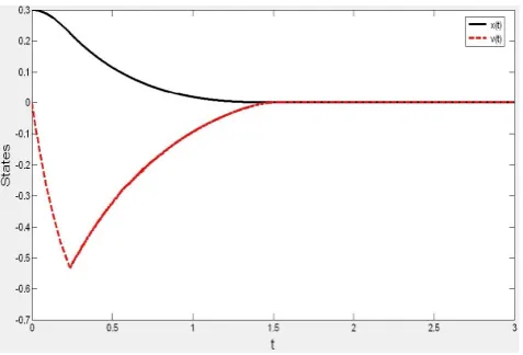
Firstly, for the system (37) without disturbances, the con-troller (25) is applied with parameters αi =βi =1, pi = 1+1/µi and qi=1−1/µi for i=1,2, where µ1=1.5 and µ2=2.5. By (35), the estimated upper bound of the settling time is larger than 6.2832 seconds. The closed-loop responses are shown in Fig. 1, from which it can be seen that the position and the velocity of pendulum converge to zeros within 2 seconds.
[image:5.595.319.558.48.210.2]Subsequently, for the system (37) with the external distur-bance d=1.5cos(v), the controller (33) is used with θ=2. In this case, the robust performance of closed-loop system is given in Fig. 2, in which the desired fixed-time stability is also realized.
[image:5.595.317.557.239.402.2]Fig. 1. State trajectories of the forced pendulum.
Fig. 2. State trajectories of the forced pendulum with external disturbances.
VI. CONCLUSIONS
This paper solves the fixed-time stabilization problem for a class of second-order multi-input systems with unknown nonlinear dynamics and external disturbances. To be specific, fixed-time stabilization control frameworks are respectively proposed for the nonlinear controlled objective and the dis-turbed uncertain system. It is explicitly demonstrated that the closed-loop system will realize stability within a fixed time related to the parameters of the proposed controller. The effectiveness of the developed control design method is verified by its applications to a forced pendulum system.
REFERENCES
[1] W. Huang, Y.N. Yang, and C.C. Hua, Fixed-time tracking control ap-proach design for nonholonomic mobile robot.Proceedings of the 35th Chinese Control Conference, 2016, 1934-1768.
[2] Y.M. Jia, Robust control with decoupling performance for steering and traction of 4WS vehicles under velocity-varying motion.IEEE Transac-tions on Control Systems Technology, 8(3): 554-569, 2000.
[3] H. Du, S. Li, and C. Qian, Finite-time attitude tracking control of spacecraft with application to attitude synchronization.IEEE Transactions on Automatic Control, 56, 2711C2717, 2011.
[5] E. Moulay and W. Perruquetti, Finite time stability conditions for nonau-tonomous continuous systems.International Journal of Control, 81, 797-803, 2008.
[6] S.P. Bhat and D.S. Bernstein, Finite-time stability of continuous au-tonomous systems.SIAM Journal on Control and Optimization, 38, 751-766, 2000.
[7] S.G. Nersesov, W.M. Haddad, and Q. Hui, Finite time stabilization of nonlinear dynamical systems via control vector Lyapunov functions.
Journal of the Franklin Institute, 345, 819-837, 2008.
[8] A. Zavala-Rio,and I. Fantoni,. Global finite-time stability characterized through a local notion of homogeneity.IEEE Transactions on Automatic Control, 59, 471-477, 2014.
[9] H. Yang, B. Jiang, and J. Zhao, On finite-time stability of cyclic switched nonlinear systems.IEEE Transactions on Automatic Control, 60, 2201-2206, 2015.
[10] A. Polyakov, Nonlinear feedback design for fixed-time stabilization of linear control systems. IEEE Transactions on Automatic Control, 57, 2106-2110, 2012.
[11] A. Polyakov, D. Efimov, and W. Perruquetti, Finite-time and fixed-time stabilization: implicit Lyapunov function approach.Automatica, 51, 332-340, 2015.
[12] W. Lu, X. Liu, and T. Chen, A note on finite-time and fixed-time stability.Neural Networks, 81, 11-15, 2016.
[13] A. Levant, On fixed and finite time stability in sliding mode control,The 52nd Annual Conference on Decision and Control, 2013, 4260-4265. [14] H. Cheng, J. Yua, Z.H. Chen, H.J. Jiang, and T.W. Huang, Fixed-time
stability of dynamical systems and fixed-time synchronization of coupled discontinuous neural networks,Neural Networks, 89, 74-83, 2017. [15] Z.Y. Zuo, M. Defoort, B.L. Tian, and Z.T. Ding, Fixed-time stabilization
of second-order uncertain multivariable nonlinear systems.Proceedings of the 35th Chinese Control Conference, 2016, 907-912.
[16] S. Bhat and D. Bernstein, Geometric homogeneity with applications to finite time stability.mathematics of control signals and systems, 17(2), 101-127, 2005.