Enhancing polynomial MUSIC algorithm for coherent broadband sources through spatial smoothing

Enhancing Polynomial MUSIC Algorithm for

Coherent Broadband Sources Through Spatial

Smoothing

William Coventry, Carmine Clemente and John Soraghan

University of Strathclyde, CESIP, EEE, 204, George Street, G1 1XW, Glasgow, UK E-mail: William.Coventry, Carmine.Clemente, J.Soraghan, @strath.ac.uk

Abstract—Direction of arrival algorithms which exploit the eigenstructure of the spatial covariance matrix (such as MUSIC) encounter difficulties in the presence of strongly correlated sources. Since the broadband polynomial MUSIC is an extension of the narrowband version, it is unsurprising that the same issues arise. In this paper, we extend the spatial smoothing technique to broadband scenarios via spatially averaging polynomial space-time covariance matrices. This is shown to restore the rank of the polynomial source covariance matrix. In the application of the polynomial MUSIC algorithm, the spatially smoothed space-time covariance matrix greatly enhances the direction of arrival estimate in the presence of strongly correlated sources. Simulation results are described shows the performance improvement gained using the new approach compared to the conventional non-smoothed method.

I. INTRODUCTION

Super-resolution direction of arrival (DoA) algorithms (such as MUSIC [1]) encounter serious difficulties in the pres-ence of strongly correlated sources [2]. For example, sources in multipath environments exhibit a high degree of correlation [3]. Spatial smoothing is a simple, yet powerful narrowband technique commonly used to overcome the detrimental effects of these strongly correlated sources.

Recent advances in polynomial eigenvalue decomposition (PEVD) algorithms [4] [5] promoted the generalisation of some narrowband algorithms to fit broadband scenarios [6]. The polynomial MUSIC algorithm (PMUSIC) [7], is one example, aiming to extend the MUSIC algorithm proposed by Schmit [1] to the broadband scenario. Similar to its narrowband version, PMUSIC performance decreases in the presence of highly correlated sources [8].

Spatial smoothing was initially proposed by Evans et al. [9], and further developed by Shan et al. [2], and is often referred to as ’forward-only’ spatial smoothing. While effective at finding the DoA of coherent narrowband sources, this technique is severely detrimental to the effective array aperture. For P coherent sources illuminating the array, 2P antenna elements are required to find their direction of arrival [2].

This spatial averaging technique was further improved by Pillai and Kwon [10] through averaging in both forwards, and backwards directions. This is known as forward/backward spatial smoothing, whereby the backwards array is defined as the spatially reversed conjugate of the forward. Rather than in terms of DoA estimation performance, the benefits of this approach are in terms of required antenna aperture, with only

3P/2 minimum sensors required. This is further improved by Williams el al. [11] whereby the cross correlation between sub-array elements is taken into account.

In this paper, the forward-only spatial smoothing scheme is extended to fit broadband scenarios by spatially averaging polynomial space-time covariance matrices. It is sufficient to consider the forward-only spatial smoothing technique - as the proof for the forward/backward version could be found via following the logic of this paper, in conjunction with [10].

The remainder of this paper is organised as follows: Section II formulates the problem and introduces the signal model used in the paper. The space-time covariance matrix is introduced in Section III. The components of the polynomial matrix are analysed for both the uncorrelated, and coherent source case. Section IV introduces forward-only spatial smoothing technique, and the SSP-MUSIC algorithm is devised in Sec-tion V. SimulaSec-tion results and comparisons between spatially smoothed, and non spatially smoothed SSP-MUSIC algorithms are provided in VI before concluding the paper.

Notation.To keep with standard notation, vectors and ma-trices are represented by lower and upper-case bold variables e.g. a and A, polynomial vectors and matrices are written as a(z) and A(z). The Hermitian transpose of a matrix

A is denoted as AH_{, and the parahermitian transpose of a}

polynomial matrix defined asA˜(z) =AH_(z−1_{). Convolutions} are denoted by the ⊗ operator. The bilateral z-transform

a(z) =

∞ X

n=−∞

a(n)z−n is abbreviated asa(n)◦ − •a(z).

II. DATAMODEL

For simplicity, all sources are assumed to be far-field, and the medium is assumed to be non-dispersive with no attenuation between antenna elements. The P sources illumi-nating the array can be modelled as a superposition of the steered sources, plus additive noise, which is assumed to be spatially and spectrally white, uncorrelated and Gaussian. In a narrowband scenario, some assumptions can be made. If a signal is narrowband, then its complex envelope will be approximately constant across the array - thus the elements of the steering vector can be modelled as complex exponentials, shifting the phase of the narrowband carrier.

all-pass fractional delay FIR filter. This is basis of the following convolutive mixing model [4]:

x(n) = P

X

p=1

ap⊗sp(n) +ν(n) (1)

Where sp(n) is the pth _{source signal, a}

p is a vector of

coefficients for a fractional delay FIR filter, ν(n) is additive noise, andn∈Zis the sample index. In the case of a uniform linear array, the time delay associated between elements can be modelled as an integer multiple of a unit time delay, τP,

which is defined as:

τp =

dsin(θp)

c (2)

Where d is the spacing between antenna elements. Thus the broadband steering vector, ap can be modelled as:

ap=



  

δ[n−0τp]

δ[n−1τp]

.. .

δ[n−(M−1)τp]



  

(3)

Where δ[.] denotes an ideal fractional delay FIR filter. An alternate way to model this would be to create an ideal unit fractional delay FIR filter,ψp(z), whereψp[n] =δ[n−τp]and ψp(z)• − ◦ψp(n).

ap(z) =



   

ψp0(z)

ψp1(z)

.. . ψ(pM−1)(z)



   

(4)

The steering vector can thus be modelled with a Vandermonde structure, by increasing the powers of this unit delay polyno-mial, effectively cascading these unit delay filters

x(z) = P

X

p=1

ap(z)sp(z) +ν(z) =A(z)s(z) +ν(z)

(5)

A(z) = [a1(z),a2(z), . . . ,aP(z)] (6)

Where A(z)∈CM×P(z)is an array of steering vectors, and

s(z)∈CP(z) is a vector of sources, where the elements are assumed to be a power series.

III. SPACE-TIMECOVARIANCEMATRIX

In the case of narrowband direction finding, a common step is to form a spatial covariance matrix. As the time delays are modelled as simple phase shifts, only instantaneous temporal correlations are of interest. This narrowband approximation is no longer valid in broadband applications, and thus a range of temporal correlations need to be considered. This leads to the definition of the polynomial space-time covariance matrix, where both spatial and temporal correlations are taken into account.

Rxx(z) =

∞ X

τ=−∞

Rxx(τ)z−τ (7)

Where Rxx(τ) =E[x(n)xH(n−τ)]

It is important to note that this polynomial matrix is parahermitian by construction, thus the PEVD techniques used in [4] and [5] can be utilised. This polynomial space time covariance matrix may also be expressed as:

Rxx(z) =A(z)Rss(z)A˜(z) +σ_ν2I (8)

Rss(τ) =E[s(n)sH(n−τ)] (9)

WhereRss(z)• − ◦Rss(τ). The source cross spectral density matrix, Rss(z), is of particular importance here as the rank

of this will determine the number of significant eigenvalues1_, and hence the dimensions of the signal and noise subspaces of the polynomial space time covariance matrix.

Rss(τ) =



 

r11(τ) . . . rP1(τ) ..

. . .. ... r1P(τ) . . . rP P(τ)





 (10)

It is easy to see that if theP sources illuminating the array are independent, then this matrix will be diagonal, and of rank P - yielding aP×M dimensional signal subspace ofRxx(z). The steering vectors,ap(z), will be part of this subspace, and thus orthogonal to the noise subspace.

However, when sources are strongly correlated or coherent, this matrix will become rank deficient. The resulting estimated signal subspace will contain a combination of the steering vectors for the coherent sources, and thus the true steering vectors will no longer be orthogonal to the noise subspace [2].

IV. SPATIALSMOOTHING

The spatial smoothing technique will effectively restore the rank of the source cross spectral density matrix, Rss(z)such

that subspace based algorithms, such as PMUSIC, will perform as well as in the independent source scenario.

This technique involves separating the uniform linear array intoK identical overlapping sub-arrays, withL=M−K+ 1

elements per sub-array, forming space-time covariance matri-ces for each array, proceeded by finding the mean sub-array covariance matrix. The z-transform of the signal at the kth_{sub-array is modelled as:}

xk(z) =A(z)D(k−1)(z)s(z) +ν(z) (11) Where D(z) is a diagonal polynomial matrix where its ele-ments are the unit delay FIR filters associated with each source.

D(z) =



 

ψ1(z)

. ._.

ψP(z)





 (12)

The space-time covariance matrix for thekth_forward

sub-array will take the form of:

Rxxk =A(z)D(k−1)(z)Rss(z)D˜(k−1)(z) ˜A(z) +σν2I (13)

The spatially smoothed space-time covariance matrix, ˆ

Rxx(z) is calculated via the mean of all K sub-arrays, and takes the form

ˆ

Rxx(z) = 1

K

K

X

k=1

Rxxk

=A(z)h1

K

K

X

k=1

D(k−1)(z)Rss(z)D˜(k−1)(z)iA˜(z) +σ2νI

(14)

ˆ

Rxx(z) =A(z)Rˆss(z)A˜(z) +σν2I (15)

Where Rˆss(z) is the modified source cross spectral density matrix.

ˆ

Rss(z) = 1

K

K

X

k=1

D(k−1)(z)Rss(z)D˜(k−1)(z) (16)

From this, it is not obvious how this spatial averaging technique will restoreRss(z)to full rank. The following proof is an extension of Pillai [10] and Shan’s [2] work on spatial smoothing techniques for narrowband scenarios.

A. Proof

For simplicity, let’s consider a scenario where allP sources are coherent, as this provides a good model for the strongly correlated case. Subsequently, a time series vectorγ(τ)exists such that:

Rss(τ) =γ(τ)γH(τ) (17) With the transform pair γ(τ)◦ − •γ(z). Thus the modified source cross spectral density can be rewritten as:

ˆ

Rss(z) = 1

K

K

X

k=1

D(k−1)(z)γ(z)γ˜(z)D˜(k−1)(z)

= 1

KB(z)B˜(z)

(18)

It can be noted that the rank of the modified source cross spectral density matrix, Rˆss(z), is the same as that of the matrix B(z). This matrix can be rewritten as a product of a polynomial diagonal, and Vandermonde matrix.

B(z) = [D0(z)γ(z),D1(z)γ(z), . . . ,Dk−1(z)γ(z)]

=



 

γ1(z)

. ._. γp(z)



  

 

ψ0

1(z) ψ11(z) . . . ψ

k−1 1 (z) ..

. ... . . . ... ψ0

P(z) ψP1(z) . . . ψ k−1

P (z)



 

(19)

The rank ofB(z)will be entirely dependant on the rank of the Vandermonde matrix, providing the diagonal matrix is at full rank, i.e.γ(z)contains only non-zero elements. This is guaranteed due to the sources being coherent [2].

The resulting rank ofB(z)will bemin(P, K). Thus, the modified source cross spectral density matrix will be full rank, providingK≥P, i.e. there are at least as many sub-arrays as there are coherent sources [10].

This spatial averaging technique does however, lead to an overall reduction in the effective array aperture. The general requirement of more sensors than sources still holds for the sub-array length, i.e. L > P. Thus, for a situation with P coherent sources present, the minimum overall array length must be M ≥2P.

V. DIRECTION OFARRIVALESTIMATION

The narrowband MUSIC algorithm is a well-known high resolution DoA estimation technique. With the advent of the polynomial EVD, a generalisation of this algorithm has been extended to fit broadband scenarios. Two variations of the polynomial MUSIC algorithm exist, the spatial-only MUSIC (SP-MUSIC), and spatio-spectral MUSIC (SSP-MUSIC) [7].

A. The Polynomial Eigenvalue Decomposition

The spatially smoothed space-time covariance matrix from (14) is decomposed into its polynomial eigenvectors U(z)

and eigenvalues Λ(z)using one of the PEVD algorithms [7]. The polynomial eigenvectors U(z)will have the paraunitary property such that

U(z)U˜(z) =U˜(z)U(z) =I (20) Hence orthogonality between subspaces. The decomposed polynomial space-time covariance can be split into its signal and noise subspaces, and takes the form:

Rxx(z) =U(z)Λ(z)U˜(z) = [Us(z) Un(z)]

Λs(z)

Λn(z)

˜

Us(z)

˜

Un(z)

(21)

The polynomial eigenvalues are now representative of a power spectral density. Thus, these polynomials can be eval-uated for z = ejΩ _{to determine the power spectral density} of each eigenvalue. Due to the parahermitian property of the space-time covariance matrix, these eigenvalues will be spec-trally majorised such that λ1(jΩ)≥λ2(jΩ), . . . ,≥, λM(jΩ).

the signal subspace. The remaining eigenvalues are represen-tative of the noise subspace, and are indicative of the noise power, σ2

n.

B. Polynomial MUSIC Algorithm

The basis of the PMUSIC algorithm is the assumption that the steering vectors are part of the signal subspace. The idea is to scan the null space of the noise subspace, Un(z), with a polynomial steering vector, aθ(z), and peaks will occur in the spatio-spectrum, Pmu(θ,Ω), where aθ(z) = ap(z). This

steering vector is the same as in (3), where the ideal fractional delay FIR filter can be approximated with either a windowed sinc function, or via more advanced filter bank techniques [12], followed by performing a z-transform.

Pmu(θ,Ω) = 1

˜

aθ(z)Un(z)U˜n(z)aθ(z)

|z=ejΩ (22)

The performance of the algorithm in (22) will be assessed in the next section.

VI. SIMULATIONRESULTS

To assess the performance of the spatially smoothed PMU-SIC algorithm for strongly correlated sources, the MSME-SMD PEVD algorithm [13] was performed on both the non-spatially smoothed space-time covariance matrix, and on the spatially smoothed version. The SSP-MUSIC algorithm is subsequently used for spatio-spectral estimation. Comparisons between the spatio-spectral estimations are made via the re-sulting peak-height, and peak-width in this spatio-spectrum as this is indicative of the algorithms angular resolution.

Both simulations were performed under identical anechoic conditions, whereby two arbitrary wideband, coherent sources are present with normalised frequencies of Ω∈ [0.3π,0.8π], and directions of arrival of −40◦ _{and 30}◦_{. The received}

SNR is 5dB, whereby the noise is Gaussian, spatially and spectrally white, and is uncorrelated with itself and the sources present. The overall antenna array length is the same for both algorithms (M = 7).

A. Standalone SSP-MUSIC

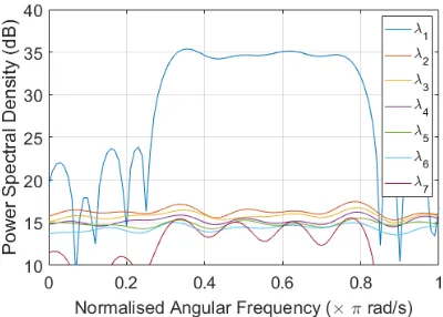
As mentioned in Section III, when strongly correlated sources are present, the dimension of the signal subspace does not coincide with the number of sources present. Figure 1 displays the power spectral density of the eigenvalues of the non-smoothed space-time covariance matrix. Only one eigenvalue is significant in magnitude, suggesting one source present.

The assumption that the steering vectors are part of the sig-nal subspace is still valid. However, as there are more sources than signal eigenvectors, the latter will contain a combination of the source steering vectors. Due to the Vandermonde structure of these steering vectors, no linear combination of these will result in a legitimate steering vector. This means that the true steering vectors will no longer be orthogonal to the noise subspace [2]. This is severely detrimental to the angular resolution of the PMUSIC algorithm. This loss of resolution can lead to knock-on effects as part of a larger system, such

Figure 1: PSD of polynomial eigenvalues of the non-smoothed space-time covariance matrix

as a decreased probability of detection in passive applications. Figure 2 displays the spatio-spectral estimation for the non-spatiality smoothed case. While there are noticeable spatial peaks around−40◦_and30◦_{, the peaks are wide (∼20}◦ _{1 dB}

width) and less than 5 dB in magnitude (relative to the floor).

Figure 2: SSP-MUSIC spatio-spectrum of 2 coherent sources

B. Spatially Smoothed SSP-MUSIC

As mentioned in Section IV, spatial smoothing will restore the rank of the source cross spectral density matrix providing the conditions K≥P, andL > P are met. In this particular scenario, the 7 element antenna array is split into 3 overlapping subarrays. This yields and effective array length of 5 -satisfying the above condition. Figure 3 displays the PSD of the polynomial eigenvalues. Two of which, have significant magnitude over the same wide bandwidth.

Figure 3: PSD of polynomial eigenvalues of the spatially smoothed covariance matrix

Figure 4: Spatially Smoothed SSP-MUSIC spatio-spectrum with 2 coherent sources present

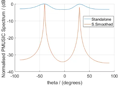
The spatially smoothed SSP-MUSIC algorithm produces a spatio spectrum with a much higher angular resolution, with a 1 dB peak width of ∼1◦_{. The spatial only characteristics}

of the spatially smoothed, and standalone versions of the SSP-MUSIC algorithm are displayed in Figure 5. This spatial only representation is determined via spectral averaging through the bandwidth of sources.

Figure 5: Normalised Angular spectrum comparing the SS and non-SS PMUSIC algorithms at Ω∈[0.3π,0.8π]

VII. CONCLUSION

Through the extension of a popular narrowband technique, this paper has introduced an improved variation of the poly-nomial MUSIC algorithm, providing a potential solution for the problem of broadband direction of arrival estimation in a multipath environment. The solution and proof proposed in this paper is a direct polynomial analogue of the narrowband case; demonstrating the power and elegance of polynomial matrix techniques and the PEVD for broadband antenna array signal processing.

Simulation results are presented to assess the performance gain of using this spatial smoothing technique for coherent broadband direction of arrival estimation in conjunction with the use of polynomial MUSIC algorithm. The non-smoothed PMUSIC algorithm encounters serious difficulties that are manifested as a loss of resolution in the presence of strongly correlated, or coherent sources. When the spatial smoothing technique is applied to the polynomial covariance matrix, the PMUSIC algorithm produces similar results to the case of uncorrelated sources, with a relatively modest loss of aperture.

ACKNOWLEDGEMENT

This work was supported by Leonardo Airborne and Space Systems.

REFERENCES

[1] R. Schmidt, “Multiple emitter location and signal parameter estimation,”

IEEE Trans. Antennas and Propagation, vol. 34, no. 3, pp. 276–280, Mar 1986.

[2] T.-J. Shan, M. Wax, and T. Kailath, “On spatial smoothing for direction-of-arrival estimation of coherent signals,” IEEE Trans. Acoustics, Speech, and Signal Processing, vol. 33, no. 4, pp. 806–811, Aug 1985. [3] G. Fabrizioet al., “Single site geolocation method for a linear array,”

in2012 IEEE Radar Conference, May 2012, pp. 885–890.

[4] J. G. McWhirter, P. D. Baxter, T. Cooper, S. Redif, and J. Foster, “An evd algorithm for para-hermitian polynomial matrices,” IEEE Trans. Signal Processing, vol. 55, no. 5, pp. 2158–2169, May 2007. [5] S. Redif, S. Weiss, and J. G. McWhirter, “Sequential matrix

diagonal-ization algorithms for polynomial evd of parahermitian matrices,”IEEE Trans. Signal Processing, vol. 63, no. 1, pp. 81–89, Jan 2015. [6] S. Redif, S. Weiss, and J. McWhirter, “Relevance of polynomial

matrix decompositions to broadband blind signal separation,” Signal Processing, vol. 134, pp. 76–86, 11 2016.

[7] M. A. Alrmah, S. Weiss, and S. Lambotharan, “An extension of the music algorithm to broadband scenarios using a polynomial eigenvalue decomposition,” in2011 EUSIPCO, Aug 2011, pp. 629–633. [8] M. A. Alrmah, “Broadband Angle of Arrival Estimation Using

Polyno-mial Matrix Decompositions,” Ph.D. dissertation, Univ. of Strathclyde, 2015.

[9] J. E. Evans, J. R. Johnson, and D. F. Sun, “Application of advanced signal processing techniques to angle of arrival estimation in atc navigation and surveillance system,” 1982.

[10] S. U. Pillai and B. H. Kwon, “Forward/backward spatial smoothing techniques for coherent signal identification,” IEEE Trans. Acoustics, Speech, and Signal Processing, vol. 37, no. 1, pp. 8–15, Jan 1989. [11] R. T. Williams, S. Prasad, A. K. Mahalanabis, and L. H. Sibul,

“An improved spatial smoothing technique for bearing estimation in a multipath environment,”IEEE Trans. Acoustics, Speech, and Signal Processing, vol. 36, no. 4, pp. 425–432, Apr 1988.

[12] M. Alrmah, S. Weiss, and J. McWhirter, “Implementation of accurate broadband steering vectors for broadband angle of arrival estimation,” inIET Int. Signal Processing Conf. 2013, Dec 2013, pp. 1–6. [13] J. Corr et al., “Multiple shift maximum element sequential matrix