City, University of London Institutional Repository
Citation: Spreeuw, J. (2006). Types of dependence and time-dependent association
between two lifetimes in single parameter copula models (Actuarial Research Paper No. 169). London, UK: Faculty of Actuarial Science & Insurance, City University London.This is the unspecified version of the paper.
This version of the publication may differ from the final published
version.
Permanent repository link: http://openaccess.city.ac.uk/2301/
Link to published version: Actuarial Research Paper No. 169
Copyright and reuse: City Research Online aims to make research
outputs of City, University of London available to a wider audience.
Copyright and Moral Rights remain with the author(s) and/or copyright
holders. URLs from City Research Online may be freely distributed and
linked to.
City Research Online: http://openaccess.city.ac.uk/ [email protected]
Faculty of Actuarial
Science
and
Statistics
Types of Dependence and
Time-dependent Association
between Two Lifetimes in
Single Parameter Copula
Models
Jaap Spreeuw
Actuarial Research Paper
No. 169
February 2006
ISBN 1 901615-96-0
Cass Business School
106
Bunhill
Row
London
EC1Y
8TZ
T +44 (0)20 7040 8470
www.cass.city.ac.uk
Types of dependence and time-dependent association between
two lifetimes in single parameter copula models
Jaap Spreeuw
January 31, 2006
Abstract
1
Introduction
Traditionally, it has been presumed in multiple life contingencies that the remaining lifetimes of the lives involved are mutually independent. As some empirical investigations have shown, for a married couple, this standard assumption is based on computational convenience rather than realism.
Over the past few years, several papers about insurance contracts on two lives have been published which allow for dependence between the two lifetimes. Frees et al. (1996) and Carriere (2000) present alternative ways of modeling dependence of times of death of coupled lives and applying them to a dataset. In both papers, a significant degree of positive correlation between lifetimes was observed. This implies, for instance, that joint life annuities are underpriced while last survivor annuities are overpriced. Carriere and Chan (1986) present boundaries of single premiums for last survivor annuities. All three papers adopt a methodology based on copulas, an approach which is popular nowadays. Other papers studying bounds of single premiums are Dhaene et al. (2000) and Denuit et al. (2001).
All these papers study the impact of dependency of two remaining lifetimes on the pricing of life insurance products on the lives concerned. Dependency, however, also affects the valuation of such contracts over time. Prospective provisions (also known as reserves) are based on laws of mortality which apply to the policy valuation date. If the remaining lifetimes of a couple are dependent at the outset of a policy, then any of the two lives’ survival probabilities may depend on the life status of the partner. Moreover, the joint distribution of remaining lifetimes, given the survival of both partners to a certain date, is affected as well. Using copula models to modify a formula used in the valuation of survivorship life insurance policies, Margus (2002) has pointed out that mortality rates of a life whose spouse is still alive differs from the mortality rates of a life whose spouse already died before the time of valuation. Youn et al. (2002) show that a lot of well-known relationships between probabilities and single premiums in multiple life contingencies are not valid in case of dependent lifetimes. They establish, however, that the validity of those relationships can be restored if the definition of individual survival probabilities allows for the life status of the partner. Carriere (2000), stating that the copula should affect the lives from the time of marriage, rather than from the time of birth, uses similar arguments. Moreover, it is not sufficient just to conclude that there is dependence between remaining life-times. It is also essential to state what type of dependence applies. Hougaard (2000) points out that within a time framework, one can basically distinguish between three different categories:
1. Instantaneous dependence: dependence caused by common events affecting both lives at the same time.
2. Long-term dependence: dependence which is caused by a common risk environment, af-fecting the surviving partner for their remaining lifetime.
3. Short-term dependence: the event of death of one life changes the mortality of the other life immediately, but this effect diminishes over time.
“broken heart syndrome” (as researched in Parkes et al., 1969, and Jagger and Sutton, 1991) is the most well-known example of short-term dependence.
It is a question which type of dependence prevails within the framework of multiple life contingencies. Hougaard (2000) suggests that in case of a married couple, short-term dependence is perhaps more relevant than long-term dependence. This assertion is underpinned by one of the main results from the empirical work in Parkes et al. (1969) and Jagger and Sutton (1991). Both studies show that within about 6 months after death of the partner, the mortality of widowers is comparable with that of married men. Youn and Shemyakin (1999, 2001) show that, when implementing a copula model, ignoring the difference between the physical ages of the two partners can lead to an underestimation of the instantaneous dependence and short-term dependence.
As long as both lives of a couple are alive, the degree of association between the respective remaining lifetimes depends on time. This gives rise to another question, namely which patterns of association over time between members of a couple are realistic. Moreno (1994) discusses this issue, also known as aging, in the context of frailty models, which are an important subclass of Archimedean copula models.
This paper analyzes the time-dependent association implied by copula models, and identifies their type of dependence. We assess the impact of the life history of one life on the mortality of the other life. If the one life has died before the other life, we will also distinguish between the different times of death. In this respect, our approach differs from the one in Margus (2002) who considers only one state “Dead” of the partner without specifying when the partner died. We also investigate how the dependence between the two lives will change over time, as long as they are both still alive. We consider one and the same couple at the outset and restrict our study in this paper to models with one parameter for dependence only.
We have developed a methodology which is based on analyzing the force of mortality of one life. Our paper sheds new light on theoretical properties of copulas. Besides, it gives an answer to the important question which copula models may be suitable for modelling dependence, which exhibits itself in the practice of the insurance of couples. Some of the copulas discussed in this contribution have not been widely studied before, and this has led to some interesting findings. Our approach helps the actuary to choose an appropriate copula and provides a framework for the calculation of provisions of contracts on two lives.
The organization of this paper is as follows. In Section 2, we specify the conditional marginal and joint survival functions which we want to analyze. Section 3 gives an introduction to copula models and outlines the structure for the next two sections. Section 4 concerns the previous death of one life and analyses the impact on the death of the other life, while Section 5 deals with the case where both lives are still alive. A numerical example about provisions of an insurance contract on two lives is given in Section 6. A discussion in Section 7 concludes the paper.
2
Conditional marginal and joint survival functions
We consider a contract effected on two lives(x)and (y), agedx andy, respectively at duration
0. The complete remaining lifetimes of (x)and(y) are denoted byTx andTy, respectively, with
marginal survival functions S1(s1) and S2(s2). We assume that Tx and Ty are continuously
distributed, with upper boundsωx−xandωy−y, respectively. The variablesωxandωy denote
the limiting ages of (x) and (y). The joint survival function is denoted by S(s1, s2).
We want to calculate the prospective provision at durationt≥0. We assume that the policy is in force if at least one of both lives is alive.
ty andty+dt, withty ∈[0, t]. Then the survival function of remaining lifetime of(x)at duration
t, given death of (y) at timety, is given by:
S1;t(s|Ty =ty) = P[Tx > t+s|Tx > t, Ty =ty] =
−dtdyP[Tx > t+s, Ty> ty]
−dtdyP[Tx > t, Ty > ty]
=
d
dtyS(t+s, ty)
d
dtyS(t, ty)
. (1)
Next, consider the case where both are still alive at duration t≥0. Then the survival function of remaining lifetime of (x) att, given survival of(y) to timet, is given by
S1;t(s|Ty > t) =P[Tx> t+s|Tx> t, Ty > t] =
P[Tx > t+s, Ty > t]
P[Tx> t, Ty > t]
= S(t+s, t)
S(t, t) . (2)
The expressions for S2;t(s|Tx=tx) and S2;t(s|Tx > t) are similar to (1) and (2), respectively,
withx andy interchanged. The joint survival function, given survival of both tot, is defined as
St(s1, s2) =P[Tx> t+s1, Ty > t+s2|Tx > t, Ty > t] =
S(t+s1, t+s2)
S(t, t) . (3)
3
Copula models
We start this section by giving a general introduction to copulas in Subsection 3.1. Then, we show how the equations established in Section 2 are specified if a copula model applies. We make a distinction between previous death of one life (Subsection 3.2) and survival of both (Subsection 3.3). Finally, in Subsection 3.4, we will give an overview of the copula families to be considered in this paper.
3.1
Introduction to general copulas
If we apply a copula model, the joint distribution is determined by the marginals and a copula function of two arguments, denoted by C[·,·]. Assuming that 0 ≤ u ≤ 1 and 0 ≤ v ≤ 1, this function has the following properties:
1. C[0, v] =C[u,0] = 0; 2. C[1, v] =v andC[u,1] =u;
3. C[·,·]is nondecreasing in each argument.
For an overview of applications of copulas in actuarial science, see Frees and Valdez (1998). In the sequel, we will use survival copulas only. Then the joint survival function is a survival copula function, with the marginal survival functions as its arguments:
S(s1, s2) =C[S1(s1), S2(s2)].
3.2
Previous death of one partner
For (1), we get:
S1;t(s|Ty =ty) =P[Tx > t+s|Tx > t, Ty =ty] =
(C2[S1(t+s), v])v=S2(ty)
(C2[S1(t), v])v=S2(ty)
, (4)
with C2[·,·] denoting the partial derivative of C[·,·] with respect to its second argument.
Ob-viously, this definition only makes sense if C2[S1(t), v]6= 0forv=S2(ty).
We prefer to specify the mortality in terms of the forces of mortality, rather than the sur-vival function, if possible. The advantage of this is the multiplicative relationship between this quantity and the related quantity applying to the case of independence. Provided that
(C2[S1(t+s), v])v=S2(ty)6= 0, the forces of mortality are given as:
µ1(x+t+s|Ty =ty) = −
d dsln
h
(C2[S1(t+s), v])v=S2(ty)
i
= µ1(x+t+s)S1(t+s) (C21[u, v])u=S1(t+s);v=S2(ty) (C2[S1(t+s), v])v=S2(ty)
, (5)
withµ1(x+t+s)denoting the force of mortality at agex+t+scorresponding to the distribution ofTx. FurthermoreC21[·,·]is the second derivative with respect to its second andfirst argument.
Another advantage of the force of mortality representation is that it allows us to adopt the concepts in Hougaard (2000). We will focus on the specification of conditional laws of mortality through forces of mortality and analyze their behavior as a function of ty, the time of death
of the partner. For several copulas, we will work out whether there is long-term or short-term dependence between the lives. Our method is strongly based on Hougaard’s definition, which follows below.
Definition 1 The remaining lifetimes Tx and Ty exhibit short-term dependence if
µ1(x+t+s|Ty =ty) is an increasing function of ty ∈[0, t](or alternatively, if
µ2(y+t+s|Tx =tx) is an increasing function of tx ∈ [0, t]). On the other hand, there is
long-term dependence between Tx and Ty if µ1(x+t+s|Ty =ty) is constant or decreasing as
a function of ty ∈[0, t] (or equivalently, if µ2(y+t+s|Tx =tx) is constant or decreasing as a
function of tx∈[0, t]).
As we will see below now, the case of a force of mortality which is constant as a function of the time of death does not exist in copula models. It follows from (5) that if the force of mortality of (x) is constant, then
C21[u, v]
C2[u, v]
=dln [C2[u, v]]
du , u, v∈[0,1],
is independent of v. This implies:
ln [C2[u, v]] =K1(u) +K2, (6)
with K1(u) denoting a real valued differentiable function, depending only on u and the
para-meters of dependence, and not on v. In (6),K2 is a real valued constant. This leads to
with K3 denoting another real valued constant. The condition C[u,0] = 0 foru∈[0,1] implies
K3 = 0. Then, the conditionC[u,1] =ufor all u∈[0,1]impliesK1(u) = ln [u]−K2. Hence,
C[u, v] =uv,
being the independence copula. In other words, if two lifetimes are dependent and a copula model applies, then the force of mortality of one life always depends on the time of death of the other life.
We will identify the type of dependence for some copula families, which is the topic of Section 4.
3.3
Both lives survive
Next, we consider the case of survival of both. Then, equation (2) becomes:
S1;t(s|Ty > t) = Pr [Tx> t+s|Tx> t, Ty > t] =
Pr [Tx> t+s, Ty > t]
Pr [Tx> t, Ty > t]
= C(S1(t+s), S2(t))
C(S1(t), S2(t))
.
(7) A similar relationship holds for S2;t(s|Ty > t) = Pr [Ty > t+s|Tx> t, Ty > t]:
S2;t(s|Tx > t) = Pr [Ty > t+s|Tx> t, Ty > t] =
Pr [Tx> t, Ty > t+s]
Pr [Tx> t, Ty > t]
= C(S1(t), S2(t+s))
C(S1(t), S2(t))
.
(8) Once again, whenever possible, we prefer to express the effect of survivorship of the partner through a force of mortality function. The force of mortality corresponding to survival function (7) is given by:
µ1(x+t+s|Ty > t) = −
d
dsln [C(S1(t+s), S2(t))]
= µ1(x+t+s)S1(t+s) (C1[u, v])u=S1(t+s);v=S2(t) C(S1(t+s), S2(t))
. (9)
Equation (3) becomes:
St(s1, s2) =Ct[S1;t(s1|Ty > t), S2;t(s2|Tx > t)] =
C[S1(t+s1), S2(t+s2)]
S(t, t) , (10)
determined by the marginalsS1;t(s|Ty > t) and S2;t(s|Tx> t) as well as a new copulaCt.
In Section 5, we derive the form of the copula Ct for some copula families. We assume that
t is such thatS(t, t)>0.
3.4
Copulas to be considered
In this paper, in both Sections 4 and 5, we will first of all discuss the three special cases of independence, comonotonicity (Fréchet upper bound) and countermonotonicity (Fréchet lower bound). This is followed by Archimedean copulas.
If the two lifetimes are independent, the copula is specified as C[u, v] = uv. The Fréchet upper bound gives maximal positive dependence, with C[u, v] = min [u, v]. On the other hand, the Fréchet lower bound represents maximal negative dependence, and we have C[u, v] = max [u+v−1,0].
More formally, we assume that the two lifetimes are Positive Quadrant Dependent (PQD in short). According to Lehmann (1966), this is the case if
Pr [Tx > s1, Ty > s2]≥Pr [Tx> s1] Pr [Ty > s2] ∀s1, s2 ∈R.
In general, it may not be easy to obtain straightforward expressions for the equations in the previous subsection. Archimedean copulas have been well known and widely applied for their mathematical tractability, as well as their flexibility, and will therefore be considered. An Archimedean copula is constructed by a generator, being a function φ(·) : [0,1] → R+ with
a continuous first and second derivative, denotingφ0(τ) and φ00(τ) respectively, satisfying φ(1) = 0, φ0(τ)<0 and φ00(τ)>0, 0≤τ ≤1,
for all τ ∈(0,1). Then the copula generated by the function φ(·) is expressed as C[u, v] =φ[−1](φ(u) +φ(v)), 0≤u, v≤1,
with φ[−1](·), being the pseudo-inverse function of φ(·):
φ[−1](τ) =
½
φ−1(τ), for 0≤τ ≤φ(0)
0, for φ(0)≤τ ≤ ∞.
In the above equation,φ−1(·)is the inverse function ofφ(·). The pseudo-inverse and the inverse function coincide completely if limτ↓0φ(τ) = ∞. If this property holds, the generator is said
to be strict. For the sake of mathematical convenience (to avoid technical complications with the specification of the force of mortality), we will only discuss Archimedean copulas with strict generators, hence
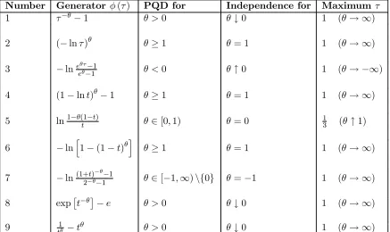
C[u, v] =φ−1(φ(u) +φ(v)), 0≤u, v≤1. (11) Archimedean copulas have been introduced in Genest and MacKay (1986a,1986b). For more details about Archimedean copulas and their properties, see Chapter 4 of Nelsen (1999). We will use some of the families described therein as illustrations. We only consider Archimedean copulas which allow for at least a range of Positive Quadrant Dependence and which explicitly contain the important special case of independence. In this paper, nine families are object of study. They are tabulated in Table 1.
Some of the copula types in this table have well known names. Families 1,2,3,5 and 6
Number Generator φ(τ) PQD for Independence for Maximum τ
1 τ−θ−1 θ >0 θ↓0 1 (θ→ ∞)
2 (−lnτ)θ θ≥1 θ= 1 1 (θ→ ∞)
3 −lneeθτθ−−11 θ <0 θ↑0 1 (θ→ −∞)
4 (1−lnt)θ−1 θ≥1 θ= 1 1 (θ→ ∞)
5 ln1−θ(1t−t) θ∈[0,1) θ= 0 13 (θ↑1)
6 −lnh1−(1−t)θi θ≥1 θ= 1 1 (θ→ ∞)
7 −ln(1+t)−
θ
−1
2−θ−1 θ∈[−1,∞)\{0} θ=−1 1 (θ→ ∞)
8 exp£t−θ¤−e θ >0 θ↓0 1 (θ→ ∞)
[image:11.595.75.512.130.390.2]9 t1θ −tθ θ >0 θ↓0 1 (θ→ ∞)
Table 1: Archimedean copula families
4
Copula models, one life died
4.1
Special cases
4.1.1 Independence
For C[u, v] =u v, (4) leads to
S1;t(s|Ty =ty) =
S1(t+s)
S1(t)
,
while (5) yields:
µ1(x+t+s|Ty =ty) =µ1(x+t+s)
S1(t+s)
S1(t+s)
=µ1(x+t+s),
which is as expected: the force of mortality of (x) is not affected at all by the time of death of
(y).
4.1.2 Fréchet upper bound
For C[u, v] = min [u, v], we have C2[u, v] = I{u>v}, so S1;t(s|Ty =ty) only exists if S2(ty) <
S1(t), in which case we get:
S1;t(s|Ty =ty) =
(
1 for s < S1[−1](S2(ty))−t
0 for s > S1[−1](S2(ty))−t
, (12)
defining
S1[−1](κ) =
½
S1−1(κ) for 0< κ≤1
ωx for κ= 0
In words, given death of (y) at ty, (x) dies with certainty at age x+ S1[−1](S2(ty)). Although
a force of mortality cannot be specified (since (12) is degenerate), this can be considered as an example of long term dependence: S1[−1](S2(ty))increases inty: the sooner(y) dies, the sooner
(x) dies. Note that if(y) dies at 0, then(x) dies at0.
4.1.3 Fréchet lower bound
For C[u, v] = max [u+v−1,0], we haveC2[u, v] =I{v>u−1}, so S1;t(s|Ty =ty) only exists if
S2(ty)>1−S1(t), which is always satisfied. In this case we get:
S1;t(s|Ty =ty) =
(
1 for s < S1[−1](1−S2(ty))−t
0 for s > S1[−1](1−S2(ty))−t
,
withS1[−1](·)as defined in (13). In other words, given death of(y)atty,(x)dies with certainty at
agex+S1−1(1−S2(ty)). The sooner(y)dies, the later(x)dies. Note thatS1;t(s|Ty =ty) =ωx
forty= 0: death of(y)at0implies death of(x)not before attaining the limiting age. As stated
in Margus (2002), the death of one life prevents the death of the other life.
4.2
Archimedean copulas
Substituting (11) into (5) leads to: µ1(x+t+s|Ty =ty)
= µ1(x+t+s)S1(t+s)
¡
−φ0(S1(t+s))
¢Ã
−
¡
φ−1¢00(v)
¡
φ−1¢0(v)
!
(v=φ(S(t+s,ty)))
. (14)
Note that, in this expression only the function
−
á
φ−1¢00(v)
¡
φ−1¢0(v)
!
(v=φ(S(t+s,ty)))
=−d
ln
∙
−³¡φ−1¢0(v)´
(v=φ(S(t+s,ty)))
¸
dv , (15)
depends onty. If this function decreases (increases) inty, then the dependence is of a long-term
(short-term) nature.
Our analyses establish that almost all of the copulas exhibit long term dependence. Thefirst four families listed in the table have a frailty specification. Frailty is a basic example of long term dependence. This has been pointed out in Hougaard (2000), and will be demonstrated here again.
Case 2 (Frailty) If the inverse of the generator is a Laplace transform, we have the general expression
φ−1(v) =
Z ∞
z=0
e−zvdF(z),
with F(z) denoting the c.d.f. of frailty. Then we have
¡
φ−1¢0(v) =
Z
ze−zvdF(z),
and
¡
φ−1¢00(v) =
Z
So d dty à − ¡
φ−1¢00(v)
¡
φ−1¢0(v)
!
(v=φ(S(t+s,ty)))
= φ0(S2(ty))S2(ty)µ(y+ty)
R
z3e−zvdF (z)R ze−zvdF(z)−¡R z2e−zvdF (z)¢2
¡R
ze−zvdF(z)¢2
≤ 0.
As thefirst illustration, we discuss the Clayton family. This type has some special properties, as we will see in this, as well as in next section. This is followed by the Gumbel-Hougaard copula (applied in Youn and Shemyakin (1999, 2001), Youn et al., 2002, and Denuit et al., 2001) and Frank’s copula (applied in Frees et al., 1996, Carriere, 2000, and Margus, 2002).
Example 3 (Clayton) The inverse of the generator, φ−1(τ) = (τ + 1)−1θ is the Laplace trans-form of the Gamma(α, β) distribution with parameters α = θ−1 and β = 1. In general the Laplace transform of a Gamma(α, β) distribution is φ−1(τ) =
³
τ β + 1
´−1
θ
, leading to a gen-erator φ(τ) = β¡t−θ−1¢. From Genest and MacKay (1986b), we know that a generator is determined up to a positive multiplier. Hence, the value of β does not affect the joint distribu-tion. Equation (14) gives:
µ1(x+t+s|Ty =ty) =µ1(x+t+s) (θ+ 1)
(S1(t+s))−θ
(S1(t+s))−θ+ (S2(ty))−θ−1
,
which is decreasing in ty. Note the special casety = 0(death immediately after issue), in which
case the above expression leads to:
µ1(x+t+s|Ty =ty) = (θ+ 1)µ1(x+t+s).
In other words, if (y) dies immediately after issue of a contract, the force of mortality (x) is
(θ+ 1) times the marginal force of mortality for any time in the future. We will discuss this feature further in Section 5 where Clayton’s copula is considered again.
Example 4 (Gumbel-Hougaard) The inverse of the generator, φ−1(τ) = exp³−τ1θ
´
is the Laplace transform of the positive stable distribution, as pointed out in Frees and Valdez (1998). Equation (14) gives:
µ1(x+t+s|Ty =ty) = µ1(x+t+s)
Ã
(−lnS1(t+s))θ
(−lnS1(t+s))θ+ (−lnS2(ty))θ
!1−1θ
µ
1 + (θ−1)
³
(−lnS1(t+s))θ+ (−lnS2(ty))θ
´−1
θ
¶ ,
which is decreasing as a value of ty.
Example 5 (Frank) The inverse of the generator, φ−1(τ) = ln£1 +¡eθ−1¢e−τ¤/θ is the Laplace transform of the logarithmic series distribution on the positive integers, as pointed out in Frees and Valdez (1998). Equation (14) gives:
µ1(x+t+s|Ty =ty) = µ1(x+t+s)S1(t+s) (−θ)
eθS1(t+s)
1−eθS1(t+s) Ã
1−eθ
(1−eθ)−¡1−eθS1(t+s)¢ ¡1−eθS2(ty)¢ !
which is decreasing as a value of ty.
A simple check with Mathematica shows that Family4 in Table 1 has a frailty specification as well, implying that dependence is also of a long term type. The frailty distribution involves a Bessel function. Families 5 to8 in Table 1 feature long term dependence as well. Only Family
9, has short term dependence in some cases, as will be shown below.
Example 6 (Family 9) The inverse of the generator is φ−1(τ) = 2−1θ
³
−τ +√4 +τ2´
1
θ . Equation (14) gives:
µ1(x+t+s|Ty =ty) = µ1(x+t+s)θ
Ã
1
S1(t+s)θ
−S1(t+s)θ
!
⎛
⎝w(t+s, ty) +
1
θ
q
4 + (w(t+s, ty))2
4 + (w(t+s, ty))2
⎞
⎠, (16)
with
w(t+s, ty) =
Ã
1
S1(t+s)θ
−S1(t+s)θ
!
+
Ã
1
S2(ty)θ
−S2(ty)θ
! .
For small ty and t+s, i.e. young ages and or short durations, (16) is increasing as a function
of ty. On the other hand, for larger values of ty and/ort+s, it is decreasing as a function of
ty.
5
Copula models, both survive
5.1
Special cases
5.1.1 Independence
For C[u, v] =u v, (9) leads to
µ1(x+t+s|Ty> t) =µ1(x+t+s),
which is as expected: in case of independence, the mortality of one life does not depend on the life history of the other life.
Furthermore, (10) leads to
St(s1, s2) =
S1(t+s)S2(t+s)
S(t, t) =S1;t(s|Ty > t)S1;t(s|Ty > t).
Hence, Ct(u, v) =uv: the joint distribution of remaining lifetime, given survival of both is the
independence copula again (as expected).
5.1.2 Fréchet upper bound
For C[u, v] = min [u, v], we have
S1;t(s|Ty > t) =
min [S1(t+s), S2(t)]
min [S1(t), S2(t)]
and a similar expression forS2;t(s|Ty > t). In this case, (10) leads to
Ct[S1;t(s|Ty > t), S2;t(s|Ty > t)] =
min [S1(t+s), S2(t+s)]
S(t, t)
= min [S1;t(s|Ty > t), S2;t(s|Ty > t)].
In words, if the joint distribution has the Fréchet upper bound as copula at the outset, it will continue to have the Fréchet upper bound as copula in the future.
5.1.3 Fréchet lower bound
For C[u, v] = max [u+v−1,0], we have
S1;t(s|Ty > t) =
max [S1(t+s) +S2(t)−1,0]
S(t, t) ,
and a similar expression forS2;t(s|Ty > t). In this case, (10) leads to
Ct[S1;t(s|Ty > t), S2;t(s|Ty > t)] =
max [S1(t+s) +S2(t+s)−1,0]
S(t, t)
= max [S1;t(s|Ty > t) +S2;t(s|Ty > t)−1,0].
In words, if the joint distribution has the Fréchet lower bound as copula at the outset, it will continue to have the Fréchet lower bound as copula in the future.
5.2
Archimedean copulas
We start this subsection by deriving the copula of the conditional joint survival function, given survival of both lives to a certain time in Subsubsection 5.2.1. Thereafter, in Subsubsection 5.2.2, we derive some time-dependent measures of association. Finally, in Subsubsection 5.2.3, we give some examples, extracted from Table 1.
5.2.1 Updated joint distribution
For Archimedean copulas, with the generator as defined in Subsection 3.4, the conditional mar-ginal survival function of remaining lifetime of (x), given survival of(x) and (y) to t, has the following expression:
S1;t(s|Ty > t) =
φ−1(φ(S1(t+s)) +φ(S2(t)))
S(t, t) , (17)
with a similar expression for S2;t(s|Tx> t). The force of mortality as defined in (9), is:
µ1(x+t+s|Ty > t)
= µ1(x+t+s) S1(t+s)
¡
−φ0(S1(t+s))
¢ Ã
−
¡
φ−1¢0(v)
¡
φ−1¢(v)
!
(v=φ(S(t+s,t)))
. (18)
Theorem 7 If the copula of a joint survival function copula at time0 is Archimedean, then the copula of the conditional joint survival function, given survival of both to t, is also Archimedean. Letφ(·)denote the generator of the copula at time0. Thenφt(·), the generator of the Archimedean copula at time t, is
φt(τ) =φ(τ ·S(t, t))−φ(S(t, t)), τ ∈[0,1]. (19)
Proof. We show that the joint distribution of remaining lifetime, given survival of both tot, comprises the copula generated byφt(·)in (19). Note,first of all thatφt(·)has all the properties of a generator for an Archimedean copula, namely φt(1) = 0, φ0t(τ) <0, and φ00t (τ) >0. The inverse of the generator φt(·), denoted by φ−t1(·), is
φ−t1(τ) = φ
−1(τ+φ(S(t, t)))
S(t, t) .
Applying (11), this leads to the updated copula, denoted byCt[·,·]:
Ct[u, v] =
φ−1(φ(u·S(t, t)) +φ(v·S(t, t))−φ(S(t, t)))
S(t, t) .
Substituting u=S1;t(s|Ty > t) and v=S2;t(s|Ty > t) gives, using expression (17)
Ct[S1;t(s|Ty > t), S2;t(s|Tx> t)] =
φ−1(φ(S1(t+s)) +φ(S2(t+s)))
S(t, t)
= Pr [Tx > t+s, Ty > t+s|Tx > t, Ty > t].
A similar result has been derived in Manatunga and Oakes (1996) in the context of the important subclass of frailty models.
Next, we consider the case of copula families which remains constant in time. They can be derived by solving the equation
φt(τ) =α(S(t, t))φ(τ), (21) forτ ∈[0,1]. The functionα(S(t, t))depends on S(t, t) only, and not onτ. In the Appendix, we prove that the solution of this equation is:
φ(v) = K
θ ³
v−θ−1´, θ∈R\ {0}, K≥0.
which is the generator of Clayton’s copula.
It is well known that Clayton’s copula implies association which is independent of time. Note, furthermore, that the Clayton family is the only type which satisfies this property.
In this subsection we use the notion of concordance ordering of copulas. A copula C(1) is smaller than C(2) if C(1)(u, v) ≤C(2)(u, v) for all u, v ∈[0,1]. For our analysis of the copulas
introduced in Subsection 3.4, we make use of some of the following theorems. The first one is from Nelsen (1999). The second one is due to Nelsen (1999) and is an extension of a result in Genest and MacKay (1986a). The last two have been derived in Genest and MacKay (1986a) and can also be found in Nelsen (1999). We define ωxy = min [t|S(t, t) = 0 ]as the limiting age
which the joint-life status can obtain.
Theorem 9 Let Ct1 and Ct2 be Archimedean copulas, generated, respectively, by φt1(·) and φt2(·). Assume both generators to be continuously differentiable on (0,1). Then ifφ0t1(·)/φ0t2(·)
is nondecreasing on (0,1), then Ct1 < Ct2.
Theorem 10 Let {Ct|t∈[0, ωxy]}, be a family of copulas with continuously differentiable
gen-erators φt(·). Then C = limt→ωxyCt is an Archimedean copula if and only if there exists a function in Ωsuch that for all s, τ in (0,1),
lim
t→ωxy
= φt(s)
φ0t(τ) =
φ(s)
φ0(τ). (22)
Theorem 11 Let {Ct|t∈[0, ωxy]}, be a family of copulas with differentiable generators φt(·)
in Ω. Then limt→ωxyCt (u, v) = min [u, v] if and only if,
lim
t→ωxy
= φt(τ)
φ0t(τ) = 0. (23)
Theorems 8 and 9 are used to investigate whether dependence has a monotone development (increasing or decreasing) over time. If dependence is decreasing, Theorem 10 can be used to
find the limiting form of dependence. For instance, ifφ(s)/φ0(τ) =tlns, then the limiting form is independence. On the other hand, if dependence is increasing, Theorem 11 can be used to check if maximal dependence is attained in the limit. Should this not be the case, then Theorem 10 could be applied to look for another limiting form. Note that we are actually dealing with two parameters in the copula, namelyθ and S(t, t), and we fixθ.
In each of the illustrating examples in Subsubsection 5.2.3 we derive the generator as a function of time.
5.2.2 Time-dependent measures of association
Several time-dependent measures of association have been developed in the literature. We discuss two which are related to Kendall’s tau, denoted by τ(Tx, Ty). It is defined as:
τ(Tx, Ty) = 4
Z 1
u=0
Z 1
v=0
C[u, v]dC[u, v] + 1. (24)
Kendall’s tau does not depend on the distribution of the marginals and this explains its pop-ularity. Independence, comonotonicity and countermonotonicity imply values for Kendall’s tau of 0,1 and −1, respectively.
From Genest and MacKay (1986a, 1986b), we know that for Archimedean copulas, (24) reduces to
τ(X1, X2) = 4
Z 1
u=0
φ(v)
φ0(v)dv+ 1. (25)
One measure of time-dependent association is Kendall’s tau pertaining to the copula constructed by the generator φt(τ), defined in (19). We will denote it by eτt(T1, T2). Hence
e
τt(Tx, Ty) = 4
Z 1
u=0
φt(v)
φ0t(v)dv+ 1 = 4
S(t, t)
Z 1
u=0
φ(u·S(t, t))−φ(S(t, t))
φ0t(u·S(t, t)) dv+ 1. (26)
The second measure to be discussed is the cross-ratio functionCR(S(t, t)), which has been introduced by Clayton (1978). Its characteristics are discussed in Oakes (1989). It is defined by Oakes as:
CR(S(t1, t2)) =
S(t1, t2)dtd1dtd2S(t1, t2)
d
dt1S(t1, t2)
d
dt2S(t1, t2)
. (27)
An interpretation of this quantity as an odds-ratio is given in Anderson et al. (1992). Some properties of the cross-ratio function are derived in Gupta (2003). Oakes also points out that
τt(Tx, Ty) =
CR(S(t1, t2))−1
CR(S(t1, t2)) + 1
, (28)
is a conditional version of Kendall’s tau.
For two reasons, we prefer the cross-ratio function to the truncated tau, as the degree of time-dependent association. First of all, an alternative definition of CR(·) is
CR(S(t1, t2)) =
µ1(x+t1|Ty =t2)
µ1(x+t1|Ty > t2)
. (29)
The interpretation is clear: it indicates the relative rate of increase of the force of mortality of the survivor at t1 upon death of the partner at t2.
Secondly, the cross-ratio function is easier to evaluate than the truncated tau, as no inte-gration is required. This is shown by dividing (14) by (18), using t2 =t1 =t =ty. This leads
to:
CR(S(t, t)) =
⎛ ⎜
⎝φ
−1(v)¡φ−1¢00(v)
³¡
φ−1¢0(v)´2
⎞ ⎟ ⎠
v=φ(S(t,t))
. (30)
In other words, the cross ratio function only depends on the inverse of the generator. This result has been derived in Oakes (1994).
Hougaard (2000) and Hougaard et al. (1992) have applied the cross-ratio function in the statistical analysis of twin data.
In each of the illustrating examples in Subsubsection 5.2.3, we will derive the cross-ratio function. Note that the papers introduced in this subsubsection focus on frailty models (being a subclass of Archimedean copulas) while this contribution deals with Archimedean copulas in general.
Some other measures of time-dependent association between two lives have appeared in the literature. Anderson et al. (1992) introduce the “Conditional expected residual life” and the “Conditional probability of survival”. Some of their properties have been derived in Gupta (2003). Bassan and Spizzichino (2001) introduce and discuss a bivariate aging function which can be used in the special case of exchangeable lifetimes (i.e. (x) and (y) have the same law of mortality).
5.2.3 Examples
First of all, we discuss the Clayton copula, followed by Gumbel-Hougaard and Frank.
Example 12 (Clayton) For φ(τ) =δ¡τ−θ−1¢, θ >0 and any δ >0, we have for (18):
µ1(x+t+s|Ty > t) =µ1(x+t+s)
(S1(t+s))−θ
(S1(t+s))−θ+ (S2(t))−θ−1
For (19), we have
φt(τ) =δ(S(t, t))−θ
³
τ−θ−1
´
=δ(S(t, t))−θφ(τ), (31)
so the copula essentially remains the same throughout time. It follows that the association remains the same as well. This is a confirmation of a previous result. The cross-ratio function is therefore constant in time, and equal to θ+ 1.
Example 13 (Gumbel-Hougaard) Forφ(τ) = (−ln [τ])θ, θ≥1, we have for (18):
µ1(x+t+s|Ty > t) =µ1(x+t+s)
Ã
(−lnS1(t+s))θ
(−lnS1(t+s))θ+ (−lnS2(t))θ
!1−1θ
. (32)
For (19), we have
φt(τ) = (−ln [τ S(t, t)])θ−(−ln [S(t, t)])θ. (33)
Using Theorem 9, we obtain that Ct < C and using Theorem 10, we find that the association
between the two lifetimes reduces to zero. In other words, the two lives become less dependent as they age. The cross-ratio function is:
CR((S(t, t))) = 1 + θ−1
−lnS(t, t). (34)
Example 14 (Frank) For φ(τ) =−ln£¡eθτ−1¢/¡eθ−1¢¤, we have for (18):
µ1(x+t+s|Ty > t)
= µ1(x+t+s)
¡
1−eθS2(t)¢eθS1(t+s)(−θ)S
1(t+s)
¡
(eθ−1) +¡eθS1(t+s)−1¢ ¡eθS2(t)−1¢¢ln
∙
1 +(e
θS1(t+s)−1)(eθS2(t)−1)
eθ−1
¸. (35)
For (19), we have
φt(τ) =−lne
θS(t,t)τ
−1
eθS(t,t)−1. (36)
One can see from this expression that the copula pertaining to time belongs to the Frank family as well with parameterθ updated toθ·S(t, t). As time proceeds, the parameter approaches zero, implying independence. The cross-ratio function is:
CR(S(t, t)) =− θS(t, t)
1−eθS(t,t). (37)
Most copulas give a decreasing dependence over time leading to independence as t approaches ωxy. Families8 and 9 of Table 1 are the only types where dependence is increasing over time.
Family 8will be treated below.
Example 15 (Family 8 of Table 1) If φ(τ) = exp¡t−θ¢−e, θ ≥ 1, then the inverse is
φ−1(τ) = (ln [τ+e])−1θ. we have for (18):
µ1(x+t+s|Ty > t)
= µ1(x+t+s) S1(t+s)
−θ
ln
h
exp
h
S1(t+s)−θ
i
+ exp
h
S2(ty)−θ
i
−e i
exphS1(t+s)−θ
i
exphS1(t+s)−θ
i
+ exphS2(ty)−θ
i
−e
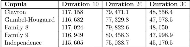
Copula Duration 10 Duration 20 Duration 30
Clayton 117,158 79,471.1 48,556.4
Gumbel-Hougaard 116,682 77,329.8 47,973.5
Family8 117,024 79,822.6 48,650
Family9 116,949 80,458.3 47,998.9
[image:20.595.126.457.129.212.2]Independence 115,605 75,038.7 45,170.5
Table 2: Provisions if (y) is still alive
For (19), we have
φt(τ) =
exph(τ ·S(t, t))−θi−exph(S(t, t))−θi
S(t, t) . (39)
Using Theorem 9, we obtain that Ct > C and using Theorem 11, we find that the association
between the two lifetimes increases to comonotonicity. In other words, the two lives become more dependent as they age. The cross-ratio function is
CR(S(t, t)) = 1 +θ³1 + [S(t, t)]−θ´. (40)
6
Numerical example
We consider a policy taken out by a couple where (x) = (y) = 60. The policy secures various benefits, one of which is a whole-life annuity due of10,000p.a., payable on life (x) while alive, independent of the life status of (y). These benefits are payable by single premium, which is
156,309(irrespective of the degree of association, as(x)and(y)are coupled by the copula upon issue). The marginals S1(·) and S2(·) are specified by the British life tables PMA92C20 and
PFA92C20, respectively. We assume that deaths are uniformly distributed between consecutive integer ages. Interest is at 4%p.a..
As copulas, we choose:
1. Clayton (long-term dependence, association constant over time);
2. Gumbel-Hougaard (long-term dependence, association decreasing in time); 3. Family 8(long-term dependence, association increasing in time);
4. Family 9(partially short-term dependence, association increasing in time);
For each copula, the parameter corresponds to a value of Kendall’sτ equal to 0.5at the outset. We calculate the provisions at durations10,20 and30. Table 2 shows the provisions that apply if(y) is still alive on the valuation date. Obviously these provisions are higher than in the case of independence.
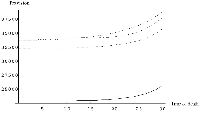
Figure 1 displays the curves for duration10. For Clayton, Gumbel-Hougaard, and Family8, the provisions are increasing as a function ofty, the time-of-death of(y). Since all these copulas
feature long-term dependence, this is not a very surprising result. The more distant the time of death of the partner, the higher the mortality of the remaining life, and hence the smaller the provisions. The provisions relating to Family9are slightly decreasing inty (from about109,150
forty = 0to108,900forty = 10), reflecting the short-term dependence for short durations. The
2 4 6 8 1 0
Time of death
6 0 0 0 0 7 0 0 0 0 8 0 0 0 0 9 0 0 0 0 1 0 0 0 0 0 1 1 0 0 0 0
[image:21.595.123.465.180.364.2]Provision
Figure 1: Provision at duration 10 as a function of the time of death of (y). (Gumbel-Hougaard: dashed-dotted; Clayton: solid; Family 8: dashed; Family9: dotted).
5 1 0 1 5 2 0 Time of death
5 0 0 0 0 5 5 0 0 0 6 0 0 0 0 6 5 0 0 0
Provision
[image:21.595.122.466.510.699.2]5 1 0 1 5 2 0 2 5 3 0
Time of death
2 5 0 0 0 2 7 5 0 0 3 0 0 0 0 3 2 5 0 0 3 5 0 0 0 3 7 5 0 0
[image:22.595.121.465.140.340.2]Provision
Figure 3: Provision at duration30as a function of the time of death of(y). (Clayton: solid; Family8:
dashed; Family9: dotted; Gumbel-Hougaard: dashed-dotted ).
9 (now slightly increasing as a function of ty) gives the largest provisions, followed by Family
8. Now it is Clayton giving minimal values. Figure 3 gives the provisions at duration 30. Now Gumbel-Hougaard and Family 9 display the largest values, while the provisions corresponding to Clayton’s copula are still minimal. We have done a similar exercise regarding provisions to be kept if the female annuitant is alive and the male has died, again for Kendall’sτ equal to0.5. In that case the graphs look a bit different. We have also done investigations based on smaller and larger values of Kendall’s coefficient of concordance. Different patterns arise for different cases, and the sizes of the provisions are by no means ordered, in the sense that e.g. Family
9 and Gumbel-Hougaard always give maximal values and minimal values for the provisions. The provisions produced from Gumbel-Hougaard’s copula become relatively larger compared to other copulas as the duration goes up, while relatively low values result from Clayton’s copula. It is difficult to explain all the features arising. This example, however, mainly serves to illustrate that provisions can differ substantially for different copulas, even if the association at the outset is the same. This implies that a copula should be chosen with care. Probably the results will differ for different combinations of ages at issue.
7
Discussion
In this paper, we have derived the type of association, as well as the aging properties, of some single parameter dependence models.
If two lifetimes are independent at the outset, then the time of death of one life has no impact at all on the mortality of the other life. Moreover, the conditional remaining lifetimes, given survival of both to a certain time, will remain independent. These results are easily understood by intuitive reasoning.
independence. We conclude that for all the copulas studied, there is no one which incorporates pure short-term dependence.
The question is whether this is realistic within the framework of married couples. Jagger & Sutton (1991) and Parkes et al. (1969) have shown that in most empirical studies the mortality of widowers increases sharply after death of their spouse, but returns to normal levels within a period of about six months. Hougaard (2000) suggests that for married couples, short-term dependence is probably more relevant than long-term dependence, and that for twins, probably the opposite holds. Firstly, contrary to twins, married couples do not have common genes, but only share their living environment. Secondly, the broken heart syndrome is a more significant feature among married couples than it is among twins. The applications carried out in Hougaard (2000), Hougaard et al. (1992) and Anderson et al. (1992) are all based on twin data.
Probably both the long term and the short term dependence effects merit separate para-meters, so single parameter models may be too limited to capture all the types of dependence featured. This is a topic for future research.
Furthermore, we have investigated the aging properties of some Archimedean copula models. We have established that in most cases the association between lifetimes decreases over time. In other words, individuals become less dependent as they age. Moreno (1994), devoting a discussion to aging in some frailty models, suggests that this pattern is intuitively desirable. His reasoning is that “if two lives have died, their survival experiences become independent of each other”. He uses the frailty distributions of Inverse Gaussian and a multiple point distribution as illustrations. Moreno argues that increasing dependence can occur if the mortality of some couples is extremely low, which is the case for Poisson distributed frailty.
These arguments may make sense if dependence is of a distinct long term nature, as specified by frailty models. For married couples, the assumption that dependence will diminish over time, seems stark. A young individual who is still engaged in paid employment will usually have a more extensive social network than a retiree, and hence better able to handle the shock of death of the partner. Moreover, youngsters have more opportunities to remarry. If an individual has been married for a long while, the shock of death of the spouse may have more dramatic (emotional) effects than for a life who has only got a partner for a couple of years.
This all gives arguments to use more sophisticated models to describe dependence, by al-lowing for short term dependence, as well as instantaneous dependence. Youn and Shemyakin (1999, 2001) have captured these two types of dependence by classifying individuals according to the age difference between the female and the male member of each couple. However, given any age difference, they use the Gumbel-Hougaard copula to specify the dependence between the lifetimes. As we have seen in this paper, using this copula implies assuming that there is long-term dependence and association is decreasing as both lives age.
References
[1] Anderson, J.E., Louis, T.A., Holm, N.V. and Harvald, B. (1992). Time-dependent asso-ciation measures for bivariate survival distributions. J. Americ. Statist. Assoc., 87 (419), 641-650.
[2] Bassan, B. and Spizzichino, F. (2001). Dependence and multivariate aging: the role of level sets of the survival function. In: System and Bayesian Reliability, Eds. Y. Hayakawa, T. Irony, M. Xie (World Scientific, River Edge, 2001), 229-242.
[4] Carriere, J.F. and Chan, L.K. (1986). The bounds of bivariate distributions that limit the value of last-survivor annuities. Transactions of the Society of Actuaries XXXVIII, 51-74. [5] Clayton, D.G. (1978). A model for association in bivariate life tables and its application
in epidemiological studies of familial tendency in chronic disease incidence. Biometrika 65, 141-151.
[6] Denuit, M., Dhaene, J., Le Bailly de Tilleghem, C. and Teghem, S. (2001). Measuring the impact of dependence among insured lifelengths. Belgian Actuarial Bulletin, 1 (1), 18-39. [7] Dhaene, J., Vanneste, M. and Wolthuis, H. (2000). A note on dependencies in multiple life
statuses. Mitteilungen der Schweizerisher Aktuarvereinigung, 19-33.
[8] Frees, E.W., Carriere, J.F. and Valdez, E.A. (1996). Annuity valuation with dependent mortality. Journal of Risk and Insurance, 63 (2), 229-261.
[9] Frees, E.W. and Valdez, E.A. (1998). Understanding relationships using copulas. N. Am. Actuar.J. 2, 1-25.
[10] Genest, C. and MacKay, R.J. (1986a). Copules archimédiennes et familles de lois bidimen-sionelles dont les marges sont données. Canad. J. Statist. 14 (2), 145-159.
[11] Genest, C. and MacKay, R.J. (1986b). The joy of copulas: bivariate distributions with uniform marginals. Amer. Statist. 40 (4), 280-283.
[12] Gupta, R.C. (2003). On some association measures in bivariate distributions and their relationships. Journal Statist. Plann. Inference 117, 83-98.
[13] Hougaard, P. (2000). Analysis of Multivariate Survival Data. Springer.
[14] Hougaard, P., Harvald, B. and Holm, N.V. (1992). Measuring the similarities between the lifetimes of adult Danish twins born between 1881-1930. J. Americ. Statist. Assoc. 87, 17-24. [15] Jagger, C. and Sutton, C.J. (1991). Death after marital bereavement - is the risk increased?
Statistics in Medicine 10, 395-404.
[16] Lehmann, E.L. (1966). Some concepts of dependence. Annals of Mathematical Statistics 37, 1137-1153.
[17] Manatunga, A.K. and Oakes, D. (1996). A measure of association for bivariate frailty distributions. J. Multivariate Anal. 56, 60-74.
[18] Margus, P. (2002) Generalized Frasier claim rates under survivorship life insurance policies. N. Am. Actuar. J. 6, 76-94.
[19] Moreno, L. (1994). Frailty selection in bivariate survival models: a cautionary note. Math. Popul. Stud., 4 (4), 225-233.
[20] Nelsen, R.B. (1999). An Introduction to Copulas, Lecture Notes in Statistics 139, Springer Verlag.
[21] Oakes, D. (1989). Bivariate survival models induced by frailties. J. Americ. Statist. Assoc., 84 (406), 487-493.
[23] Parkes, C.M., Benjamin, B. and Fitzgerald, R.G. (1969). Broken heart: a statistical study of increased mortality among widowers. British Medical Journal, 740-743.
[24] Youn, H. and Shemyakin, A. (1999). Statistical aspects of joint life insurance pricing. 1999 Proceedings of the Business and Statistics Section of the American Statistical Association, 34-38.
[25] Youn, H. and Shemyakin, A. (2001). Pricing practices for joint last survivor insurance. Actuarial Research Clearing House, 2001.1.
[26] Youn, H., Shemyakin, A. and Herman, E. (2002). A re-examination of the joint life mortality functions. N. Am. Actuar. J. 6, 166-170.
A
Proof in Subsubsection 5.2.1
In this Appendix, we solve the equation (21), namely
φt(τ) =α(S(t, t))φ(τ), (41) forφ(τ). Taking derivatives of both sides with respect toτ gives
α(S(t, t)) = S(t, t)φ
0(S(t, t)·τ)
φ0(τ) . (42)
We take the derivative of both sides with respect to τ again, and establish that the following relationship must hold:
S(t, t)φ00(S(t, t)·τ)
φ0(S(t, t)·τ) =
φ00(τ)
φ0(τ). (43)
Hence, the right hand side of the above equation does not depend on S(t, t). Taking the derivative of both with respect toS(t, t)gives the following differential equation forv=S(t, t)·τ:
¡
v·φ000(v) +φ00(v)¢φ0(v)−v£φ00(v)¤2= 0. (44) This differential equation is solved by
φ(v) = K2 1 +K1
v1+K1 +K
3, (45)
for some real valued constants K1, K2, andK3. The conditions φ0(v)<0 and φ00(v)>0 give
K2 < 0 and K1 < 0. Furthermore, the condition φ(1) = 0 gives K3 = −1+KK21. The final
condition limv↓0φ(v) =∞ leads toK1<−1. Substitutingθ=−(1 +K1), we get
φ(v) =−K2
θ ³
v−θ−1
´
, (46)
1
FACULTY OF ACTUARIAL SCIENCE AND STATISTICS
Actuarial Research Papers since 2001
Report
Number
Date Publication
Title
Author
135. February 2001. On the Forecasting of Mortality Reduction Factors.
ISBN 1 901615 56 1
Steven Haberman Arthur E. Renshaw
136. February 2001. Multiple State Models, Simulation and Insurer Insolvency. ISBN 1 901615 57 X
Steve Haberman Zoltan Butt Ben Rickayzen
137. September 2001 A Cash-Flow Approach to Pension Funding.
ISBN 1 901615 58 8
M. Zaki Khorasanee
138. November 2001 Addendum to “Analytic and Bootstrap Estimates of
Prediction Errors in Claims Reserving”. ISBN 1 901615 59 6
Peter D. England
139. November 2001 A Bayesian Generalised Linear Model for the
Bornhuetter-Ferguson Method of Claims Reserving. ISBN 1 901615 62 6
Richard J. Verrall
140. January 2002 Lee-Carter Mortality Forecasting, a Parallel GLM
Approach, England and Wales Mortality Projections.
ISBN 1 901615 63 4
Arthur E.Renshaw Steven Haberman.
141. January 2002 Valuation of Guaranteed Annuity Conversion Options.
ISBN 1 901615 64 2
Laura Ballotta Steven Haberman
142. April 2002 Application of Frailty-Based Mortality Models to Insurance
Data. ISBN 1 901615 65 0
Zoltan Butt Steven Haberman
143. Available 2003 Optimal Premium Pricing in Motor Insurance: A Discrete
Approximation.
Russell J. Gerrard Celia Glass
144. December 2002 The Neighbourhood Health Economy. A Systematic
Approach to the Examination of Health and Social Risks at Neighbourhood Level. ISBN 1 901615 66 9
Les Mayhew
145. January 2003 The Fair Valuation Problem of Guaranteed Annuity
Options : The Stochastic Mortality Environment Case.
ISBN 1 901615 67 7
Laura Ballotta Steven Haberman
146. February 2003 Modelling and Valuation of Guarantees in With-Profit and
Unitised With-Profit Life Insurance Contracts.
ISBN 1 901615 68 5
Steven Haberman Laura Ballotta Nan Want
147. March 2003. Optimal Retention Levels, Given the Joint Survival of Cedent and Reinsurer. ISBN 1 901615 69 3
Z. G. Ignatov Z.G., V.Kaishev
R.S. Krachunov
148. March 2003. Efficient Asset Valuation Methods for Pension Plans.
ISBN1 901615707 M. Iqbal Owadally
149. March 2003 Pension Funding and the Actuarial Assumption
Concerning Investment Returns. ISBN 1 901615 71 5
M. Iqbal Owadally
2
150. Available August
2004
Finite time Ruin Probabilities for Continuous Claims Severities
D. Dimitrova Z. Ignatov V. Kaishev
151. August 2004 Application of Stochastic Methods in the Valuation of
Social Security Pension Schemes. ISBN 1 901615 72 3
Subramaniam Iyer
152. October 2003. Guarantees in with-profit and Unitized with profit Life Insurance Contracts; Fair Valuation Problem in Presence of the Default Option1. ISBN 1-901615-73-1
Laura Ballotta Steven Haberman Nan Wang
153. December 2003 Lee-Carter Mortality Forecasting Incorporating Bivariate Time Series. ISBN 1-901615-75-8
Arthur E. Renshaw Steven Haberman
154. March 2004. Operational Risk with Bayesian Networks Modelling.
ISBN 1-901615-76-6
Robert G. Cowell Yuen Y, Khuen Richard J. Verrall
155. March 2004. The Income Drawdown Option: Quadratic Loss.
ISBN 1 901615 7 4
Russell Gerrard Steven Haberman Bjorn Hojgarrd Elena Vigna
156. April 2004 An International Comparison of Long-Term Care
Arrangements. An Investigation into the Equity, Efficiency and sustainability of the Long-Term Care Systems in Germany, Japan, Sweden, the United Kingdom and the United States. ISBN 1 901615 78 2
Martin Karlsson Les Mayhew Robert Plumb Ben D. Rickayzen
157. June 2004 Alternative Framework for the Fair Valuation of
Participating Life Insurance Contracts. ISBN 1901615-79-0
Laura Ballotta
158. July 2004. An Asset Allocation Strategy for a Risk Reserve
considering both Risk and Profit. ISBN 1 901615-80-4
Nan Wang
159. December 2004 Upper and Lower Bounds of Present Value Distributions
of Life Insurance Contracts with Disability Related Benefits. ISBN 1 901615-83-9
Jaap Spreeuw
160. January 2005 Mortality Reduction Factors Incorporating Cohort Effects.
ISBN 1 90161584 7
Arthur E. Renshaw Steven Haberman
161. February 2005 The Management of De-Cumulation Risks in a Defined
Contribution Environment. ISBN 1 901615 85 5.
Russell J. Gerrard Steven Haberman Elena Vigna
162. May 2005 The IASB Insurance Project for Life Insurance Contracts:
Impart on Reserving Methods and Solvency Requirements. ISBN 1-901615 86 3.
Laura Ballotta Giorgia Esposito Steven Haberman
163. September 2005 Asymptotic and Numerical Analysis of the Optimal
Investment Strategy for an Insurer. ISBN 1-901615-88-X
Paul Emms Steven Haberman
164. October 2005. Modelling the Joint Distribution of Competing Risks Survival Times using Copula Functions. I SBN 1-901615-89-8
Vladimir Kaishev Dimitrina S, Dimitrova Steven Haberman
165. November 2005.
Excess of Loss Reinsurance Under Joint Survival Optimality. ISBN1-901615-90-1
Vladimir K. Kaishev Dimitrina S. Dimitrova
166. November 2005.
Lee-Carter Goes Risk-Neutral. An Application to the Italian Annuity Market.
ISBN 1-901615-91-X
3
167. November 2005 Lee-Carter Mortality Forecasting: Application to the Italian Population. ISBN 1-901615-93-6
Steven Haberman Maria Russolillo
168. February 2006 The Probationary Period as a Screening Device:
Competitive Markets. ISBN 1-901615-95-2
Jaap Spreeuw Martin Karlsson
169. February 2006 Types of Dependence and Time-dependent Association
between Two Lifetimes in Single Parameter Copula Models. ISBN 1-901615-96-0
Jaap Spreeuw
Statistical Research Papers
Report
Number
Date
Publication Title
Author
1. December 1995. Some Results on the Derivatives of Matrix Functions. ISBN 1 874 770 83 2
P. Sebastiani
2. March 1996 Coherent Criteria for Optimal Experimental Design.
ISBN 1 874 770 86 7
A.P. Dawid P. Sebastiani
3. March 1996 Maximum Entropy Sampling and Optimal Bayesian Experimental Design. ISBN 1 874 770 87 5
P. Sebastiani H.P. Wynn
4. May 1996 A Note on D-optimal Designs for a Logistic Regression Model. ISBN 1 874 770 92 1
P. Sebastiani R. Settimi
5. August 1996 First-order Optimal Designs for Non Linear Models.
ISBN 1 874 770 95 6
P. Sebastiani R. Settimi
6. September 1996 A Business Process Approach to Maintenance: Measurement, Decision and Control. ISBN 1 874 770 96 4
Martin J. Newby
7. September 1996.
Moments and Generating Functions for the Absorption Distribution and its Negative Binomial Analogue. ISBN 1 874 770 97 2
Martin J. Newby
8. November 1996. Mixture Reduction via Predictive Scores. ISBN 1 874 770 98 0 Robert G. Cowell.
9. March 1997. Robust Parameter Learning in Bayesian Networks with Missing Data.ISBN 1 901615 00 6
P.Sebastiani M. Ramoni
10. March 1997. Guidelines for Corrective Replacement Based on Low Stochastic Structure Assumptions. ISBN 1 901615 01 4.
M.J. Newby F.P.A. Coolen
11. March 1997 Approximations for the Absorption Distribution and its Negative Binomial Analogue. ISBN 1 901615 02 2
Martin J. Newby
12. June 1997 The Use of Exogenous Knowledge to Learn Bayesian Networks from Incomplete Databases. ISBN 1 901615 10 3
M. Ramoni P. Sebastiani
13. June 1997 Learning Bayesian Networks from Incomplete Databases.
ISBN 1 901615 11 1
M. Ramoni P.Sebastiani
14. June 1997 Risk Based Optimal Designs. ISBN 1 901615 13 8 P.Sebastiani
H.P. Wynn
15. June 1997. Sampling without Replacement in Junction Trees.
ISBN 1 901615 14 6
Robert G. Cowell
16. July 1997 Optimal Overhaul Intervals with Imperfect Inspection and Repair. ISBN 1 901615 15 4
Richard A. Dagg Martin J. Newby
17. October 1997 Bayesian Experimental Design and Shannon Information.
ISBN 1 901615 17 0
P. Sebastiani. H.P. Wynn
18. November 1997. A Characterisation of Phase Type Distributions.
ISBN 1 901615 18 9
4
19. December 1997 A Comparison of Models for Probability of Detection (POD) Curves. ISBN 1 901615 21 9
Wolstenholme L.C
20. February 1999. Parameter Learning from Incomplete Data Using Maximum Entropy I: Principles. ISBN 1 901615 37 5
Robert G. Cowell
21. November 1999 Parameter Learning from Incomplete Data Using Maximum Entropy II: Application to Bayesian Networks. ISBN 1 901615 40 5
Robert G. Cowell
22. March 2001 FINEX : Forensic Identification by Network Expert Systems. ISBN 1 901615 60X
Robert G.Cowell
23. March 2001. Wren Learning Bayesian Networks from Data, using Conditional Independence Tests is Equivalant to a Scoring Metric ISBN 1 901615 61 8
Robert G Cowell
24. August 2004 Automatic, Computer Aided Geometric Design of Free-Knot, Regression Splines. ISBN 1-901615-81-2
Vladimir K Kaishev, Dimitrina S.Dimitrova, Steven Haberman Richard J. Verrall
25. December 2004 Identification and Separation of DNA Mixtures Using Peak Area Information. ISBN 1-901615-82-0
R.G.Cowell S.L.Lauritzen J Mortera,
26. November 2005. The Quest for a Donor : Probability Based Methods Offer Help. ISBN 1-90161592-8
P.F.Mostad T. Egeland., R.G. Cowell V. Bosnes Ø. Braaten
27. February 2006 Identification and Separation of DNA Mixtures Using Peak Area Information. (Updated Version of Research Report Number 25). ISBN 1-901615-94-4