Bayesian system identification of a nonlinear dynamical system using a novel variant of Simulated Annealing

Bayesian system identification of a nonlinear dynamical

system using a novel variant of Simulated Annealing

P.L. Green

Department of Mechanical Engineering, University of Sheffield, Mappin Street, Sheffield S1 3JD, United Kingdom

a r t i c l e i n f o

Article history: Received 28 March 2013 Received in revised form 20 March 2014 Accepted 9 July 2014 Available online 4 August 2014

Keywords:

Bayesian model updating Nonlinear system identification Markov chain Monte Carlo Simulated Annealing Deviance Information Criterion

a b s t r a c t

This work details the Bayesian identification of a nonlinear dynamical system using a novel MCMC algorithm:‘Data Annealing’. Data Annealing is similar to Simulated Anneal-ing in that it allows the Markov chain to easily clear‘local traps’in the target distribution. To achieve this, training data is fed into the likelihood such that its influence over the posterior is introduced gradually - this allows the annealing procedure to be conducted with reduced computational expense. Additionally, Data Annealing uses a proposal distribution which allows it to conduct a local search accompanied by occasional long jumps, reducing the chance that it will become stuck in local traps. Here it is used to identify an experimental nonlinear system. The resulting Markov chains are used to approximate the covariance matrices of the parameters in a set of competing models before the issue of model selection is tackled using the Deviance Information Criterion.

&2014 The Author. Published by Elsevier Ltd. This is an open access article under the CC BY license (http://creativecommons.org/licenses/by/3.0/).

1. Introduction

This paper is concerned with the system identification of a nonlinear dynamical system using experimentally obtained training data. A probabilistic, Bayesian approach is utilised throughout. Such an approach is now well established in the structural dynamics community – relatively recent advances include the use of Bayesian methods in structural health monitoring[1], modal identification[2], state-estimation[3](through use of the particle filter), the sensitivity analysis of large bifurcating nonlinear models[4]as well as an interesting study investigating the relations between frequentist and Bayesian approaches to probabilistic parameter estimation[5].

The identification problem detailed herein is one of model selectionas well asparameter estimation such that, using experimental dataD, one must endeavor to find the optimum modelMfrom a set of competing model structures as well as estimate the parameter vector

θ

of that particular model. Using Bayes' theorem a measure of the plausibility of a parameter vector

θ

, given experimental dataDand assumed model structureM, is given by

Pð

_θ

jD;MÞ ¼PðDj

θ

;MÞPð

θ

jMÞ

PðDjMÞ ð1Þ

wherePð

_θ

jD;MÞis the posterior probability density function (PDF) which one wishes to evaluate,PðDj

_θ

;MÞis termed the likelihood,Pð

_θ

jMÞ the prior andPðDjMÞ the evidence. The likelihood represents the probability that the experimental training data_Dwas witnessed according to the model_Mwith parameters

θ

. Defining the likelihood requires the selection

Contents lists available atScienceDirect

journal homepage:www.elsevier.com/locate/ymssp

Mechanical Systems and Signal Processing

http://dx.doi.org/10.1016/j.ymssp.2014.07.010

0888-3270&2014 The Author. Published by Elsevier Ltd. This is an open access article under the CC BY license (http://creativecommons.org/licenses/by/3.0/).

of an error-prediction model which describes the uncertainties present in the measurement and modelling processes (see

[6]for a detailed discussion of error-prediction models). The prior is a PDF which represents one's parameter estimates for modelMbefore the training data was known. The evidence is a normalising constant which ensures that the posterior PDF integrates to one.

This paper makes two main contributions. Firstly, a novel variant of Simulated Annealing (referred to as Data Annealing) is proposed and applied to a real system identification problem. It is shown to be computationally cheap and easy to tune. Secondly, it is shown that the issue of model selection of a real nonlinear dynamical system can be addressed using the Deviance Information Criterion (DIC). For the sake of readability the remainder of the introduction is split into two sections. The first outlines the motivation for the Data Annealing algorithm while the second focuses on the issue of model selection.

1.1. Motivation for the data annealing algorithm

For the case where one is attempting to identifyNDparameters (such that

θ

ARND), the evidence is given by

PðDjMÞ ¼Z ⋯Z PðDj

_θ

;MÞPð

_θ

jMÞd

θ

1⋯d

θ

ND: ð2Þ

This integral is usually intractable and its multidimensional nature makes it too computationally expensive to evaluate numerically (ifND42). Relatively early papers such as[7]made use of the property that themaximum a posteriori(MAP) parameter vector remains the same regardless of whether the posterior distribution has been normalised such that, through locating the MAP, a Taylor series expansion of the log posterior could be used to approximate the posterior PDF as a Gaussian.1Since then, an increase in computing power has allowed the adoption of Markov chain Monte Carlo (MCMC) methods. These involve the creation of an ergodic Markov chain whose stationary distribution is equal to the posterior PDF such that, once converged, the Markov chain is generating samples fromPð

_θ

jD;MÞ(see[9]for more information on the convergence of Markov chains). This can be achieved without having to evaluate the evidence term. While many MCMC methods are available in the literature (Hamiltonian Monte Carlo for example [10]), by far the most popular is the Metropolis algorithm. Although well-established, a brief description of the Metropolis algorithm is given here as it helps to establish the motivation for the Data Annealing algorithm presented inSection 2of this work.

Essentially, the aim of MCMC methods is to generate a sequence of samplesf

θ

ð1Þ;

θ

ð2Þ;…gfrom a target PDF

π

ð

θ

Þ=Z(where Zis a normalising constant). In the context of this paper,

π

ð

_θ

Þrepresents the unnormalised posterior PDF andZrepresents the evidence term. Initialising the Metropolis algorithm from parameter vector

θ

ðiÞ, a new state

θ

0is proposed using a user-defined proposal PDF. The proposal PDF is conditional on the current state

θ

ðiÞ. For example, in the case where a Gaussian proposal is used then the new state is generated according to

θ

0

Nð

_θ

ðiÞ;

Σ

Þ ð3Þ

(where

Σ

is a user-defined covariance matrix). The new state is then accepted with probability:

a¼min 1;

π

ð

θ

0

Þ

π

ð

_θ

ðiÞÞ

( )

: ð4Þ

If accepted thenθðiþ1Þ_{¼θ' else}

_θ

ðiþ1Þ

¼

_θ

ðiÞ. This has the property that if the proposed state

θ

0 is in a region of higher probability density than the current state then it is always accepted. However, the Markov chain is also able to move into regions of lower probability density. One of the benefits of using such an acceptance rule is that the acceptance probabilitya can be computed without having to evaluate the evidence term. It can be shown that such an acceptance rule allows the chain to generate samples from

π

ð

_θ

Þ(for more information references[8,11]are recommended).

The advantages of using MCMC are numerous. Recalling that the purpose of system identification is usually to establish a reliable model which can be used to accurately and robustly predict the system's future response then, using the notation outlined in[12], one may want to predict a structural quantity of interesthð

_θ

Þusing

R¼Z ⋯Z hð

_θ

ÞPð

_θ

jD;MÞd

θ

1⋯d

θ

ND: ð5Þ

While evaluating Eq.(5)is difficult (for the same reason it is difficult to evaluate the evidence term), if one has used an MCMC algorithm to generate samples f

θ

ð1Þ;…;

θ

ðMÞg from the posterior parameter distribution then Eq. (5) can be approximated by

R1

M ∑ M

i¼1

h

θ

ðiÞ: ð6Þ

Additionally, it has been shown that important information with regard to parameter correlations can be realised through the use of MCMC methods[13](this is also demonstrated inSection 4of the present work). However, MCMC also has its disadvantages. Before samples from the target distribution can be drawn in an effective manner, the Markov chain must

1

converge on the globally optimum region of the parameter space. This region can be difficult to locate as it is often very concentrated relative to the size of one's prior distribution. Additionally, the Markov chain may become‘stuck’in a region of probability density which is not the global optimum. Throughout this paper these regions are referred to as‘local traps’.

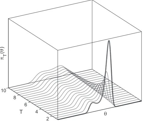
The issue of local trapping led to the development of the Simulated Annealing algorithm [14]. This involves the introduction of a factitious temperature2_{variableTsuch that, at high temperatures, the Markov chain is able to easily travel}

over local traps in the parameter space. The temperature variable is then reduced such that the fine details of the target distribution are gradually introduced – this is demonstrated graphically for a bimodal target PDF in Fig. 1(where

π

T represents one's target distribution at temperature T). The rate at which T is reduced is commonly referred to as the annealing schedule.

Although this does notguaranteethat the chain will converge on the optimum region of parameter space, Simulated Annealing has been established as a reliable optimisation algorithm. Soon after it was introduced several variants of Simulated Annealing were proposed[15,16]in which the spread of the proposal PDF is initially set to be large but then reduces with temperatureT(at a user-defined rate), thus encouraging the Markov chain to make large jumps at higher temperatures but conduct a more local search at lower temperatures.

When applied to Bayesian inference, the variableTcan be introduced such that it controls the influence of the likelihood on the posterior:

π

Tð

θ

ÞpPðDj

θ

;MÞTPð

θ

jMÞ: ð7Þ

Through using Eq.(7)as one's target distribution and defining an annealing schedule whereTvaries monotonically between 0 and 1, a gradual transition between the prior and posterior distribution can be realised. This concept was utilised in

[12,17,18]where, by exploiting this gradual transition from prior to posterior, MCMC algorithms were developed which can be used to sample from posterior parameter distributions with complex geometries (where multiple, or even a continuum of optimum parameter vectors exist).

The performance of any Simulated Annealing algorithm will be sensitive to the choice of annealing schedule – annealing too fast places one at risk of becoming stuck in a local trap (such that a long time is required for the Markov chain to converge to its stationary distribution) while annealing too slowly will prove to be computationally expensive. It is possible to overcome this issue through the use of‘adaptive’annealing schedules such as those proposed in[17–19].

While the afore-mentioned algorithms are undoubtedly powerful, they can prove to be computationally expensive. One of the main aims of the current paper is to present a relatively cheap annealing algorithm which, within the context of Bayesian inference, can be applied to computationally demanding models.

1.2. Model selection

The issue of model selection occurs when one must choose from a variety of competing model structures. This is complicated by the fact that models with more parameters will likely be able to better replicate some training data than models with less parameters. Consequently, if one judges models simply on their ability to replicate training data, then the most complex of the competing structures will always be accepted. Models which are overly complex for the problem at hand are referred to as overfitted. Such models are often poor representations of the physics involved in the system of interest and, as a result, are poorly suited to making future predictions.

For a scenario where different model structures are available, the probability that the modelMiis suitable given the data Dcan also be written using Bayes' theorem:

PðMij Þ ¼D

PðDjMiÞPðMiÞ

PðDÞ ð8Þ

thus allowing one to write therelativeprobability of two different models, given dataD, as

PðMijDÞ PðMjjDÞ

¼PðDjMiÞPðMiÞ PðDjMjÞPðMjÞ

ð9Þ

wherePðMiÞandPðMjÞrepresent one's prior beliefs in the suitability of each model (typically set equal to one another) and PðDjMÞis the evidence term in Eq.(1). It is possible to show that the Bayesian approach to model selection automatically prevents overfitting (see[8,20]for more information). However, as was described in the previous section, the evidence term is difficult to evaluate. As a result, one may instead choose to use a different model selection paradigm which is easier to evaluate than Eq.(9)but also retains the same model selection properties. In this work the Deviance Information Criterion (DIC)[21]is used as a model selection criterion.

Before describing the Deviance Information Criterion (DIC) it is convenient to first define the deviance:

Dð

_θ

Þ ¼ 2 lnPðDj

_θ

;MÞ ð10Þ

2

where, as stated previously,PðDj

_θ

;MÞis the likelihood. The expected DevianceE½Dð

_θ

Þis a measure of how well the model structureMfits the data (as the parameter vector has been marginalised). The DIC is then defined as

DIC¼2E½Dð

θ

ÞDð

θ

^Þ; ð11Þ

where

E½Dð

_θ

Þ ¼Z Pð

_θ

jD;MÞDð

_θ

Þd

θ

ð12Þ

and

^

θ

¼E½Pð

_θ

jD;MÞ ¼Z Pð

_θ

jD;MÞ

_θ

d

θ

ð13Þ

such that the ‘best’ estimate parametersð

_θ

^Þare defined as the expected value of the posterior parameter distribution. Essentially, the lower the DIC, the more favourable the model. It also has the desired property that it rewards model fidelity while penalising model complexity (see reference[22]for a more detailed discussion).

The DIC lends itself well to situations where one has sampled from the posterior parameter distribution using MCMC as, using the successive parameter vectors realised by the MCMC algorithmf

_θ

ð1Þ;

θ

ð2Þ

;…;

θ

ðMÞ

g, the optimum parameter vector

θ

^ can be approximated by

^

θ

1

M ∑ M

i¼1

θ

ðiÞ

ð14Þ

while the expected deviance can also be approximated by

E D

θ

1

M ∑ M

i¼1

D

θ

ðiÞ ð15Þ

thus allowing one to approximate the DIC. While this has been applied to synthetic data in [13], the current work demonstrates its application to real experimentally obtained data.

The paper is organised as follows. InSection 2the novel annealing algorithm is presented. InSection 3the experimental system of interest is described. In Section 4the results of the new annealing algorithm are analysed. This includes an analysis of the parameter correlations and predictive capabilities of competing model structures. The issue of model selection is then addressed using the Deviance Information Criterion (DIC).Section 5is concerned with presenting possible future work while the conclusions are presented inSection 6.

2. Data annealing

As stated in the previous section, MCMC methods can be used to generate samples from an unnormalised target PDF

π

ð

_θ

Þ. In the context of this paper the target PDF is given by

π

ð

_θ

Þ ¼PðDj

_θ

;MÞPð

_θ

jMÞ: ð16Þ

2 4 6 8 10

θ

T

π

T

(

θ

[image:4.544.157.395.57.258.2]

)

In practice it is usually desirable to evaluate the logarithm of the target PDF:

lnð

_π

ð

_θ

ÞÞ ¼lnðPðDj

_θ

;MÞÞþlnðPð

_θ

jMÞÞ ð17Þ

as, by first finding lna¼ln

π

ð

θ

0Þln

π

ð

θ

ðiÞÞ before evaluating a¼expðlnaÞ, one can often avoid numerical overflow/ underflow issues when calculatingEq. (4).

For the case where there areNmeasurements in the training data:

D¼ fD1;…;DNg ð18Þ

then, assuming that each measurement is mutually independent, the likelihood is given by

PðDj

θ

;MÞ ¼ ∏N

i¼1

PðDij

θ

;MÞ: ð19Þ

In the case investigated here the training data Dconsists of a vector of inputs fy1;y2;…;yNgand a vector of measured outputsfx1;x2;…;xNg(the physical meaning ofxandyis discussed inSection 3). Using a Gaussian error-prediction model allows the likelihood to be written as

PDj

θ

;M¼ ∏N

i¼1 1

ffiffiffiffiffiffi

2

π

p

σ

exp

1

2

σ

2ðxixi^ð

θ

Þ 2_Þ

ð20Þ

wherexi^ð

θ

Þrepresents the response of the model with parameters

θ

and

σ

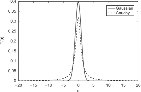
2is the likelihood variance (which can be treated as another parameter to be found). Consequently, a single evaluation of the likelihood requires the simulation ofNdata points. It is suggested here that, rather than usingTto control the influence of the likelihood on the posterior (as with Simulated Annealing), a similar effect can be achieved by varying the amount of data used in the likelihood. In other words, it is possible to increase the influence of the likelihood through the introduction of additional data points intoD. The rate at which the data points are introduced can be controlled according to a user-defined schedule–this is conceptually similar to the annealing schedule used in Simulated Annealing. The major advantage of this method is that it is computationally fast– in the early stages of the algorithm relatively few points need to be simulated by the model per evaluation of the likelihood. Throughout the current work this method is referred to as Data Annealing. It should be noted that the concept of annealing through the gradual addition of data points in the likelihood was proposed but not actually implemented in[12].

As was stated in Section 1, the Metropolis algorithm requires a user-defined proposal PDF to generate candidate parameter vectors

θ

0–this is often chosen to be a Gaussian. In the current work the proposal PDF will be denotedqð

_θ

0j

_θ

ðiÞÞ. In [15]it was suggested that, to reduce the probability of the Markov chain becoming stuck in a local trap, a proposal distribution with larger tails should be used in place of a Gaussian distribution. Specifically, it was suggested that a Cauchy distribution could be utilised as, while it is locally similar to a Gaussian, it possesses larger tails (as shown inFig. 2). This is desirable as, while the resulting Markov chain will spend the majority of the time conducting a local search of the parameter space, it will also occasionally propose relatively large jumps (thus increasing its ability to escape from local traps).

A disadvantage of this method becomes apparent when the dimension of the parameter space is greater than one as samples from the multidimensional Cauchy distribution are not uncorrelated–large jumps in one parameter will often be accompanied by large jumps in all of the other parameters[11]. In the author's opinion this seems rather restrictive. Here, it is proposed that each parameter in

θ

can be sampled independently from a one-dimensional Cauchy distribution such that, for parameter

θ

n:

q

θ

0nj

θ

ðiÞ n

¼

_πλ

n 1þ

θ

0 n

θ

ðiÞ n

λ

n

!2 0

@

1 A 2

4

3 5

1

ð21Þ

(where

λ

n controls the width of the distribution). Consequently, for the case where

θA

RND, the complete proposal

distribution is simply the product ofNDCauchy distributions:

qð

_θ

0j

_θ

ðiÞÞ ¼ ∏ND

n¼1 qð

_θ

0nj

θ

ðiÞ

nÞ: ð22Þ

3. Nonlinear system

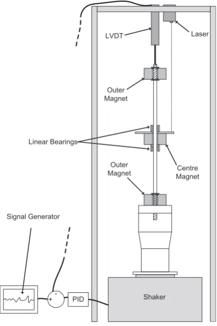
A schematic of the nonlinear dynamical system of interest is shown inFig. 3. A‘centre magnet’is positioned such that it is free to slide along an aluminium rod via a set of linear bearings. Two‘outer magnets’are attached to the aluminium rod– they are positioned such that their poles oppose that of the centre magnet (thus creating a magnetic restoring force on the centre magnet). Consequently, when excited by the shaker, the centre magnet experiences oscillatory motion relative to the shaker table. Originally developed in the context of nonlinear energy harvesting, it is known that the magnetic restoring force on the centre magnet can be closely approximated using a linear and cubic stiffness term (similar to the hardening spring Duffing oscillator)[23]. As a result, the equation of motion of the system is

m€x¼ c_zkzk3z3_{mgF; z¼xy ð23Þ}

wherexis the absolute displacement of the centre magnet,yis the displacement of the shaker table,mis the mass of the centre magnet,cis viscous damping,kis the linear stiffness,k3is the cubic stiffness andgis gravity. The training dataDis made up of discretely sampled values of the excitationy(measured using the LVDT inFig. 3) and of the centre magnet responsex(measured using the laser inFig. 3). The quantityFrepresents the force on the centre magnet as a result of friction effects. Three different friction models were considered. Firstly it was investigated whether the friction effects could be modelled simply using the viscous damping termc. Secondly, the Coulomb damping model was utilised such that

F¼Fcsgnðz_Þ ð24Þ

whereFcis a parameter to be estimated. Finally, it was hypothesised that the hyperbolic tangent model was appropriate:

F¼Fctanhð

_β

z_Þ ð25Þ

(where Fcand

β

are parameters to be estimated). Throughout this paper these candidate models are referred to as the

viscous, Coulomb and hyperbolic tangent models respectively. The hyperbolic tangent model has the property that

lim

β-1tanhð

β

z_Þ ¼sgnðz_Þ ð26Þ

such that it is able to form a close approximation to the signum function without being discontinuous atz_¼0. It should be noted that the mass of the centre magnet was measured accurately before testing and so, in the following analysis, it is not included in the vector of parameters to be estimated.

With regard to the applied excitation, a signal generator was used in conjunction with a PID controller to create a band-limited white noise acceleration. For a more detailed discussion of this experiment (which was also developed in the context of energy harvesting) the reader is directed towards references[24,25]. Two seconds of data measured at 1500 Hz was used as training data (this is shown inFig. 4).

4. Results

4.1. Markov chain Monte Carlo

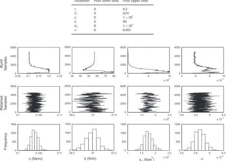
Uniform (but not improper) prior distributions were used in all runs of the Data Annealing algorithm. The upper and lower limits of the priors for each parameter are shown in Table 1. A uncorrelated Gaussian error-prediction model (as described inSection 2) was used in the likelihood. It was assumed that the standard deviation of the likelihood (

σ

) was constant throughout the experimental test. In each of the following cases the value of

σ

was estimated alongside the other model parameters.

−20 −15 −10 −5 0 5 10 15 20

0 0.05 0.1 0.15 0.2 0.25 0.3 0.35 0.4

θ

P(

θ

)

[image:6.544.154.395.58.215.2]

Gaussian Cauchy

For each model the Data Annealing algorithm was used to generate 50 000 samples of

θ

. The proposal distribution shown in Eq.(22)was used with

λ

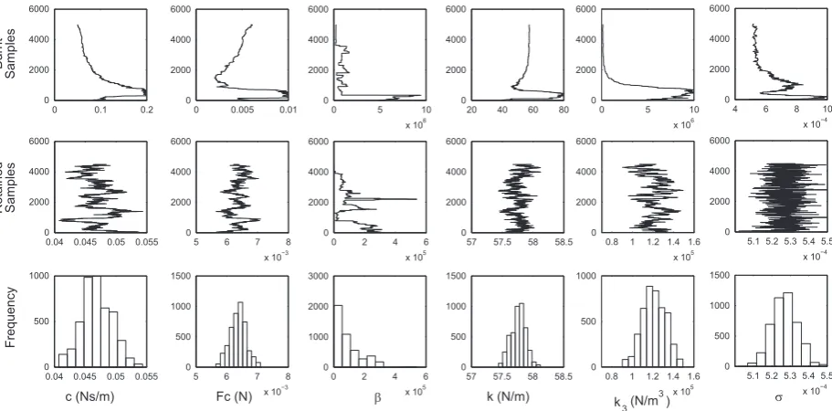
¼0:005 for each parameter. For the initial sample the dataDused in the likelihood consisted of 2 points (fy1;y2gandfx1;x2g). Additional data points were then introduced into the likelihood in a linear fashion for the first 2000 samples until the dataDcontained 3000 values of inputðyÞand 3000 values of the corresponding response (x). The amount of dataDwas then held constant for the remaining samples. The nonstationary portion of the resulting Markov chains were removed. To increase the independence between samples only every tenth sample from the resulting Markov chain was used to approximate the marginal PDFs of the posterior distribution.

The resulting Markov chains and parameter histograms for the viscous damping, Coulomb and hyperbolic tangent models are shown inFigs. 5,6and7respectively. As desired, use of the Data Annealing algorithm has allowed the Markov

Shaker +

-Signal Generator

PID

Laser LVDT

Linear Bearings

Centre Magnet Outer

[image:7.544.163.386.56.390.2]

Magnet Outer Magnet

Fig. 3.Schematic of experimental apparatus.

0 0.2 0.4 0.6 0.8 1 1.2 1.4 1.6 1.8 2 −6

−4 −2 0 2 4 6 x 10

−3

Time (s)

Absolute Displacement (m)

[image:7.544.145.396.430.576.2]

chain to make large jumps across the parameter space during the early stages while also allowing it to conduct a more local search once the chain has become stationary. To reiterate, this was achieved without having to vary the width of the proposal density.

With regard toFig. 7it should be noted that the Markov chain for the

β

parameter did not appear to become stationary. This demonstrates an interesting flaw in the MCMC algorithm used in this paper: it is not clear whether the non-stationarity of the Markov chain is a result of

β

being a nuisance parameter or of a poorly tuned MCMC algorithm. Upon closer inspection it became apparent that at no point did the chain transition into a region lower than

β

1000. Recalling that the hyperbolic tangent model forms a close approximation to the Coulomb model when a large value of

β

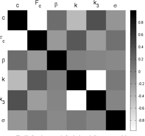
is utilised allows one to hypothesise that the Coulomb model may be more appropriate in this case (the ability of all the models to predict future response and the issues of model selection are discussed in the subsequent sections).

One of the advantages of using MCMC methods is that one can approximate the covariance matrix of the model parameters of a particular system. This is achieved by computing the correlation coefficients between the Markov chains of the different parameters. The resulting covariance matrices for the viscous, Coulomb and hyperbolic tangent models are shown inFigs. 8,9and10respectively. For all three models it is interesting to note that there appears to be a strong negative correlation between the linear stiffnesskand the nonlinear stiffness termk3. This is a relation which is possible to show using the technique of equivalent linearisation: the situation where one is attempting to model the response of a system with a nonlinear hardening spring as accurately as possible using an equivalent linear system. In such a case one must compensate for the lack of a nonlinear spring term via an increase in the linear spring term (see[26]for more details). In

Figs. 9and10it is also shown that there is a strong negative correlation between the viscous damping termcandFcwhich

[image:8.544.44.506.85.414.2]

controls the magnitude of friction in the system. This indicates that one may able to compensate for the lack of a friction model in a linear system through an increase in viscous damping. Again, this is something which can be shown using equivalent linearisation.

Table 1

Limits of uniform prior distribution.

Parameter Prior lower limit Prior upper limit

c 0 0.2

Fc 0 0.01

β 0 1107

k 0 80

k3 0 1107

σ 0 0.001

0.05 0.1 0.15 0.2 0.25 0 2000 4000 6000 Burnt Samples

0.1 0.105 0.11 0

2000 4000 6000

Retained Samples

0.1 0.105 0.11 0 500 1000 1500 Frequency c (Ns/m)

30 40 50 60 70 80 0

2000 4000 6000

56.5 57 57.5

0 2000 4000 6000

56.5 57 57.5

0 500 1000 1500

k (N/m)

0 5 10

x 10 0

2000 4000 6000

1 1.5 2 2.5

x 10 0

2000 4000 6000

1 1.5 2 2.5

x 10 0

500 1000 1500

k₃ (N/m3)

4 6 8 10

x 10 0

2000 4000 6000

5.6 5.8 6 6.2 x 10 0

2000 4000 6000

5.6 5.8 6 6.2 x 10 0 500 1000 1500 σ

4.2. Response predictions

Having obtained probabilistic estimates for the parameters, each model was used to predict the response of the system to 59 seconds of a new excitation (which was part of a different set of experimental data). This data set will be denotedDnewto distinguish it from the training dataD. As stated in[20], the Theorem of Total Probability can be used to obtain probabilistic estimates ofDnew:

PðDnewjD;MÞ ¼ Z

PðDnewjD;

θ

;MÞPð

θ

jD;MÞd

θ

ð27Þ

0 0.1 0.2

0 2000 4000 6000 Burnt Samples

0.04 0.05 0.06 0

2000 4000 6000

Retained Samples

0.04 0.05 0.06 0 500 1000 1500 Frequency c (Ns/m)

0 0.005 0.01 0

2000 4000 6000

5 6 7

x 10 0

2000 4000 6000

5 6 7

x 10 0

500 1000 1500

F_c (N)

20 40 60 80 0

2000 4000 6000

57.4 57.6 57.8 58 0

2000 4000 6000

57.4 57.6 57.8 58 0

500 1000 1500

k (N/m)

0 5 10

x 10 0

2000 4000 6000

0.8 1 1.2 1.4 1.6

x 10 0

2000 4000 6000

0.8 1 1.2 1.4 1.6

x 10 0

500 1000

k₃ (N/m3)

4 6 8 10

x 10 0

2000 4000 6000

5.2 5.4 5.6

x 10 0

2000 4000 6000

5.2 5.4 5.6

[image:9.544.39.508.55.287.2]

x 10 0 500 1000 1500 σ

Fig. 6. Results of the Data Annealing algorithm for the Coulomb model. The first row shows the burnt data during the annealing stage of the algorithm, the second row shows the thinned Markov chain with the burn period removed and the third row shows the resulting parameter histograms.

0 0.1 0.2 0 2000 4000 6000 Burnt Samples

0.04 0.045 0.05 0.055 0

2000 4000 6000

Retained Samples

0.04 0.045 0.05 0.055 0

500 1000

Frequency

c (Ns/m)

0 0.005 0.01 0

2000 4000 6000

5 6 7 8

x 10 0

2000 4000 6000

5 6 7 8

x 10 0 500 1000 1500 Fc (N)

0 5 10

x 10 0

2000 4000 6000

0 2 4 6

x 10 0

2000 4000 6000

0 2 4 6

x 10 0 1000 2000 3000 β

20 40 60 80 0

2000 4000 6000

57 57.5 58 58.5 0

2000 4000 6000

57 57.5 58 58.5 0

500 1000 1500

k (N/m)

0 5 10

x 10 0

2000 4000 6000

0.8 1 1.2 1.4 1.6 x 10 0

2000 4000 6000

0.8 1 1.2 1.4 1.6

x 10 0

500 1000

k₃ (N/m3)

4 6 8 10 x 10 0

2000 4000 6000

5.1 5.2 5.3 5.4 5.5

x 10 0

2000 4000 6000

5.1 5.2 5.3 5.4 5.5 x 10 0 500 1000 1500 σ

Fig. 7. Results of the Data Annealing algorithm for the hyperbolic tangent model. The first row shows the burnt data during the annealing stage of the

[image:9.544.44.500.338.563.2]

1

M ∑ M

i¼1

P Dnew

θ

ðiÞ

;M

ð28Þ

where

θ

ðiÞ_;i¼1_;…;M, are the posterior samples generated by the Data Annealing algorithm.

[image:10.544.156.402.57.287.2]

An alternative method was suggested in[13]where, to account for the assumption that the system parameters are time-independent, it was suggested that one could sample a new parameter vector from the posteriorafter every time step of the model simulation. In the current work, both methods of uncertainty propagation were investigated (using a total ensemble of 50 model predictions) although it was found that the results were indistinguishable.

[image:10.544.154.401.63.508.2]

Figs. 11 and 12show the ability of the viscous and Coulomb models to replicate one second of the experimentally obtained response (with confidence bounds). It can be seen that both models have replicated the response of the system to a good level of accuracy. The prediction made by the hyperbolic tangent model is not shown here as it was indistinguishable from that of the Coulomb model. This strengthens the hypothesis that the Coulomb damping model is preferable to the hyperbolic tangent model as it is able to generate a very similar response despite having less parameters.

Fig. 8.Covariance matrix for the viscous model.

[image:10.544.155.402.286.523.2]

The mean square error (MSE) between the predicted future response from each model and the measured experimental response was calculated. This was taken over the entire 59 seconds of data. The MCMC samples realised in the previous section were then used to calculate the Deviance Information Criterion. The results are shown inTable 2. The MSE for the Coulomb and hyperbolic tangent models is significantly lower than that for the viscous model while the MSE for the Coulomb and hyperbolic tangent models is identical. This indicates that while the inclusion of a friction model has enhanced performance, the hyperbolic tangent model is simply acting as an approximation for the Coulomb model. This is confirmed by the Deviance Information Criterion which indicates that the Coulomb model is the most appropriate (thus confirming what was already suspected). For the sake of completeness, the ability of the Coulomb model to replicate the full 59 seconds of experimental data is shown inFig. 13.

5. Discussion and future work

One of the disadvantages of Data Annealing is that, relative to algorithms such as Transitional MCMC (TMCMC)[17]and Asymptotically Independent Markov Sampling (AIMS)[18], the user has less control over the rate at which the influence of the likelihood is increased during the annealing process. This is because TMCMC and AIMS utilise the temperature variable in such a way that the transition from prior to posterior can be controlled in a continuous manner. The ability to select each temperature T from the set TA½0;1 (subject to the constraint that the sequence of temperature values must increase monotonically from 0 to 1) essentially means that the user has an uncountably infinite set of possible annealing schedules available to them. This flexibility is lost when utilising the Data Annealing algorithm as the transition from prior to posterior is influenced by the sensitivity of one's parameter estimates to the introduction of a new data set. As a topic of future work the author aims to develop a version of Data Annealing algorithm which allows the user to have greater control over the annealing schedule.

Throughout this paper the DIC was used as a model selection criterion. The disadvantage of this approach is that, although it can be estimated using samples from the posterior, it is an ad hoc penalty term which can only be used when each model has a single optimum parameter vector. A more complete approach would involve a variation of Data Annealing which was also able to estimate the model evidence (Eq.(2)) (thus allowing the relative plausibility of competing model structures to be investigated within a Bayesian framework). Consequently, for future work the author intends to investi-gate whether Data Annealing can be combined with other MCMC methods which are capable of estimating the model evidence–such methods could include Simulated Tempering[27,28], Reversible Jump MCMC[29], TMCMC[17], AIMS[18]

and Nested Sampling[30].

6. Conclusions

[image:11.544.150.393.57.285.2]

In this paper the system identification of an experimental nonlinear dynamical system was investigated using three competing model structures. A new MCMC algorithm named‘Data Annealing’was proposed. Being conceptually similar to Simulated Annealing, Data Annealing is designed such that, at its initial stages, the prior distribution dominates the shape of the target distribution. This allows the Markov chain to move freely around the parameter space. Additional training data is

then progressively introduced into the likelihood such that the influence of the likelihood on the posterior is gradually increased. This computationally cheap method improves the ability of the Markov chain to converge on the globally optimum region of the parameter space without getting stuck in‘local traps’. Additionally, the Data Annealing algorithm utilises a proposal distribution which allows it to conduct a local search of the parameter space accompanied by occasional long jumps. It was shown that this proposal distribution is well suited to the problem at hand as it initially allows the Markov chain to explore large regions of the parameter space while is also capable of providing a more local search once the chain has converged. This was achieved without having to alter the width of the proposal distribution. Having demonstrated the Data Annealing algorithm on a real system identification problem, the resulting Markov chains were used to extract approximate covariance matrices for all of the models investigated, thus revealing information about parameter correlations

10 10.1 10.2 10.3 10.4 10.5 10.6 10.7 10.8 10.9 11

−8 −6 −4 −2 0 2 4 6 8x 10

−3

Time (s)

Absolute Displacement (m)

[image:12.544.102.447.59.243.2]

Model Experiment ± 3 σ

Fig. 11.Comparison between one second of viscous model prediction (black) and one second of experimental data (grey) where dashed black lines

represent 3σconfidence bounds.

10 10.1 10.2 10.3 10.4 10.5 10.6 10.7 10.8 10.9 11

−8 −6 −4 −2 0 2 4 6 8x 10

−3

Time (s)

Absolute Displcement (m)

Model Experiment

[image:12.544.101.446.284.464.2]

± 3 σ

Fig. 12. Comparison between one second of Coulomb model prediction (black) and one second of experimental data (grey) where dashed black lines

represent 3σconfidence bounds.

Table 2

Mean square error between model and experiment and Deviance Information Criterion for the viscous, Coulomb and hyperbolic tangent models.

Model Parameter number MSE DIC

Viscous 3 0.0175 1.1047106

Coulomb 4 0.0085 1.1449106

[image:12.544.149.397.533.584.2]

induced by the data. Finally, a model selection criterion known as the Deviance Information Criterion was used to select the most appropriate model from the set of competing structures. It was shown that the DIC can be used to identify a model which can accurately replicate a set of training data without being overfitted (relative to the other elements in a set of user-defined model structures).

Acknowledgements

The author would like to thank James L. Beck from the California Institute of Technology for his talk at IMAC XXXI which inspired much of the work shown in this paper.

This work was conducted as part of an EPSRC fellowship and is also closely aligned to the EPSRC Programme Grant ‘Engineering Nonlinearity’EP/K003836/1.

References

[1]M.W. Vanik, J.L. Beck, S.-K. Au, Bayesian probabilistic approach to structural health monitoring, J. Eng. Mech. 126 (7) (2000) 738–745.

[2]K.-V. Yuen, L.S. Katafygiotis, Bayesian fast Fourier transform approach for modal updating using ambient data, Adv. Struct. Eng. 6 (2) (2003) 81–95. [3]J. Ching, J.L. Beck, K.A. Porter, Bayesian state and parameter estimation of uncertain dynamical systems, Probab. Eng. Mech. 21 (1) (2006) 81–96. [4]W. Becker, K. Worden, J. Rowson, Bayesian sensitivity analysis of bifurcating nonlinear models, Mech. Syst. Signal Process. 34 (1) (2013) 57–75. [5]S.-K. Au, Connecting Bayesian and frequentist quantification of parameter uncertainty in system identification, Mech. Syst. Signal Process. 29 (2012)

328–342.

[6]E. Simoen, C. Papadimitriou, G. Lombaert, On prediction error correlation in Bayesian model updating, J. Sound Vib. 332 (18) (2013) 4136–4152. [7]J.L. Beck, L.S. Katafygiotis, Updating models and their uncertainties. i: Bayesian statistical framework, J. Eng. Mech. 124 (4) (1998) 455–461. [8]D.J.C. MacKay, Information Theory, Inference and Learning Algorithms, Cambridge University Press, Cambridge, CB2 8RU, UK, 2003. [9]J.L. Doob, Stochastic Processes, Wiley Publications in Statistics, Wiley, Oxford, OX4 2DQ, UK, 1953.

[10]S. Cheung, J.L. Beck, Bayesian model updating using hybrid Monte Carlo simulation with application to structural dynamic models with many

uncertain parameters, J. Eng. Mech. 135 (4) (2009) 243–255.

[11] R.M. Neal, Probabilistic Inference using Markov Chain Monte Carlo Methods, Technical Report, University of Toronto, 1993.

[12]J.L. Beck, S.-K. Au, Bayesian updating of structural models and reliability using Markov chain Monte Carlo simulation, J. Eng. Mech. 128 (4) (2002) 380–391.

[13]K. Worden, J.J. Hensman, Parameter estimation and model selection for a class of hysteretic systems using Bayesian inference, Mech. Syst. Signal Process. 32 (2012) 153–169.

[14]S. Kirkpatrick, M.P. Vecchi, Optimization by simulated annealing, Science 220 (4598) (1983) 671–680. [15]H. Szu, R. Hartley, Fast simulated annealing, Phys. Lett. A 122 (3–4) (1987) 157–162.

[16]L. Ingber, Very fast simulated re-annealing, Math. Comput. Modell. 12 (8) (1989) 967–973.

[17] J. Ching, Y.C. Chen, Transitional Markov chain Monte Carlo method for Bayesian model updating, model class selection, and model averaging, J. Eng. Mech. 133 (7) (2007) 816–832.

[18]J.L. Beck, K.M. Zuev, Asymptotically independent Markov sampling: a new Markov chain Monte Carlo scheme for Bayesian inference, Int. J. Uncertain Quantif. 3 (5) (2013).

[19]P. Salamon, J.D. Nulton, J.R. Harland, J. Pedersen, G. Ruppeiner, L. Liao, Simulated annealing with constant thermodynamic speed, Comput. Phys.

Commun. 49 (3) (1988) 423–428.

[20] M. Muto, J.L. Beck, Bayesian updating and model class selection for hysteretic structural models using stochastic simulation, J. Vib. Control 14 (1–2) (2008) 7–34.

[21]D.J. Spiegelhalter, N.G. Best, B.P. Carlin, A. Van Der Linde, Bayesian measures of model complexity and fit, J. R. Stat. Soc.: Ser. B (Stat. Methodol.) 64 (4) (2002) 583–639.

[22] A. Gelman, J.B. Carlin, H.S. Stern, D.B. Rubin, Bayesian Data Analysis, Chapman & Hall, CRC, Boca Raton, Florida 33431, US, 2003. [23] B.P. Mann, N.D. Sims, Energy harvesting from the nonlinear oscillations of magnetic levitation, J. Sound Vib. 319 (1) (2009) 515–530.

[24] P.L. Green, K. Worden, K. Atallah, N.D. Sims, The effect of Duffing-type non-linearities and Coulomb damping on the response of an energy harvester to random excitations, J. Intell. Mater. Syst. Struct. 23 (18) (2012) 2039–2054.

[25] P.L. Green, K. Worden, K. Atallah, N.D. Sims, The benefits of Duffing-type nonlinearities and electrical optimisation of a mono-stable energy harvester under white Gaussian excitations, J. Sound Vib. 331 (20) (2012) 4504–4517.

0 5 10 15

−0.01 0 0.01

15 20 25 30

−0.01 0 0.01

30 35 40 45

−0.01 0 0.01

Absolute Displacement (m)

45 50 55 60

−0.01 0 0.01

Time (s)

Model Experiment

[image:13.544.105.437.58.198.2]

± 3 σ

Fig. 13. Comparison between 59 seconds of Coulomb model prediction (black) and 59 seconds of experimental data (grey) where dashed black lines

[26] K. Worden, G.R. Tomlinson, Nonlinearity in Structural Dynamics: Detection, Identification and Modelling, Taylor & Francis, Bristol, BS1 6BE, UK, 2010. [27]E. Marinari, G. Parisi, Simulated tempering: a new Monte Carlo scheme, EPL (Europhys. Lett.) 19 (6) (1992) 451.

[28] C.J. Geyer, E.A. Thompson, Annealing Markov chain Monte Carlo with applications to ancestral inference, J. Am. Stat. Assoc. 90 (431) (1995) 909–920.

[29] P.J. Green, Reversible jump Markov chain Monte Carlo computation and Bayesian model determination, Biometrika 82 (4) (1995) 711–732.