Article:
Halliday, David M orcid.org/0000-0001-9957-0983 (2015) Nonparametric directionality
measures for time series and point process data. Journal of integrative neuroscience. pp.
253-577. ISSN 0219-6352
https://doi.org/10.1142/S0219635215300127
[email protected] https://eprints.whiterose.ac.uk/
Reuse
["licenses_typename_other" not defined]
Takedown
If you consider content in White Rose Research Online to be in breach of UK law, please notify us by
Non-parametric directionality measures for time series and point process data.∗
David M. Halliday
Department of Electronics, University of York York, YO10 5DD, UK
The need to determine the directionality of interactions between neural signals is a key requirement for analysis of multichannel recordings. Approaches most commonly used are parametric, typically relying on autoregressive models. A number of concerns have been expressed regarding parametric approaches, thus there is a need to consider alternatives. We present an alternative non-parametric approach for construction of directionality mea-sures for bivariate random processes. The method combines time and frequency domain representations of bivariate data to decompose the correlation by direction. Our framework generates two sets of complementary measures, a set of scalar measures, which decompose the total product moment correlation coefficient summatively into three terms by direction and a set of functions which decompose the coherence summatively at each frequency into three terms by direction: forward direction, reverse direction and instantaneous interac-tion. It can be undertaken as an addition to a standard bivariate spectral and coherence analysis, and applied to either time series or point-process (spike train) data or mixtures of the two (hybrid data). In this article we demonstrate application to spike train data using simulated cortical neurone networks and application to experimental data from isolated muscle spindle sensory endings subject to random efferent stimulation.
Keywords: Directionality; Coherence; Non parametric; Time series; Point process; Net-works; Granger causality
1. Introduction
In many scientific fields there is a need to extract information from multivariate time-series or point-process data that can provide insight into the underlying dynamics of the system under study. The field of networks and network theory (Newman, 2010) has emerged in recent years as an approach that has broad applicability, where a graphical network (Whittaker, 1990) is used to represent the data, with individual time series or point processes as nodes in the network and the pattern of interac-tions as edges (or links) in the network. This approach has been applied to genetic regulatory networks (Karlebach and Shamir, 2008; Crespo et al., 2012) metabolic networks (Jeong et al., 2000), man made networks (Carvalho et al., 2009) and neu-ronal networks using neuroimaging (Rubinov and Sporns, 2010; Kaiser, 2011) and
∗Preprint 9 Oct 2014. Revised 25 Feb 2015
electrophysiological (Medkour et al., 2009) data sets. The field of network theory provides a range of tools to classify the network structure (Newman, 2010; Rubinov and Sporns, 2010), which takes as the starting point the adjacency matrix in binary form describing the pattern of interactions between the time-series or point-process data.
The first step in applying network theory is to establish the pattern of inter-actions between the nodes (time-series or point-processes). In application to multi-variate neural data, two classes of networks are used, these are directed and undi-rected networks, often referred to as functional and effective connectivity graphi-cal networks (Rubinov and Sporns, 2010). Undirected networks are typigraphi-cally based on measures of correlation between pairs of variables (Rubinov and Sporns, 2010; Kaiser, 2011) although partial correlation has also been used (Rosenberg et al., 1998; Salvador et al., 2005; Halliday, 2005; Medkour et al., 2009). The most commonly applied correlation measures are non-parametric using time and frequency domain measures of correlation (Medkour et al., 2009; Rosenberg et al., 1998, 1989)
Directed networks which measure the effective connectivity are concerned with cause-and-effect, i.e. establishing directionality or causal effects in the network (Ru-binov and Sporns, 2010). Approaches typically adopted here are parametric, these rely on a model to describe the underlying interactions. Granger (1969) introduced the concept of using residual variances to determine cause and effect in random processes, with application to economic time series, leading to the term “Granger causality”. A variation on this was developed by Geweke (1982, 1984) using a similar parametric approach to generate measures based on log ratios of residual variances. These studies use autoregressive models to describe the pattern of interactions be-tween the time-series. The Granger and Geweke measures and variants of these have been widely applied to describe directed interactions in neurophysiological data sets (Baccala et al., 2001; Kaminski et al., 2001; Chen et al., 2006; Schelter et al., 2006; Chicharro, 2012). Although parametric approaches are widely used, a number of studies have suggested reasons why parametric approaches may not be appropriate. Gersch (1972) showed examples of misclassification of interactions using paramet-ric as opposed to non parametparamet-ric measures. Thomson (1990) compared multi-taper spectral estimates with autoregressive estimates and found the former to be better suited to climate time series data. (Thomson and Chave, 1991) suggested that AR models are not well suited to capture the structure in time series routinely encoun-tered in scientific and engineering problems. It has also been noted that in some cases negative values can be obtained for parametric causality estimates (Geweke, 1982; Lindsay and Rosenberg, 2011).
in-troduced a frequency domain approach using a progression of spectra and partial spectra to infer network structure. These non-parametric approaches are not subject to the concerns regarding autoregressive models. However, as yet, non parametric approaches do not provide direct quantitative measures of directionality similar to those available from parametric approaches. This may explain in part the restricted applications of non-parametric directionality analyses. There have been few stud-ies of directionality applied to neuronal spike train (or point process) data, in part because of the inability to apply autoregressive models to point-process data. One approach has been suggested recently that uses a recursive factorisation of the spec-tral matrix (Wilson, 1972) and has been applied to generate Granger like measures (Dhamala et al., 2008a,b). It has been pointed out (Lindsay and Rosenberg, 2011) that the approach is partly parametric as it relies on a parametric model for the observations. Thus it could also be classified as a parametric approach and may be subject to some of the concerns regarding the validity of representation.
This paper introduces a framework for non-parametric directionality measures which quantify directed interactions between bivariate data. A combined time and frequency domain approach is used to decompose the coherence function by di-rection. In addition, scalar metrics are introduced which quantify the direction of interaction between the signals. The measures have a direct interpretation in terms of the overall strength of correlation. We use the term directionality in preference to causality, although the motivation is similar. A particular strength of the proposed approach is applicability to both time series and point process data.
Section 2 describes method including practical aspects related to estimation and the setting of confidence limits. Section 3 illustrates application of our non-parametric approach to neuronal spike train data using simulated cortical neurone interactions and application to single unit data from identified single muscle spindle sensory endings subject to efferent stimulation. Section 4 discusses the results and considers a number of issues related to the broader applicability of the approach and how our metrics relate to those obtained from parametric approaches.
2. Methods
2.1. The coherence function and R2 measure
The coherence between two random processes (x, y) is defined as (Brillinger, 1975; Priestley, 1981; Rosenberg et al., 1989)
|Ryx(ω)|2 = |
fyx(ω)|2
fxx(ω)fyy(ω)
(2.1)
wherefyx(ω) is the cross power spectral density (or cross-spectrum) between xand
y, and fyx(ω) andfyx(ω) are the auto spectra at frequency ω.
The total product moment correlation between (x, y), which we denote as Ryx2 , can be recovered by integration of the coherence (Pierce, 1979)
Ryx2 = 1 2π
∫ +π
−π |
Ryx(ω)|2dω (2.2)
The coherence in (2.2) is defined over the normalised angular frequency range [−π,+π]. Pierce (1979) uses this definition to obtain the squared correlation coef-ficient,R2, by integrating coherence whenx is the input to and y the output from
a linear regression model. Equation (2.2) allows the R2 measure to be calculated
by integrating over frequencies and establishes an important reference point for our framework. The decomposition ofR2
yxby direction is achieved using a novel form of
filtering which reduces the coherence to the cross spectrum.
2.2. MMSE whitening - reducing coherence to the cross spectrum
The coherence, (2.1) is defined as a ratio. Pierce (1979) notes that if the autospectra are assumed white then coherence reduces to the cross-spectrum. However, in gen-eral, spike trains and time series will not have white PSD estimates. The method of pre-whitening (Press and Tukey, 1956) can be used, where a signal is filtered prior to spectral analysis to bring its spectral content closer to that of white noise. A common approach to pre-whitening is to create a residual series after fitting a low order AR model to each processxandy(Percival and Walden, 1993). Pre-whitening can be advantageous in reducing undesirable aspects such as spectral leakage (Per-cival and Walden, 1993), but in the majority of cases the target of achieving a white sequence prior to spectral analysis is only met approximately, this does not allow replacement of the magnitude squared coherence by the magnitude squared cross-spectrum without degradation of the reliability of the coherence estimate.
We adopt the optimal whitening or minimum mean square error (MMSE) whiten-ing scheme introduced by Eldar and Oppenheim (2003). The Optimal whitenwhiten-ing filter for a zero-mean stationary random process, x, with PSD fxx(ω) is given by
(Eldar and Oppenheim, 2003, Theorem 3).
wxx(ω) =σfxx(ω)−1/2 (2.3)
whereσ is a fixed constant, σ >0. Denoting the whitened spectrum asfw
xx(ω), the
MMSE whitening procedure generates a whitened spectrum: fw
case we wish σ2 = 1, thus σ= 1 in equation (2.3). The pre-whitening filter defined in equation (2.3) is a non-causal zero phase phase filter with magnitude proportional to the inverse square root of the PSD fxx(ω).
This procedure is equivalent to generating two new (or derived) random pro-cesses, xw andyw, which have spectra equal to 1 at all frequencies
fxxw(ω) = 1, fyyw(ω) = 1 (2.4)
The cross spectrum between the two whitened sequences is fyxw(ω), and a co-herence estimate calculated using equation (2.1), in conjunction with equation (2.4) gives
Rwyx(ω)
2
= fyxw(ω)
2
(2.5)
Our framework is applicable to both time series and point process signals. The MMSE filtering step derives processes with spectra equal to 1 at all frequencies. Following this whitening/filtering step point process signals can no longer be con-sidered as spike trains. In the context of the present analysis the output of the MMSE whitening procedure for spike trains will be a continuous process which has a constant spectrum. The MMSE whitening step for time series similarly derives a continuous process with a constant spectrum. The two derived continuous processes have the same correlation structure as the original bivariate spike train or time se-ries data. Brillinger (1974) notes that a common frequency domain approach can be applied to time series and point process signals, where parameter estimates having the same statistical results can be constructed in the same manner after evaluation of the relevant Fourier transforms.
The filtering step to derive the whitened processes xw and yw uses two separate
univariate filters in the MMSE framework as opposed to a single optimal whitening transformation derived from the inverse square root of the covariance matrix (Eldar and Oppenheim, 2003). A single transformation would effectively orthogonalize the two random processes removing both within-variable and between-variable effects, and would not provide a useful approach to estimating directionality. The effect of the two pre-whitening filters is to remove any structure in the auto-correlation of the original sequencesx andy. The relationship between the variables is preserved, coherence is insensitive to linear transformations of the original signals (Priestley, 1981). Thus the two coherence functions in equations (2.1) and (2.5) are equivalent
Rwyx(ω)
2
=|Ryx(ω)|2 (2.6)
The coherence between the whitened processes, |Rw
yx(ω)|2 =|fyxw(ω)|2, has no terms
in the denominator and can thus be decomposed to obtain directionality measures.
2.3. Directionality measures - time domain The scalar measure of dependence between x andy,R2
yx, can now be written as
R2yx= 1 2π
∫ +π
−π
fyxw(ω)
2
To decomposeR2yx by direction we define a correlation measure in the time domain,
ρyx(τ), with time lagτ, which forms a Fourier transform pair with the pre-whitened
cross spectrum,fyxw(ω), as
ρyx(τ) =
1 2π
∫ +π
−π
fyxw(ω)eiωτdω (2.8)
The definitions in equations (2.7 - 2.8)assume second order spectra are periodic in
ω with period 2π (Brillinger, 1975, Th 2.5.1). ThenR2yx can be decomposed by lag according to
R2yx=
∫ +∞
−∞ |
ρyx(τ)|2dτ (2.9)
Equation (2.9) can be proved using Parseval’s theorem (e.g. Priestley, 1981, Ch 4) Further decomposition of R2yx by lag to obtain measures of directionality is achieved by selecting the required lag range in equation (2.9). We define and use three measures which from a subset ofR2yx. These areR2yx;−,R2yx;0 andRyx;+2 which measure the directionality: x ← y, x ↔ y and x → y, respectively. Thus R2
yx is
decomposed summatively into three components:
R2yx=
∫
τ <0|
ρyx(τ)|2dτ +|ρyx(0)|2+
∫
τ >0|
ρyx(τ)|2dτ (2.10)
This can be written using our extended notation as
R2yx=R2yx;−+R2yx;0+R2yx;+ (2.11) The termR2
yx;− quantifies the contribution from future xt to the presentyt, using
values with negative lags fromρyx(τ). The term,Ryx;02 has a single component that
quantifies the contribution of the instantaneous interaction between xt and yt to
R2yx, using the single valueρyx(0). The termR2yx;+ quantifies the contribution from
pastxt to the presentyt, using values with positive lags from ρyx(τ).
2.4. Directionality measures in the frequency domain
In this section we consider how the directionality measures,R2yx;−,R2yx;0 andR2yx;+
can be decomposed as a function of frequency. To do this we define two sets of corresponding measures: fyx;′ −(ω), fyx;0′ (ω), fyx;+′ (ω) and |R′yx;−(ω)|2, |Ryx;0′ (ω)|2, |R′yx;+(ω)|2. The first set of measures are defined by applying a Fourier transform to the functionρyx(τ) with different integration ranges forτ:
fyx;′ −(ω) =
∫
τ <0
ρyx(τ)e−iωτdτ (2.12)
fyx;0′ (ω) =ρyx(0) (2.13)
fyx;+′ (ω) =
∫
τ >0
The lag ranges used for τ here are the same as in equation (2.10), thusfyx;′ −(ω) is calculated using only negative lags fromρyx(τ) andfyx;+′ (ω) is calculated using only
positive lags from ρyx(τ). The measurefyx;0′ (ω) is constant over all frequencies, this
is just the Fourier transform of a scaled impulse atτ = 0 inρyx(τ). The originalR2yx
measure can be recovered from these by integrating over the full frequency range as, c.f. equation (2.2)
Ryx2 = 1 2π
(∫ +π
−π |
fyx;′ −(ω)|2dω +
∫ +π
−π |
fyx;0′ (ω)|2dω+
∫ +π
−π |
fyx;+′ (ω)|2dω )
(2.15)
This result is derived following the same arguments as for the proof of equation (2.9). The three directional measures can also be defined in terms of the f′ functions, for example
R2yx;− = 1 2π
∫ +π
−π |
fyx;′ −(ω)|2dω (2.16)
The equality in equations (2.15), (2.16) is valid when thef′ measures are integrated over the complete frequency range, [−π,+π]. Using the magnitude squared of each measure, |f′
yx;·(ω)|2, as an indication of the strength of the interaction at each fre-quency may not preserve the original variance bound (Priestley, 1981), as the sum of the three terms at each frequency may exceed the original coherence, |Ryx(ω)|2.
To overcome this we define a second set of measures, |R′
yx;−(ω)|2, |R′yx;0(ω)|2, |Ryx;+′ (ω)|2. These preserve the variance bound given by the original coherence es-timate at each frequency
|Ryx(ω)|2 =|R′yx;−(ω)|2+|Ryx;0′ (ω)|2+|R′yx;+(ω)|2 (2.17)
This is achieved by rescaling the original coherence according to the relative mag-nitude of the |fyx;′ ·(ω)|2 measures at each frequency
|R′yx;−(ω)|2 = |f ′
yx;−(ω)|2 |fyx;′ −(ω)|2+|f′
yx;0(ω)|2+|fyx;+′ (ω)|2 |
Ryx(ω)|2 (2.18)
|R′yx;0(ω)|2 = |f ′
yx;0(ω)|2 |fyx;′ −(ω)|2+|f′
yx;0(ω)|2+|fyx;+′ (ω)|2 |
Ryx(ω)|2 (2.19)
|R′yx;+(ω)|2 = |f ′
yx;+(ω)|2 |f′
yx;−(ω)|2+|fyx;0′ (ω)|2+|fyx;+′ (ω)|2 |
Ryx(ω)|2 (2.20)
The assumption underlying this re-scaling is that the|fyx;′ ·(ω)|2provide an indication of the relative strength of the directionality at each frequency (Pierce, 1979). To distinguish the two sets of measures from conventional cross-spectral densities and conventional coherence functions we use the notation f′ andR′.
2.5. R2
yx measures over a restricted frequency range
A further useful refinement is consideration of R2
yx calculated over a restricted
signals of interest is restricted to a particular frequency range. For example many neurophysiological signals are low pass in nature with little power and dependency above a specific cut-off frequency. If the Nyquist frequency is considerably higher than this cut-off frequency then calculation of R2
yx using equation 2.2 will include
values where the coherence is not significant. In such cases it may be appropriate to introduce an upper limit in the integration to calculateR2
yx;α as
R2yx;α= 1 2απ
∫ +απ
−απ |
Ryx(ω)|2dω (2.21)
whereαis a fractional multiplier for the nyquist frequency, 0< α≤1. To distinguish such measures they will be referred to asRyx;α2 and in the directional case asR2yx;−,α,
R2yx;0,α and R2yx;+,α. To calculate the directionality measures over a restricted fre-quency range we use theR′ measures, as these satisfy the residual variance bound, see equation (2.17). Thus
R2yx;−,α= 1 2π
∫ +απ
−απ |
R′yx;−(ω)|2dω (2.22)
A similar definition is used forR2
yx;0,αandR2yx;+,α. The numerical value ofαmay be
more usefully indicated as absolute frequency in Hz,f α. So the directional measures are then R2
yx;−,f α, Ryx;0,f α2 and Ryx;+,f α2 , where f α = αfN and fN is the nyquist
frequency, usually specified in Hz. This is the approach we adopt, thus R2yx;+,100
represents the directionality measurex→y at frequencies up to 100Hz.
Some caution is needed in selecting the value ofαparticularly if comparisons are made betweenR2
yx;α for different bivariate data which do not use the same value of
α. The choice of suitable values ofα are discussed in the results section.
2.6. Estimation and algorithmic details
This section gathers in one place all the necessary expressions to estimate our non parametric measures. The first step in the bivariate directionality analysis of two random processes xand y is to construct the auto- and cross-spectral estimates. A range of approaches exist for calculation of spectral densities, here we will adopt the approach of (Halliday et al., 1995) in which a record of duration R points is split intoL disjoint sections of lengthT points, withR=LT. To distinguish between a parameter and its estimate we will use a hat symbol,ˆ, to indicate an estimate, thus
ˆ
fxx(ω), ˆfyy(ω) and ˆfyx(ω) are the estimated auto- and cross-spectra constructed
using average periodograms, see Halliday et al. (1995, eq 5.2)
The pre-whitening filter for each process is estimated from equation (2.3) as
ˆ
wxx(ω) = ˆfxx(ω)−1/2 (2.23)
ˆ
wyy(ω) = ˆfyy(ω)−1/2 (2.24)
in a different pre-whitening filter for each process. From our perspective this is fine, the objective is to pre-whiten auto-spectral estimates to be identical to 1 at each frequency. The simplest approach to apply the filter is in the frequency domain by multiplying each discrete Fourier transform by the appropriate filter to get the whitened discrete Fourier transform for each segment, l
dwTx(ω, l) =dTx(ω, l) ˆwxx(ω) (l= 1, . . . L) (2.25)
dwTy(ω, l) =dTy(ω, l) ˆwyy(ω) (l= 1, . . . L) (2.26)
The whitened auto- and cross-spectral estimates, ˆfxxw(ω), ˆfyyw(ω) and ˆfyxw(ω), are then constructed using the same algorithmic approach as previously (average pe-riodograms in our case). The auto spectral estimates, ˆfxxw(ω) and ˆfyyw(ω), will now be 1 at all frequencies. Thus the coherence from the whitened sequences can be estimated as
|Rˆwyx(ω)|2=|fˆyxw(ω)|2 (2.27) This will be identical to the original coherence estimate before whitening,|Rˆyx(ω)|2,
the advantage now is that the pre-whitening process equates the magnitude squared coherence to the magnitude cross spectrum, allowing the directionality measures to be derived from the cross spectrum estimate, ˆfyxw(ω). The correlation,ρyx(τ), is
estimated using a standard inverse Fourier transform of length T (e.g. Halliday et al., 1995).
The overallR2
yx measure can be estimated in either the frequency domain from
equation (2.7) or in the time domain from equation (2.9).
ˆ
R2yx= 1
T ∑
j
|fˆyxw(ωj)|2 (2.28)
ˆ
R2yx=∑
k
ˆ
ρyx(τk)2 (2.29)
Here ωj are the discrete Fourier frequencies,ωj = 2πj/T. Both summations have T
terms. We do not distinguish between the two estimates in equations (2.28-2.29). In practice either can be used to estimate R2
yx, they give equivalent values.
The directionality measures can be calculated using ˆρyx(τ) as
ˆ
R2yx;−=∑
τ <0
ˆ
ρyx(τ)2 (2.30)
ˆ
R2yx;0= ˆρyx(0)2 (2.31)
ˆ
R2yx;+ =∑
τ >0
ˆ
ρyx(τ)2 (2.32)
where τ is lag specified as an integer in the range −T2 ≤τ < T2.
The frequency domain directionality measures use the quantitiesf′ in equations 2.12-2.14, and R′ in equations 2.18-2.20. The first of these are estimated as
ˆ
fyx;′ −(ωj) =
∑
τ <0
ˆ
fyx;0′ (ωj) = ˆρyx(0) (2.34)
ˆ
fyx;+′ (ωj) =
∑
τ >0
ρyx(τk)eiωjτ (2.35)
whereωj = 2πj/T. The quantities in equations 2.33-2.35 can be calculated using an
FFT algorithm of length T containing the relevant subset of ˆρyx(τ), padded with
zeros as appropriate. The R′ measures can be estimated directly by direct substi-tution of |fˆyx;′ ·(ωj)|2 estimates and coherence estimates, |Rˆyx(ω)|2, into equations
2.18-2.20, providing the estimates|Rˆ′yx;−(ω)|2,|Rˆyx;0′ (ω)|2 and |Rˆ′yx;+(ω)|2.
Calculation of the R2 scalar metrics over a limited frequency range needs the additional parameter α to be specified, where 0 < α ≤ 1. From equation 2.21 we can estimateR2yx;α as
ˆ
R2yx;α= 1
αT ∑
|j|<αT /2
|Rˆyx(ωj)|2 (2.36)
An estimate ofR2yx;−,α, equation 2.22, is ˆ
R2yx;−,α= 1
αT ∑
|j|<αT /2
|Rˆyx;′ −(ωj)|2 (2.37)
Similar expressions are used to estimate R2yx;0,α andR2yx;+,α.
2.7. Assessing significance in parameter estimates
Approaches for assessing the significance of features in autospectral estimates are described in Diggle (1990); Bokil et al. (2007). The metric R2yx can be viewed as a correlation coefficient between the bivariate random processes (x, y). Statistical aspects of the correlation coefficient are discussed in (Kendall and Stuart, 1961) where expressions for standard errors and setting of confidence limits are discussed for a range of scenarios including the case of no correlation. These expressions are based on calculation of a scalar product-moment correlation coefficient, calculated as a ratio of the covariance to the product of the standard deviations. In our case the correlation coefficientR2
yxis estimated by integrating across the coherence function,
thus the statistical distribution will be different. In the case of no correlation,R2yx= 0, the distribution of ˆR2
yx will tend to normal as it is based on a sum overT points,
see equation 2.28. Since ˆR2yx is derived from the estimated coherence, |Rˆyx(ω)|2,
we can use existing approaches to determine significance in coherence estimates to determine the significance of ˆR2yx. Significance levels for coherence estimates, based on a NULL hypothesis of uncorrelated data are discussed in Brillinger (1975); Rosenberg et al. (1989). In particular Rosenberg et al. (1989) provides an expression for the approximate upper 95% confidence limit for|Rˆyx(ω)|2 estimated through an
average periodogram overLdisjoint sections as
Our approach is to use this for ˆR2yx also: If the estimated coherence is significant at frequencies of interest then ˆR2yx can be interpreted as also significant at these frequencies. This assumes that estimation of ˆR2
yx over a reduced frequency range,
ˆ
R2yx;α, equation 2.36, incorporates the frequencies of interest. Equation 2.38 provides an approximate confidence limit based on the assumption of uncorrelated processes. A more detailed analysis can be found in Brillinger (1975) where it is shown that the covariance structure for different frequencies has terms of order O(
T−2)
. Concerns regarding the spread of correlation to adjacent frequencies can be addressed through using a longer segment length, T, at the expense of fewer segments, L.
The primary use of the functionρyx(τ) is to allow decomposition ofR2yxinto the
three components in equation (2.11). However, the measure may be useful visually as an indicator of the general characteristics of the interactions between random processes x andy. A graphical representation is likely to be the most useful way to present this, in which case the large sample behaviour needs to be investigated, and in particular confidence intervals derived. From the definition of ρyx(τ) in equation
(2.8) and the results in Halliday et al. (1995), Rigas (1983, Th 4.9.1), under the assumption of no correlation between processes x and y we can write
var{ρyx(τ)} ≈
(
1 2π
)2(
2π R
) ∫ π
−π
fxxw(ω)fyyw(ω)dω (2.39)
Here R is the record length or number of data points, R = LT. As a consequence of the MMSE pre-whitening step then fxxw(ω) =fyyw(ω) = 1, allω. Thus
var{ρ(τ)} ≈
(
1 2π
)2(
2π R
)
2π= 1
R (2.40)
The expected value and upper and lower 95% confidence limits can then be set as
0±1√.96
R (2.41)
Inclusion of horizontal lines at these values on plots of estimates ofρyx(τ) will provide
a useful guide to interpret the significance or otherwise of specific features at indi-vidual lags. Equation (2.41) provides approximate confidence limits that are based on the assumption of uncorrelated processes, where second and fourth order cross spectral terms are assumed zero, with additional terms of order O(
R−2log e(R))
(Rigas, 1983). A similar approach has proved useful for setting confidence limits on cross-covariance (cumulant density) estimates (Halliday et al., 1995).
Equation 2.41 can be used to assess significance of the scalar measures R2yx;−,
R2yx;0 andR2yx;+ which are estimated from ˆρyx(τ) using equations 2.30-2.32.
There-fore significant values of ˆρyx(τ) at lags τ <0 can be interpreted as an indication of
significant R2yx;−, and significant values of ˆρyx(τ) at lags τ > 0 can be interpreted
as an indication of significant R2yx;+. Similarly, a significant value of ˆρyx(0) can be
3. Results
3.1. Simulated 3 neurone networks
The data in this section was generated using simulated 3 neurone networks of cortical neurones with dynamcis similar to those in Halliday (2005). Each neuron was modelled using a biophysical point neurone conductance model (Rm = 40MΩ,
Cm = 0.5pF, τm = 20 ms) with resting potential, Vr = −74mV, firing threshold,
Vthresh = −54mV and partial reset threshold of Vreset = −60mV. The partial
re-set mechanism allows point cortical neurone models to mimic the firing variability seen in vivo (Troyer and Miller, 1997). Each neurone received large scale back-ground synaptic activation consisting of 100 excitatory inputs firing randomly at 40 spikes/sec (VEP SP = 300µV from rest,VEP SP = 220µV at Vthresh,τEP SP = 0.2ms,
reversal potential EEP SP = 0mV) and 25 inhibitory inputs firing randomly at 40
spikes/sec (VIP SP = 16µV atVthresh,τIP SP = 10ms, EIP SP =−74mV). This
back-ground activation generated membrane potential fluctuations with a mean value of -55mV and SD of 1.25mV (measured with threshold mechanism suppressed) thus simulating the balanced large scale input that cortical neurones typically receivein vivo (Destexhe et al., 2003).
The three neurone networks were connected in a range of configurations using both excitatory (VEP SP = 2000µV from rest,VEP SP = 2750µV atVthresh,τEP SP =
1ms, EEP SP = 0mV) and inhibitory connections (VIP SP = 1000µV at Vthresh,
τIP SP = 10ms,EIP SP =−74mV) as illustrated in figure 1. Each configuration was
run 10 times generating 100 seconds of spike train data for each run. The firing rates ranged from 8–21 spikes/sec and the coefficient of variation (COV) ranged from 0.70–0.95 across all runs. Spike timings for each neurone were saved using a sampling interval of ∆t= 1 ms.
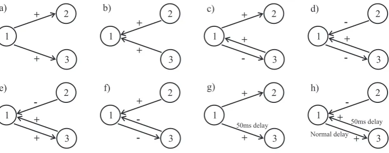
[image:13.595.113.504.546.700.2]1 3 2 1 3 2 + + + + a) b) 1 3 2 1 3 2 + -+ -+ c) d) 1 3 2 + -1 3 2 -+ + e) f) 50ms delay 1 3 2 -+ + h) 50ms delay Normal delay 1 3 2 + + g)
The results for the simulated data are illustrated in Figures 2-4 and Table 1. The examples in the figures use single data sets of 100 seconds duration each, the data in the table are mean values over 10 repeat runs of 100 secs duration each. Each run was analysed using the directionality analysis with a segment length of T = 1024 over L = 97 segments. All estimates in Figures 2-4 have been constructed using
L= 97 segments. In our average periodogram estimates the number of segments,L, is used to determine confidence limits, and it can also provide an indication of the sensitivity of the approach.
Coherence estimates are plotted as a function of frequency in cycles/sec,λj with
λj = j/(T∆t), 1 ≤ j ≤ T /2, where T is the segment length and ∆t the sampling
interval. Here ∆t= 10−3sec. The original coherence estimates,|Rˆ21(λj)|2 (Figure 2,
black lines) and |Rˆ31(λj)|2 (Figure 3, black lines) indicate there is significant
cor-relation between all spike train pairs, with significant coherence up to ∼150Hz for excitatory connections and up to ∼10 Hz for inhibitory connections. The quanti-tative directionality measures are in Table 1, an upper limit of 250 Hz was used to calculate the directionality measures (α = 0.5, f α = 250Hz, against a Nyquist frequency offN = 500Hz). The table shows the values for the estimated strength of
interactions between neurones 1→2, ˆR2
21;250 and between neurones 1→3, ˆR231;250,
as well as the estimated directional interactions: ˆR21;+,2502 and ˆR221;−,250for neurones 1 and 2, and ˆR231;+,250and ˆR231;−,250for neurones 1 and 3. In our notation, ˆR2yx repre-sents an estimate of the strength of interaction betweenx andyassuming processx
[image:14.595.114.455.600.717.2]is the input andyis the output. Thus the directional measures in table 1 all assume that neurone 1 is the reference (or input) neurone.
Table 1. Estimated values ofR221andR231at frequencies up to 250 Hz,f α= 250Hz, for the 3 neurone networks illustrated in figure 1, ˆR221;250, ˆR231;250, along with the estimated directional coupling strengths at frequencies up to 250 Hz, ˆR221;+,250,
ˆ
R221;−,250, ˆR231;+,250, ˆR231;−,250. The numbers in brackets for the directional measures are the percentage of the overall correlation in each direction. All values represent the mean over 10 repeat runs, where each run generated 100 seconds of spike train data for analysis.
Config. Rˆ221;250 Rˆ221;+,250 Rˆ221;−,250 Rˆ231;250 Rˆ231;+,250 Rˆ231;−,250
a 0.0712 0.0664 (93) 0.0046 (7) 0.0688 0.0638 (93) 0.0049 (7) b 0.0561 0.0045 (8) 0.0514 (92) 0.0600 0.0048 (8) 0.0551 (92) c 0.0802 0.0756 (94) 0.0045 (6) 0.0642 0.0059 (9) 0.0582 (91) d 0.0122 0.0050 (41) 0.0071 (58) 0.0641 0.0060 (9) 0.0580 (90) e 0.0124 0.0050 (40) 0.0074 (60) 0.0845 0.0364 (43) 0.0479 (57) f 0.0689 0.0046 (7) 0.0642 (93) 0.0139 0.0075 (54) 0.0064 (46) g 0.0722 0.0674 (93) 0.0046 (6) 0.0675 0.0629 (93) 0.0046 (7) h 0.0129 0.0053 (41) 0.0077 (59) 0.1225 0.0657 (54) 0.0568 (46)
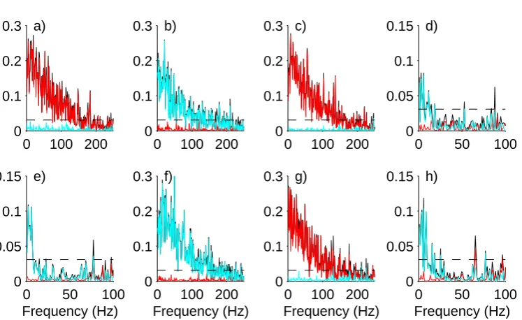
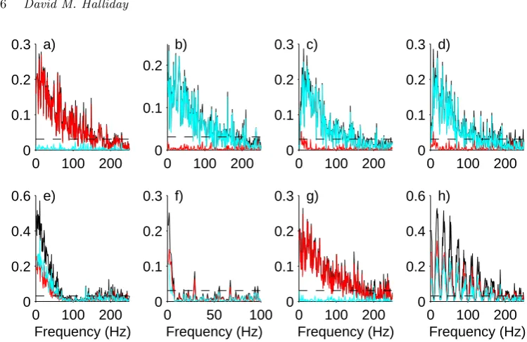
ˆ
R231;+,250, assign 93% of the overall correlation to the directions 1→2 and 1→3, in agreement with the configuration in figure 1a. In figure 2a, the decomposition of the coherence by direction shows|Rˆ′21;+(λj)|2 (red line) is almost identical to the
origi-nal coherence estimate (black line), whereas|Rˆ′
21;−(λj)|2 (blue line) is close to zero
at all frequencies. A similar interpretation applies to|Rˆ′31;+(λj)|2 and |Rˆ′31;−(λj)|2
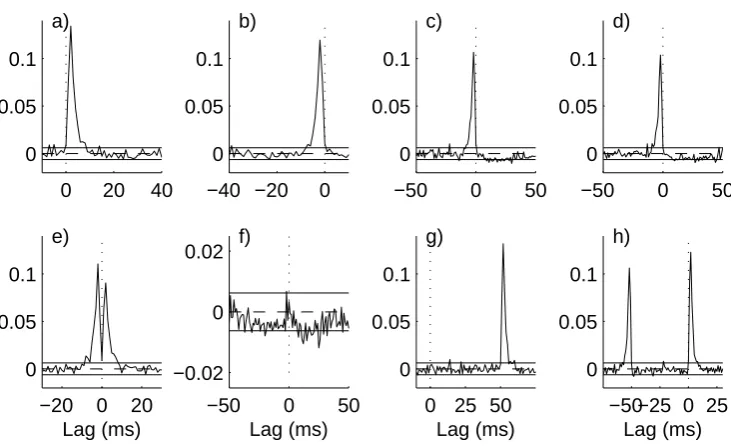
in figure 3a. The time domain estimate in figure 4a, ˆρ31(τ) has a significant peak
at positive latencies (maximum at +2 ms) and no significant features at negative latencies, in agreement with the configuration in figure 1a.
In configuration b), the directionality is reversed (fig 1b), this is correctly identi-fied by the entries in Table 1 (row 2), by the decomposition of coherence by direction (figs 2b, 3b) and by the decomposition in the time domain (fig 4b), where the sig-nificant features are at negative latencies.
Configurations c) and d) include reciprocal excitatory-inhibitory connections be-tween neurones 1 and 3. Figures 3c,d indicate that the excitatory connection is much stronger than the inhibitory connection. This is further illustrated in fig 4c,d where the relative timescales of the excitatory and inhibitory connections are highlighted -a short dur-ation pe-ak -at neg-ative l-atencies for excit-atory connection (time const-ant
τEP SP = 1ms) from 1←3 and a much broader depression only just reaching
signif-icance at positive latencies for inhibitory connection (τIP SP = 10ms) from 1 → 3.
Configurations e) and f) have symmetrical reciprocal connections between neurones 1 and 3. The metrics in table 1 assign around 50% of the overall correlation to each direction as expected. The symmetry is further highlight by the decomposition of the coherence in figs 3e, f and the decomposition by lag in figs 4e, f.
The final two configurations g) and h) are similar to a) and e), respectively, except there is an additional synaptic delay of 50 ms in the connection from 1→3 in a) and 1←3 in e). These two configurations demonstrate that the directionality metrics are not affected by the presence of additional delays in the pathways. For configuration g) the estimate in figure 3g is not distinguishable from that in figure 3a. The delay is clearly seen in figure 4g. The directional metrics in Table 1 row g are identical to those in row a. In configuration h) the coupled neurones now oscillate with a fundamental frequency around 18 Hz, this is seen in the original coherence in fig 4h. The increased strength of correlation is reflected by the increased value of ˆR231;250 in table 1, the decomposition by direction suggests a similar strength in each direction, as does the decomposition of the coherence by direction in fig 3h. The increased latency in the connection from 1← 3 is clearly seen in fig 4h, note that this is unaffected by the strong oscillatory coupling and rhythmic discharges of the two model neurones.
3.2. Experimental data
0 100 200 0
0.1 0.2 0.3 a)
0 100 200
0 0.1 0.2 0.3 b)
0 100 200
0 0.1 0.2 0.3 c)
0 50 100
0 0.05 0.1 0.15 d)
0 50 100
0 0.05 0.1 0.15
Frequency (Hz) e)
0 100 200
0 0.1 0.2 0.3
Frequency (Hz) f)
0 100 200
0 0.1 0.2 0.3
Frequency (Hz) g)
0 50 100
0 0.05 0.1 0.15
[image:16.595.99.473.159.388.2]Frequency (Hz) h)
Fig. 2. Directionality analysis for interactions between neurones 1 and 2. Configuration as shown in figure 1. Shown are original coherence estimate|Rˆ21(λ)|2(black line) and estimated directional
measures from 1→2,|Rˆ′
21;+(λ)|2(red line) and directional measure from 1←2,|Rˆ′21;−(λ)|
2(light
blue line). The horizontal dashed line is the upper 95% confidence limit for the ordinary coherence based on the assumption of uncorrelated processes.
to efferent stimulation of the same sensory ending. The data was obtained from an isolated muscle spindle (Halliday et al., 1987; Gladden and Matsuzaki, 2002) where the discharges of the primary (Ia) and secondary (II) endings were made while one or two separate static gamma (γs1,γs2) were stimulated with electrical pulses with
a random (or exponential) distribution of intervals. For further details and time and frequency analyses of this data set see Rosenberg et al. (1989); Brillinger et al. (2009). Here two 60 second records are analysed using non parametric directionality analysis. In the first recordγs1was stimulated, in the second record bothγs1andγs2
were stimulated. The directionality analysis considers the relationship between the
γsinputs and the Ia, II outputs in both cases. The directionality measures are given
in table 2, for frequencies up to 100 Hz, the overall strength of correlation ranges from 0.05 to 0.18. The percentage of this overall correlation which is in the forward direction, i.e. from γs → II and γs → Ia ranges from 78% to 96%. Thus there is
clear evidence that the directionality is in the forward direction for this data. Since the pulse sequences driving the electrical stimulation were generated independently we would expect the directionality to be in the forward direction for this data set. The data in table 2 is in broad agreement with our expectations.
0 100 200 0
0.1 0.2 0.3 a)
0 100 200
0 0.1 0.2
b)
0 100 200
0 0.1 0.2 0.3 c)
0 100 200
0 0.1 0.2 0.3 d)
0 100 200
0 0.2 0.4 0.6
Frequency (Hz) e)
0 50 100
0 0.1 0.2 0.3
Frequency (Hz) f)
0 100 200
0 0.1 0.2 0.3
Frequency (Hz) g)
0 100 200
0 0.2 0.4 0.6
[image:17.595.113.488.146.389.2]Frequency (Hz) h)
Fig. 3. Directionality analysis for interactions between neurones 1 and 3. Configuration as shown in figure 1. Shown are original coherence estimate|Rˆ31(λ)|2 (black line) and estimated directional
measures from 1→3,|Rˆ′
31;+(λ)|2(red line) and directional measure from 1←3,|Rˆ′31;−(λ)|
2(light
blue line). The horizontal dashed line is the upper 95% confidence limit for the ordinary coherence based on the assumption of uncorrelated processes.
Table 2. Values of directionality measures ˆR2yx;100, ˆR2yx;−,100 and ˆRyx;+,1002 for two records from an isolated muscle spindle where one or two static gamma inputs were stim-ulated with sequences of random pulses while the discharges of the primary (Ia) and sec-ondary (II) endings were simultaneously recorded. The directional coupling strengths are estimated at frequencies up to 100 Hz, f α= 100Hz. See text for further details. The per-centage in brackets in the last column represents the perper-centage of ˆR2yx;100that is accounted for by ˆR2yx;+100, i.e. the percentage in the direction fromγs→IIandγs→Ia.
No) Record:x→y Rˆ2yx;100 Rˆyx;2 −,100 Rˆ2yx;+,100
a) 1:γs1→II 0.067 0.015 0.052 (78%)
b) 1:γs1→Ia 0.18 0.0087 0.170 (95%)
c) 2:γs1→II 0.048 0.0061 0.042 (87%)
d) 2:γs1→Ia 0.18 0.0076 0.175 (96%)
e) 2:γs2→II 0.083 0.010 0.073 (87%)
f) 2:γs2→Ia 0.065 0.011 0.054 (82%)
|Rˆ′
yx;+(λj)|2, and reverse, |Rˆ′yx;−(λj)|2, directional measures shown in red and blue
respectively. For all 6 interactions there is a clear consensus that the directionality of interaction is in the forward direction - the red traces,|Rˆ′yx;+(λj)|2, lie either on or
just below the original coherence estimates. In contrast the blue traces,|Rˆ′
yx;−(λj)|2,
[image:17.595.123.490.568.662.2]0 20 40 0
0.05 0.1
a)
−40 −20 0
0 0.05 0.1
b)
−50 0 50
0 0.05 0.1
c)
−50 0 50
0 0.05 0.1
d)
−20 0 20
0 0.05 0.1
e)
Lag (ms)
−50 0 50
−0.02 0 0.02 f)
Lag (ms)
0 25 50
0 0.05 0.1
g)
Lag (ms)
−50−25 0 25 0
0.05 0.1
h)
[image:18.595.99.465.167.390.2]Lag (ms)
Fig. 4. Time domain directionality analysis for interactions between neurones 1 and 3. Configu-ration as shown in figure 1, these use the same data as analysed in figure 3. Shown are estimated correlation ˆρ31(τ) along with null value (dashed horizontal line at zero) and upper and lower 95%
confidence limits (solid horizontal lines) based on the assumption of uncorrelated processes. Note that the lag range is not the same for all panels, a dotted vertical line at τ = 0 is included for reference.
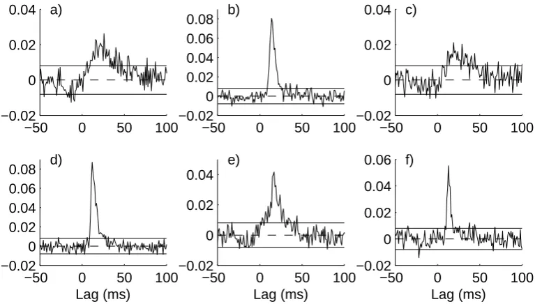
The time domain estimates, ˆρyx(τ), in Figure 6 all have a similar form with a
clear excitatory effect of the gamma inputs onto the primary and secondary sensory endings at positive latencies. There is no consistent evidence in favour of any effects at negative latencies. While there are departures outside the upper and lower 95% confidence intervals at negative latencies, we regard these as chance effects, which should happen on average for 5 points in every 100. As well as confirming the directionality of interaction the plots in figure 6 give some further insight into the dependency of the sensory discharges on the stimulation. The effect of theγs1 input
onto the secondary ending (Fig 6a,c) are longer latency (around +20 ms) and more diffuse than onto the primary ending (Fig 6b,d), which have latencies of +14ms and +12 ms, respectively. The second gamma input, γs2 has a shorter latency onto the
secondary ending, +16 ms (Fig 6e) and a similar latency onto the primary ending, +13 ms (Fig 6f) than the simultaneously activeγs1 input (Fig 6c,d). Taken together
0 50 100 0 0.2 0.4 0.6 a)
0 50 100
0 0.2 0.4 0.6
b)
0 50 100
0 0.2 0.4 0.6
c)
0 50 100
0 0.2 0.4 0.6 Frequency (Hz) d)
0 50 100
0 0.2 0.4 0.6 Frequency (Hz) e)
0 50 100
[image:19.595.114.492.145.388.2]0 0.2 0.4 0.6 Frequency (Hz) f)
Fig. 5. Frequency domain directionality analysis for the same data as described in Table 2. The channel definitions are in column 1 of Table 2. Each panel shows estimates of the original coherence, |Rˆyx(λ)|2 (black trace), and decomposition of this into the forward,|Rˆyx;+(λ)|2 (red trace) and
reverse,|Rˆyx;−(λ)|2(blue trace), directions. The dashed horizontal line is the upper 95% confidence
limit for the coherence estimates, based on the assumption of uncorrelated processes.
−50 0 50 100
−0.02 0 0.02
0.04 a)
−50 0 50 100
−0.02 0 0.02 0.04 0.06 0.08 b)
−50 0 50 100
−0.02 0 0.02
0.04 c)
−50 0 50 100
−0.02 0 0.02 0.04 0.06 0.08 Lag (ms) d)
−50 0 50 100
−0.02 0 0.02 0.04 Lag (ms) e)
−50 0 50 100
−0.02 0 0.02 0.04 0.06 Lag (ms) f)
Fig. 6. Time domain directionality analysis for the same data as described in Table 2. The channel definitions are in column 1 of Table 2. Each panel shows estimates of the correlation measure, ˆρyx(τ).
[image:19.595.113.497.476.694.2]4. Discussion
4.1. General remarks
We have shown how a combined frequency domain and time domain approach can be used to construct non-parametric measures of directionality in bivariate data. Our approach is to combine power spectral density analysis with a MMSE filtering step which reduces the coherency to the cross spectrum. The filtering derives two new processes which have the same correlation structure (coherence and phase) as the original processes, but with spectral densities of 1 at all frequencies. This removes the denominator terms from the coherence function, compare equation (2.1) with equation (2.5). The complex coherency reduces to the cross spectrum of the derived processes, fyxw(ω), allowing the overall correlation, R2yx, to be decomposed using Parseval’s theorem according to time lag, see equations (2.9) and (2.10), which de-compose the total correlation coefficient summatively into three components:R2yx;−,
R2
yx;0 and R2yx;+. These measure the strength of directionality from: x← y, x↔ y
and x → y, respectively, assuming that x is the input process and y the output process. Estimates of the scalar directionality measures have a direct interpretation related to the overall strength of correlation in each direction. A further refinement defined the measures over a restricted frequency range, f α: R2
yx;−,f α, Ryx;0,f α2 and
R2yx;+,f α
The function that we use to derive the directionality measures is the correlation function, ρyx(τ) defined in equation (2.8) as the inverse Fourier transform of the
cross spectrum between the whitened processes, fw
yx(ω). This function captures the
correlation structure in the time domain between the two whitened processes in a similar manner to the way the ordinary cross-covariance (or cumulant density) captures the temporal structure between the original processes as represented in the ordinary cross spectrum, fyx(ω). However, ρyx(τ) is free from any within variable
effects. The whitened processes have the same coherence and phase estimates as the original processes, so all significant features in estimates of ρyx(τ) will reflect the
interaction between the processes, as illustrated in figures 4, 6. In practice numerical issues will result in small differences in the coherence and phase estimates between the original and those for the whitened processes. For the results presented here these differences are less than 10−15 in absolute terms (using MATLAB), there are no practical consequence of these differences for the directionality estimates.
In our case these will be Finite Impulse Response (FIR) filters, typically high pass although the precise form depends on the nature of the electrophysiological signals under consideration. The coefficients of these FIR filters will be symmetrical about the current time sample and will therefore be zero phase filters with no delay (Op-penheim and Schafer, 1975). The filtering process preserves the timing information between the original processes as encoded in the phase estimate. The FIR filters will be non-causal, however, as our processing is done offline, this is not an issue.
The ordinary coherence function, |Ryx(ω)|2, decomposes the overall correlation,
R2yx, as a function of frequency. However, it provides no indication regarding the direction of interaction. To complement the scalar directionality measures we have also introduced a decomposition of the coherence using three frequency domain functions:|R′yx;−(ω)|2,|R′yx;0(ω)|2,|R′yx;+(ω)|2. Estimates of these functions are used to infer directionality at each frequency. These functions decompose the coherence in a summative manner, and thus have an immediate interpretation in terms of the strength of directional interactions at a particular frequency.
The correlation function ρyx(τ) can also be used to provide a visual
represen-tation of the pattern and direction of interaction between the signals. Confidence limits were derived for a NULL hypothesis of no linear dependence, equation (2.41). The interpretation of this measure is similar to a traditional cross-correlation es-timate. One consequence of using the optimal MMSE whitening step is to remove all structure in the input and output signals, thus estimates of ρyx(τ) are a
use-ful addition to the normally used cross-covariance or cumulant density functions in the time domain. The cross covariance function can contain features reflecting the internal structure of one or both of the process (x, y), the MMSE whitening step removes these features. Thus the function ρyx(τ) is likely to be a useful indicator
of the relative timing of between variable effects that is free from within variable effects.
4.2. Summary of results
The non parametric measures were applied to both simulated and real spike train data. Application to the simulated data, section 3.1, demonstrated that all measures correctly inferred the directional interactions between the 3 neurones, as defined in figure 1. The scalar directionality metrics in Table 1 are in agreement with figure 1 as are the estimatedR′ functions in figures 2, 3. The estimates,|Rˆ′
yx;−(λj)|2 and |Rˆ′yx;+(λj)|2 have a direct interpretation in terms of the strength of correlation in
4.3. Relationship with parametric approaches
Much of the previous work on directionality has relied on parametric approaches, where autoregressive models are used to described the random processes and their interactions. We have already commented in the introduction on the issues surround-ing the validity, or otherwise, of ussurround-ing autoregressive models for complex neural data. Notwithstanding this issue, a natural question is to ask how the scalarR2 measures and the magnitude squared R′ functions relate to these previous approaches. Two of the most commonly used measures are those proposed by Granger (1969) and Geweke (1982). Geweke proposed a directional measure to measure linear feedback fromy →xof the formfy→x=loge
(
|Σ1|
|Σ2| )
, where Σ1 is the residual after modelling
process x on its own history, and Σ2 is the residual after modelling process x on
its own history and the history of process y. In the case of no feedback,fy→x = 0,
although in practice negative values can sometimes be obtained (Gersch, 1972). In the Granger framework the measure of the causal effect of y onto x is taken as 1−(|Σ2|
|Σ1| )
, which also has the value 0 in the case of no causal interaction.
Our framework considers the definition of the R2 scalar measures in terms of the coherence function. If the variances, Σ1 and Σ2 in the autoregressive model
are equated to the variance of the output and the residual variance in a linear filter, respectively (Priestley, 1981), then our R2yx directionality measure is equiv-alent to the Granger measure. Extending this argument, then the Geweke feed-back measure could be constructed as fy→x = −loge(1−R2yx
)
, however, as has been pointed out (Lindsay and Rosenberg, 2011) this does not directly measure directional effects as R2
yx is not sensitive to the direction of interaction. A
pos-sible approach here, if Geweke style measures are required, might be to consider the three terms −loge
(
1−R2yx;−)
, −loge
(
1−R2yx;0)
and −loge
(
1−R2yx;+)
as the relevant measures. However, the validity of this suggestion has still to be verified. The present non-parametric approach should be viewed as complementary to the previously discussed parametric methods. In situations well described by low order AR models the Granger (1969) and Geweke (1982) metrics can be used. If there is uncertainty regarding model order, a high model order is required or there are con-cerns regarding the validity of an AR approach, then the non-parametric approach outlined here may be preferable.
4.4. Alternative non-parametric approaches
density estimates. This used a form of normalisation which takes into account the firing rate of the two spike trains. Our approach is similar in concept, but by us-ing the MMSE whitenus-ing step we effectively remove both first and second order (periodic)components from the time domain correlation function ρyx(τ). Thus, all
significant features in time domain plots (e.g fig 4) reflect the interactions between the neurones rather than rhythmic components in the individual spike train firing times.
4.5. Concluding remarks
We have presented a novel approach to estimation of directionality measures that is non-parametric, can be applied to both spike train and time series data (as well as hybrids of the two) and can readily be incorporated into a bivariate spectral analy-sis. The analysis generates two sets of parameters, a scalar set which decomposes the overall strength of correlationR2
yx summatively into three directional components:
R2
yx;−, R2yx;0 and R2yx;+, and a set of functions that decompose the original
coher-ence function |Ryx(ω)|2 summatively into three directional functions: |R′yx;−(ω)|2, |R′yx;0(ω)|2 and|R′yx;+(ω)|2. Estimates of these have a direct interpretation in terms of the strength of correlation (overall or as a function of frequency). A key aspect of our framework is a combined time and frequency domain approach, in the time domain the key parameter is the correlation function ρyx(τ). Use of the MMSE
whitening step removes all within variable effects so that this function characterises only effects between processesx and y.
Areas for further work include development of expressions for confidence limits for theR2 scalar measures and|R′(ω)|2 functions, and exploration of application to a wider range of data. It is recognised that auto regressive based approaches do not scale well (Granger, 1969; Geweke, 1982), a new model has to be constructed for each additional process and the comparison of different auto regressive models can be problematic (Lindsay and Rosenberg, 2011). Future work will explore to what extent non parametric multivariate spectral analysis (Salvador et al., 2005) can be adapted to provide multivariate non-parametric directionality analyses.
5. Software
MATLAB software for non-parametric bivariate directionality analysis is available for free download from the NeuroSpec archive at: http://www.neurospec.org/
References
Baccala LA, Sameshima K (2001). Partial directed coherence: a new concept in neural structure determination. Biological Cybernetics, 84: 463-474.
Bloomfield P (2002) Fourier analyis of time series - An introduction, 2nd ed. John Wiley & Sons Inc. New York.
Bokil H, Purpura K, Schoffelen J-M, Thomson D, Mitra, P (2007). Comparing spectra and coherences for groups of unequal size. Journal of Neuroscience Methods, 159: 337345. Brillinger DR (1972) The spectral analysis of stationary interval functions. In Proc. Sixth
Berkeley Symposium Math. Statist. Probab, (eds. LeCam LM, Neyman J, Scott E) 483-513.
Brillinger DR (1974) Fourier analysis of stationary processes. Proceedings of the IEEE, 62: 1628-1643.
Brillinger DR (1975) Time Series - Data Analysis and Theory. Holt Rinehart & Winston Inc. New York.
Brillinger DR, Lindsay KA, Rosenberg JR (2009) Combining frequency and time domain approaches to systems with multiple spike train input and output. Biological cybernetics, 100: 459-474.
Carvalho R, Buzna L, Bono F, Gutierrez E, Just W, Arrowsmith D (2009) Robustness of trans-European gas networks. Physical Review E 80: 016106.
Chen Y, Bressler SL, Ding M (2006) Frequency decomposition of conditional Granger causal-ity and application to multivariate neural field potential data. Journal of neuroscience methods, 150: 228-237.
Chicharro D (2012) On the spectral formulation of Granger causality. Biological cybernetics, 105: 331-347.
Crespo I, Roomp K, Jurkowski W, Kitano H, del Sol A (2012) Gene regulatory network analysis supports inflammation as a key neurodegeneration process in prion disease. BMC Systems Biology 6: 132.
Daley DJ, Vere-Jones D (2003) An Introduction to the Theory of Point Processes, Vol I: Elementary Theory and Methods. 2nd edition. Springer, Berlin 471pp.
Destexhe A, Rudolph M, Pare D (2003) The high-conductance state of neocortical neurons in vivo. Nature Reviews Neuroscience 4: 739-751.
Dhamala M, Rangarajan G, Ding M (2008a) Analyzing information flow in brain networks with nonparametric Granger causality. NeuroImage, 41: 354-362.
Dhamala M, Rangarajan G, Ding M (2008b) Estimating Granger Causality from Fourier and Wavelet Transforms of Time Series Data. Physical Review Letters, 100: 18701. Diggle, P (1990) Time series : a biostatistical introduction. Clarendon Press, New York. Eichler M, Dahlhaus R, Sandkuhler J (2003) Partial correlation analysis for the identification
of synaptic connections. Biological cybernetics, 89: 289-302.
Eldar YC, Oppenheim AV (2003) MMSE whitening and subspace whitening. IEEE Trans-actions on Information Theory, 49: 1846-1851.
Gersch W (1972) Causality or driving in electrophysiological signal analysis. Mathematical Biosciences, 14: 177-196.
Geweke JF (1982) Measurement of Linear Dependence and Feedback Between Multiple Time Series. Journal of the American Statistical Association, 77: 304-324
Geweke JF (1984) Measures of conditional linear dependence and feedback between time series. Journal of the American Statistical Association, 79: 907-915.
Gladden MH, Matsuzaki H (2002) Staticγ-motoneurons couple group Ia and II afferents of single muscle spindles in anaesthetised and decerebrate cats. Journal of Physiology, 54: 273-288.
Granger CWJ (1969) Investigating Causal Relations by Econometric Models and Cross-spectral Methods. Econometrica, 37: 424-438.
be-tween primary and secondary endings from the same muscle spindle. In: Hnk P, Soukup T, Vejsada R, Zelena (eds)m echanoreceptorsdevelopment, structure and function. Springer, Berlin, pp 225-230.
Halliday DM, Rosenberg JR, Amjad AM, Breeze P, Conway BA, Farmer SF (1995) A frame-work for the analysis of mixed time series/point process data - Theory and application to the study of physiological tremor, single motor unit discharges and electromyograms. Progress in Biophysics and molecular Biology, 64: 237-278.
Halliday DM (2005) Spike-train analysis for neural systems. In: Reeke GN, Poznanski RR, Lindsay KA, Rosenberg JR, Sporns O, editors. Modeling in the neurosciences. 2nd ed. Taylor & Francis pp 555-579.
Jarvis MR, Mitra PP (2001) Sampling properties of the spectrum and coherency of sequences of action potentials. Neural Computation, 13(4): 717-749.
Jeong H, Tombor B, Albert R, Oltvai ZN, Barabasi A-L (2000) The large-scale organization of metabolic networks. Nature 407: 651-654.
Kaiser M (2011), A tutorial in connectome analysis: Topological and spatial features of brain networks, NeuroImage, 57: 892-907.
Kaminski M, Ding M, Truccolo WA, Bressler SL (2001) Evaluating causal relations in neu-ral systems: Granger causality, directed transfer function and statistical assessment of significance. Biological Cybernetics, 85: 145-157.
Karlebach G, Shamir R (2008) Modelling and analysis of gene regulatory networks. Nature Reviews Molecular and Cellular Biology 9: 770-780.
Kendall MG, Stuart A (1961) The advanced theory of statistics, Volume 2. Charles Griffin &Company, London.
Lindsay KA, Rosenberg JR (2011) Identification of directed interactions in networks. Bio-logical cybernetics, 104: 385-396.
McCormick DA (1998) Membrane properties and neurotransmitter actions. In: The synaptic organisation of the brain, 4th edition, ed Shepherd GM. Oxford University Press, Oxford, pp 37-75.
Medkour T, Walden AT, Burgess A (2009) Graphical modelling for brain connectivity via partial coherence. Journal of neuroscience methods, 180: 374-383.
Newman M (2010) Networks: An Introduction (p. 720). Oxford University Press, UK. Olhede SC, Walden AT (2002) Generalized Morse wavelets. IEEE Transactions on Signal
Processing, 50: 2661-2670.
Oppenheim AV, Schafer RW(1975) Digital Signal Processing. Prentice Hall International, UK.
Percival DB, Walden AT (1993) Spectral Analysis for Physical Applications. Cambridge Univ. Press, UK.
Pierce DA (1979) R2 Measures for Time Series. Journal of the American Statistical Associ-ation, 74: 901-910.
Press H, Tukey JW (1956) Power spectral methods of analysis and application in ari-plane dynamics. In The collected works of John W Tukey, Volume 1. Brillinger DR (ed). Wadsworth, California. pp 185-255.
Priestley MB (1981) Spectral analysis and time series. Academic Press, London.
Rigas A (1983) Point Processes and Time Series Analysis: Theory and Applications to Complex Physiological Systems. Ph.D. Thesis, 330pp. University of Glasgow.
Rosenberg JR, Amjad A, Breeze P, Brillinger DR, Halliday DM (1989). The Fourier approach to the identification of functional coupling between neuronal spike trains. Progress in Biophysics and Molecular Biology, 53: 1-31.
neuronal connectivitypartial spectra, partial coherence, and neuronal interactions. Journal of Neuroscience Methods, 83: 57-72.
Rubinov M, Sporns O (2010) Complex network measures of brain connectivity: Uses and interpretations. NeuroImage, 52: 1059-1069.
Salvador R, Suckling J, Schwarzbauer C, Bullmore E (2005) Undirected graphs of frequency-dependent functional connectivity in whole brain networks. Philosophical transactions of the Royal Society of London. Series B, Biological sciences, 360: 937-946.
Schelter B, Winterhalder M, Eichler M, Peifer M, Hellwig B, Guschlbauer B, Lucking CH, Dahlhaus R, Timmer J (2006) Testing for directed influences among neural signals using partial directed coherence. Journal of neuroscience methods, 152: 210-219.
Thomson DJ (1982) Spectrum estimation and harmonic analysis. Proceedings of the IEEE, 70: 1055-1096.
Thomson DJ (1990) Time Series Analysis of Holocene Climate Data. Philosophical Trans-actions of the Royal Society A: Mathematical, Physical and Engineering Sciences, 330: 601-616.
Thomson DJ, Chave A (1991) Jackknifed error estimates for spectra, coherences, and trans-fer functions. In S. Haykin (Ed.), Advances in spectrum analysis and array processing, 1. pp 58-113.
Troyer TW, Miller KD (1997) Physiological Gain Leads to High ISI Variability in a Simple Model of a Cortical Regular Spiking Cell. Neural Computation, 9: 971-983.
Welch P (1967) The use of fast Fourier transform for the estimation of power spectra: a method based on time averaging over short, modified periodograms. IEEE Transactions on Audio and Electroacoustics, 15: 70-73.
Whittaker J (1990) Graphical models in applied multivariate statistics, Wiley, New York. Wilson GT (1972) The Factorization of Matricial Spectral Densities. SIAM Journal on