On Degree-d
Zero-Sum Sets of Full Rank
∗Christof Beierle†, Alex Biryukov, Aleksei Udovenko‡
SnT and CSC, University of Luxembourg, Luxembourg [email protected]
November 25, 2019
Abstract
A set S ⊆Fn2 is called degree-dzero-sum if the sum
P
s∈Sf(s) vanishes for all
n-bit Boolean functions of algebraic degree at mostd. Those sets correspond to the supports of then-bit Boolean functions of degree at mostn−d−1. We prove some results on the existence of degree-dzero-sum sets of full rank, i.e., those that contain
nlinearly independent elements, and show relations to degree-1 annihilator spaces of Boolean functions and semi-orthogonal matrices. We are particularly interested in the smallest of such sets and prove bounds on the minimum number of elements in a degree-dzero-sum set of rankn.
The motivation for studying those objects comes from the fact that degree-d
zero-sum sets of full rank can be used to build linear mappings that preserve special kinds of nonlinear invariants, similar to those obtained from orthogonal matrices and exploited by Todo, Leander and Sasaki for breaking the block ciphers Midori, Scream and iScream.
Keywords: Boolean function, annihilator, orthogonal matrix, nonlinear invari-ant, trapdoor cipher, symmetric cryptography
1
Introduction
After the introduction oflinear cryptanalysisin [13] as a powerful method to attack sym-metric cryptographic primitives, people started studying how to generalize this method in order to exploit nonlinear approximations for cryptanalysis, see, e.g., [6] and [11]. While it might be easier to find a nonlinear approximation over parts of the primitive, e.g., over an S-box of small size, a crucial problem in nonlinear cryptanalysis is to find nonlinear approximations that hold true for the whole round function of the primitive.
∗This is a pre-print of an article published in Cryptography and Communications. The final
authen-ticated version is available online at: https://doi.org/10.1007/s12095-019-00415-0
†The work of Christof Beierle was funded by theSnT Cryptolux RG budget.
‡The work of Aleksei Udovenko was funded by the Fonds National de la Recherche Luxembourg
An example that exploits nonlinear approximations that are preserved over the whole round function is bilinear cryptanalysis over Feistel ciphers [4].
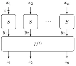
More recently, an interesting solution for the above problem was described by Todo, Leander and Sasaki in [18] for round functions that can be described in terms of an LS-design [5]. Let one round of a substitution-permutation cipher operating on n S-boxes of t-bit length be given as depicted in Figure 1 and let the linear layer L(t):
Fnt2 → Fnt2
only XOR the outputs of the S-boxes, i.e., each (y1, . . . , yn) for yj ∈ Ft2 is mapped to
(z1, . . . , zn) where zj = Pni=1αi,jyi for particular αi,j ∈ F2. In that case, L(t) can be
defined by
L=
α1,1 α1,2 . . . α1,n
α2,1 α2,2 . . . α2,n
..
. ... . .. ...
αn,1 αn,2 . . . αn,n
.
Todo et al. observed that if L is orthogonal, then for any t-bit Boolean function f of algebraic degree less than or equal to 2 it is
f(y1) +f(y2) +· · ·+f(yn) =f(z1) +f(z2) +· · ·+f(zn). (1)
This fact was used to successfully cryptanalyze the block ciphers Midori, Scream and iScream in a weak key setting. Indeed, iff is any invariant function for the S-boxS, i.e., if for all x ∈Ft2, f(x) =f(S(x)), and if deg(f) ≤2, one obtains an invariant function
for the whole round according to Equation 1.
An interesting question is whether the property of Lbeing orthogonal is also neces-sary for Equation 1 to hold for allf with degree upper-bounded by 2. More generally, we would like to understand the necessary and sufficient properties of the linear layer that preserve such invariants in the case when deg(f)≤dford >2. Although the existence of a non-trivial1 linear layer for which Equation 1 holds for allf with degf ≤dis totally unclear, such a construction would be of significant interest. On the one hand, it would deepen the knowledge on how to design strong symmetric cryptographic primitives and to avoid possible attacks and could on the other hand be useful in order to design sym-metric trapdoor ciphers to be used as public-key schemes, see, e.g., [2, 15, 17]. The idea would be to hide a nonlinear approximation as the trapdoor information. If the linear layer is designed such that it preservesall invariants of a special form, e.g., all functions of degree at mostd, the specification of the linear layer would not leak more information on the particular invariant and thus on the trapdoor. There could also be applications besides cryptography, so the above problem might be of independent interest.
1.1 Our Contribution
In this work we answer the above question and consider the case of L∈Fn2×m, i.e., the number of outputs (m) might be different than the number of inputs (n). We precisely
S S S
L(t)
. . .
x1 x2 xn
z1 z2 zn
y1 y2 yn
t
Figure 1: The round function of a substitution-permutation cipher based on an LS-design.
characterize the matrices that preserve all invariants of the form similar as given in Equation 1, i.e.,
f(y1) +· · ·+f(yn) =f(z1) +· · ·+f(zm) +f(0)·(m+n mod 2), (2)
where the degree of f is upper bounded by dand we call such matrices degree-d sum-invariant. We show that such matrices can be build from zero-sum sets of rankn, i.e., they correspond to then-bit Boolean functions of degree at mostn−d−1 which admit no linear annihilator. This characterization is obtained in Propositions 2, 3 and 4. Our results imply that m ≥ n and, for the case of d = 2, the property of L being (semi-)orthogonal is not only sufficient, but also necessary. Moreover, we obtain an interesting characterization of orthogonal matrices overF2, i.e., L∈Fn2×n is orthogonal if and only
if in every 2×2nsubmatrix of In L
, each column occurs an even number of times. Besides showing the link between degree-dzero-sum sets and degree-dsum-invariant matrices, we study degree-dzero-sum sets of full rank in more detail. We are in particular interested in the smallest of such sets. Let F(n, d) denote the minimum number of elements in a degree-d zero-sum set of rank n. The following theorem summarizes our main results.
Theorem 1. Let n, d ∈ N with n > d ≥ 1. Then the following properties of F(n, d)
hold.
(i) F(n, d) = min{wt(g)|g∈ Bn,n−d−1\ {0} with dim AN1(g)≤1}.
(ii) F(n,1) =n+ 2−(n mod 2) and, for n= 4 or n >5, F(n,2) = 2n.
As exceptions, F(3,2) = 8 and F(5,2) = 12.
(iii) F(d+ 1, d) =F(d+ 2, d) = 2d+1. Moreover, F(d+ 3, d) = 3·2d andF(2d+ 4, d) = 2d+2. For d+ 4≤n≤2d+ 3,
F(n, d) = 22d−n+4(2n−d−2−1).
(v) for n1, n2 > d, the inequality
F(n1+n2, d)≤F(n1, d) +F(n2, d)
holds. Moreover, ford≥2, it is
F(n+d, d−1)≤F(n, d)≤2F(n−1, d−1).
The last inequality implies that, for n≥4, F(n,3)≥2n+ 6.
We prove the above values by providing a construction of the corresponding zero-sum sets (resp. Boolean functions). In case where we only prove an upper bound, we provide a construction that meets this bound. Table 1 shows the values and bounds for F(n, d) forn≤30 andd≤10.
The last inequality in Theorem 1 implies that any degree-d sum-invariant matrix
L∈ Fn2×n ford≥3 must be a permutation matrix. In other words, the observation of Todoet al. cannot be extended for higher-degree invariants withoutLbeing expanding.
1.2 Organization
In Section 2, we fix our notation and recall basic properties of Boolean functions. We also recall the observations made in [18] with regard to orthogonal matrices and the preservation of degree-2 invariants. For motivating the remainder of the paper, we directly present an example construction of an expanding linear mapping that preserves higher-degree invariants.
In Section 3, we show equivalent characterizations of degree-d zero-sum sets and explain the links between degree-dsum-invariant matrices and degree-dzero-sum sets.
We study minimal degree-dzero-sum sets in Section 4 and prove the results summa-rized in Theorem 1. We further summarize the implications to degree-d sum-invariant matrices in Section 5. Finally, the paper is concluded in Section 6.
2
Preliminaries
ByNwe denote the set of natural numbers{1,2, . . .}and byF2 we denote the field with
two elements, i.e.,{0,1}. We represent elements inFn2 as row vectors and we denote by
ei thei-th unit vector. For a vectoru= (u1, . . . , un)∈Fn2 let wt(u) :=|{i∈ {1, . . . , n} |
ui = 1}|denote theHamming weight ofu. For a Boolean functionf, we denote by wt(f)
the Hamming weight of the value vector of f. For a setS ⊆ Fn2, the indicator of S is
defined as the Boolean function 1S :Fn2 →F2 for which 1S(x) = 1 if and only if x∈S.
LetBn,d denote the set ofn-bitBoolean functions f:Fn2 →F2 of algebraic degree at
most d. Any Boolean function f ∈ Bn,d can be uniquely represented as a multivariate
polynomial in F2[x1, . . . , xn]/(x21+x1, . . . , x2n+xn) through its algebraic normal form (ANF). That is,
f(x) = X
u∈Fn
2
where x = (x1, . . . , xn), u = (u1, . . . , un) and xu := Qni=1xuii. Because the algebraic
degree is upper bounded by d, it is au = 0 for all u with wt(u) > d. Any Boolean
function with algebraic degree at most 1 is said to be affine and an affine function f
with f(0) = 0 is said to be linear. The algebraic degree of the zero-function is defined to be−∞. We use the symbolto denote the partial ordering on Fn2 defined byxu
if and only if, for alli∈ {1, . . . , n},xi≤ui.
For any two vectors x, y ∈ Fn2, we denote by xy := (x1y1, . . . , xnyn) ∈ Fn2 the Hadamard product of x and y. The inner product of x and y is given by
hx, yi:=
n X
i=1
xiyi = wt(xy) mod 2.
We generalize this notion to one vector or more than two vectors in the following sense. Letx1, . . . , xd∈Fn2. Then we define
hx1, . . . , xdi:= n X
i=1 d Y
j=1
xj,i= wt(x1 · · · xd) mod 2.
We use Fn2×m to denote the set of matrices inF2 with nrows and m columns. The
n×n identity matrix will be denoted by In. Any matrix L ∈ Fn2×m defines a linear
mapping ϕ: Fn2 → Fm2 , x 7→ xL. We denote by L> the transpose of the matrix L. Li
denotes thei-th row ofL.
2.1 Higher-Order Derivatives, Affine Equivalence and Algebraic Im-munity of Boolean Functions
For a Boolean function f :Fn2 →F2 and a vector α∈Fn2, we denote the functionδαf : Fn2 →F2 to be thederivative off with respect toα, given byδαf(x) :=f(x) +f(x+α).
It is well known that degδαf ≤degf−1 for any Boolean functionf and anyα, see [12].
The derivation can be iterated multiple times resulting in ahigher-order derivative. For
dlinearly independent vectorsα1, . . . , αd∈Fn2 it holds that
δα1. . . δαdf(x) =
X
z∈span(α1,...,αd)
f(x+z).
If the vectorsα1, . . . , αd are linearly dependent, then the derivative is equal to zero.
Boolean functions have several applications in cryptography, e.g., for designing stream ciphers. In order to resist algebraic attacks, the notion of algebraic immunity was intro-duced in 2004 as follows.
Definition 1 (Algebraic immunity [14]). Let f:Fn2 → F2. An n-bit Boolean function
g 6= 0 is called an annihilator of f, if f g = 0. The set of annihilators of f together withg= 0 forms a vector space, denoted by AN(f). We denote byANd(f) the subspace of annihilators of f with algebraic degree at most d together with the zero-function. The algebraic immunity of f, denoted AI(f), is defined as the minimum k for which
An important concept for Boolean function is the notion of affine equivalence.
Definition 2 (Affine Equivalence). Two Boolean functions f, g:Fn2 → Fn2 are called
affine equivalent if there exists a linear bijectionϕ:Fn2 →Fn2 and a vector c ∈Fn2 such thatg=f◦(ϕ+c). If c= 0, f andg are called linear equivalent.
It is well known that the weight, the algebraic degree and the dimensions of the anni-hilator spaces (and thus the algebraic immunity) are invariant under affine equivalence.
2.2 Orthogonal Matrices and Preservation of Nonlinear Invariants
In [18], Todo, Leander and Sasaki introduced thenonlinear invariant attack and success-fully distinguished the block ciphers Midori, Scream and iScream from a random per-mutation for a significant fraction of weak keys. For ann-bit permutationG:Fn2 →Fn2,
the main idea consists in finding a non-constantn-bit Boolean functionf and a constant
ε∈F2 such that
∀x∈Fn2:f(x) =f(G(x)) +ε .
Such a function f is called an invariant for G. In order to find an invariant for the cipher, Todo et al. observed that if L ∈ Fn2×n is an orthogonal matrix, i.e., if
hxL, yLi=hx, yifor all x, y∈Fn2, then for all Boolean functionsf ∈ Bt,2 it is
∀X ∈Ft2×n:
n X
i=1
f (X>)i
=
n X
j=1
f ((XL)>)j
. (3)
In other words,any Boolean functionf:Ft2 →F2 of algebraic degree at most 2 gives
rise to an invariant over the linear layers of Midori, Scream and iScream of the form (x1, . . . , xn) 7→ f(x1) +· · ·+f(xn), where n denotes the number of S-boxes, t denotes
the bit length of the S-box andxi ∈Ft2.
We illustrate this from a slightly different point of view on the example of the linear layer used in Midori (see [1]), which is defined by the following matrix:
L=
0 1 1 1
1 0 1 1
1 1 0 1
1 1 1 0
. (4)
It is easy to see thatLis orthogonal. Thus, according to Equation 3, foranyf ∈ Bt,2
and allx1, x2, x3, x4 ∈Ft2, the following equation holds:
f(x1) +f(x2) +f(x3) +f(x4) =
f(x2+x3+x4) +f(x1+x3+x4) +f(x1+x2+x4) +f(x1+x2+x3).
We now consider an alternative way of proving this. The arguments of f form an affine subspace of dimension 3, namely x1+ span(x1+x2, x1+x3, x1+x4). Therefore,
the equation is equivalent to
which is clearly true for anyf ∈ Bt,2and anyx1, x2, x3, x4since all third-order derivatives
of a quadratic function are equal to zero. This observation gives new insights on how to generalize the linear layer in order to preservehigher-degree invariants.
Proposition 1. Let d ≥ 2 be an integer. Then there exists a matrix L ∈ Fn2×m with
n=d+ 2, m= 2d+1−d−2 and full rank n such that for any t≥1 and any f ∈ Bt,d, the following property holds:
∀X ∈Ft2×n:
n X
i=1
f (X>)i
=
m X
j=1
f ((XL)>)j
. (6)
An example of such L is given by a matrix with columns taken as all vectors from Fn2 with an odd Hamming weight greater or equal to 3.
Proof. For any t≥1 and any x0, . . . , xd+1 ∈Ft2 consider the (d+ 1)-dimensional affine
subspace
V =x0+ span(x0+x1, x0+x2, . . . , x0+xd+1).
For any Boolean functionf of degree d, any (d+ 1)-th derivative vanishes. Therefore,
P
v∈V f(v) = 0. This can be equivalently written as
f(x0) +f(x1) +. . .+f(xd+1) =
= X
I⊆{1,...,d+1} |I|≥2 even
f(x0+ X
i∈I
xi) +
X
I⊆{1,...,d+1} |I|≥3 odd
f(X
i∈I
xi)
= X
I⊆{0,...,d+1} |I|≥3 odd
f(X
i∈I
xi).
(7)
The right-hand side contains 2d+1−d−2 applications of f. Let Y be the set of the linear functions defining the arguments off in the right-hand side of Equation 7, i.e.,
Y =
( X
i∈I
xi
I ⊆ {0, . . . , d+ 1}, |I| ≥3 odd
)
,
and let Lbe the matrix corresponding to the linear function mapping (x0, x1. . . , xd+1)
to (y1, y2. . . , y2d+1−d−2), whereyi∈Y and allyiare pairwise different. Then, Equation 7
is equivalent to Equation 3 with the describedL.
Since m ≥ n ≥ 4, any unit vector from Fn2 can be expressed a linear
combina-tion of 3 columns of L, e.g., (1,0,0,0, . . . ,0) = (1,1,1,0, . . . ,0) + (1,0,1,1, . . . ,0) + (1,1,0,1, . . . ,0). We conclude thatL has full rank n.
Example 1. Ford= 2 we obtain the orthogonal matrix given in Equation 4. Ford= 3
matrixL:
L=
0 0 0 0 1 1 1 1 1 1 1
0 1 1 1 0 0 0 1 1 1 1
1 0 1 1 0 1 1 0 0 1 1
1 1 0 1 1 0 1 0 1 0 1
1 1 1 0 1 1 0 1 0 0 1
.
3
Degree-d
Zero-Sum Sets and Sum-Invariant Matrices
A natural question to ask is which other linear mappings have a similar property as given in Equation 6. To answer this question, we study degree-d zero-sum sets as a generalization of the above problem.
Definition 3 (Degree-d Zero-Sum Set). Let S ⊆ Fn
2 and let d ∈ N. We call S to be
degree-dzero-sumif, for all f ∈ Bn,d,
X
s∈S
f(s) = 0. (8)
We define rank(S) to be the maximum number of linearly independent elements in S
and denote byZSdn×m the set of degree-d zero-sum sets with m elements and rank n.
We first show the following equivalent characterizations of degree-dzero-sum sets.
Proposition 2. LetS ={s1, . . . , sk} ⊆Fn2 and let d∈N. LetMS ∈Fn
×k
2 be any matrix (up to a permutation of the columns) the columns of which correspond to the elements of S, i.e., MS = s>1 . . . s>k
. Then the following statements are equivalent:
(i) S is a degree-d zero-sum set.
(ii) kis even and, for any choice of d(not necessarily distinct) rowsr1, . . . , rdof MS, it is hr1, . . . , rdi= 0.
(iii) in every d×k submatrix ofMS, each column occurs an even number of times.
(iv) deg(1S)≤n−d−1.
(v) for allt≥1 and all f ∈ Bt,d, ∀X ∈Ft×n 2 :
P
s∈Sf(sX>) = 0.
In particular, the degree-d zero-sum sets in Fn2 are exactly the supports of the n-bit Boolean functions of degree at most n−d−1. Therefore, any non-empty degree-d zero-sum set must contain at least2d+1 elements.
Proof. To prove (i)⇒(ii), let
MS =
r1
.. .
rn
with ri ∈ Fk2. Let l1, . . . , ld bed (not necessarily distinct) row indices and consider the
monomial function f ∈ Bn,d, x 7→ Qd
i=1xli, which has degree d. From Equation 8, it
must be
0 =X
s∈S
f(s) =X
s∈S d Y
i=1
sli =hrl1, . . . , rldi.
Clearly,kmust be even because P
s∈S1 = 0.
(ii) ⇒ (iii): We first see that any 1×k submatrix of MS contains each element in F2 an even number of times. Indeed, let r be any row inMS. From (ii) we know that
wt(r) mod 2 =hri= 0 and thusr contains an even number of 1’s. Becausekis even, it must also contain an even number of 0’s. We now use induction on the number of rows. Let d0 < d such that (ii) ⇒ (iii) holds for d0. Let us choose an arbitrary (d0+ 1)×k
submatrixH= [mi,j]1≤i≤d0+1,1≤j≤kofMS. We defineH(0) := [m(0)
i,j] to be the submatrix
ofH that is obtained by selecting exactly the columnsm?,j of H for whichmd0+1,j = 0.
Similarly, letH(1) := [m(1)
i,j] be the submatrix of H that is obtained by selecting exactly
the columnsm?,j ofH for whichmd0+1,j = 1. We have already seen from the initial step
that both H(0) and H(1) must contain an even number of columns (otherwise the row
md0+1,? would have an odd weight). From (ii), we know that
0 =hm1,?, . . . , md0,?, md0+1,?i=hm(0)
1,?, . . . , m (0)
d0+1,?i+hm (1)
1,?, . . . , m (1) d0+1,?i
=hm(1)1,?, . . . , m(1)d0,?i=hm (0)
1,?, . . . , m (0) d0,?i.
Because of the induction hypothesis,H(0)andH(1)contain each column an even number
of times and therefore, every column of H occurs an even number of times.
(iii) ⇒(iv): Let u ∈ Fn2 with wt(u) ≥n−d. Because of (iii), |{s∈ S |s u}| is
even. It follows that
|{s∈S |su}| mod 2 =X
su
1S(s) = 0
and thus, the monomial xu doesn’t occur in the ANF of 1
S. Since this holds for all u
with wt(u)≥n−d, the algebraic degree of 1S is at most n−d−1.
(iv)⇒(v): Letf ∈ Bt,dbe an arbitrary function of degree at most d. Observe that
∀X∈Ft2×n X s∈Fn2
1S·f(sX>) = 0, (9)
because deg1S·(f ◦X)≤deg1S+ degf ≤n−1. Here,f◦Xdenotes then-bit Boolean
functions7→f(sX>). Equation 9 can equivalently be written as
∀X∈Ft2×n X s∈S
f(sX>) = 0,
which proves (v). The implication (v)⇒(i) follows by lettingt=nand X =In.
It is worth remarking that the property of being degree-dzero-sum is invariant under the application of an injective linear mapping. Indeed, ifϕ: span(S)→Fn0
2 is an injective
linear function on the subspace span(S) of dimension rank(S), then |ϕ(S)|=|S|and if
S is degree-dzero-sum, so is ϕ(S). Further, rank(ϕ(S)) = rank(S). Therefore, without loss of generality, we can represent a zero-sum set S ∈ ZSdn×m as a subset of Fn2 and
given by the columns of an n×m matrix MS of the form
MS = In L
(10)
for an L ∈ Fn2×(m−n). We say that a zero-sum set (resp. a matrix MS) given in the
representation of Equation 10 is insystematic form. We are in particular interested in the properties of such matricesL that define zero-sum sets in ZSdn×m in the above way.
For instance, such an L can only exist if m is even. We generalize this by introducing the notion of adegree-dsum-invariant matrix as follows.
Definition 4 (Degree-dSum-Invariant Matrix). A matrixL∈Fn2×m is called degree-d
sum-invariant if, for allt≥1 and all f ∈ Bt,d,
∀X ∈Ft2×n:
n X
i=1
f (X>)i
=
m X
j=1
f ((XL)>)j
+εm+nf(0), (11)
where εm+n= (m+n) mod 2.
Proposition 3. Let L ∈Fn2×m be a linear mapping and let d∈N. Then the following statements are equivalent:
(i) L is degree-dsum-invariant.
(ii) The columns of the matrix dML occurring with odd multiplicity define a degree-d zero-sum set, where
( d
ML:= In L
∈F2n×(m+n), if m+n is even;
d
ML:= In L 0
∈F2n×(m+n+1), if m+n is odd. (12)
(iii) For all x1, . . . xd∈Fn2 it is hx1, . . . , xdi=hx1L, . . . , xdLi.
Moreover, if L fulfills (i) and if d ≥ 2, then n ≤ m, LL> = In and L must have full rank n.
Proof. We first prove (i)⇒(ii). Ifm+nis even, then Equation 11 is equivalent to
∀X∈Ft×n 2 :
n X
i=1
f eiX>
+
m X
j=1
f (L>)jX>
= 0, (13)
where ei denotes the i-th unit vector. If there is a j for which (L>)j is equal to a
Similarly, if there exist two differentj1, j2 such that (L>)j1 = (L
>)
j2, thenf((L
>)
j1X
>)
and f((L>)j2X
>) cancel out. This is another way of saying that the columns of the
matrix dML =
In L
occurring with odd multiplicity define a degree-d zero-sum set.
If m+nis odd, then εm+n= 1 and Equation 11 can be written as
∀X∈Ft2×n:
n X
i=1
f eiX>
+
m X
j=1
f (L>)jX>
+f(0X>) = 0.
This is equivalent to say that the columns of the n ×(m +n + 1) matrix dML =
In L 0
occurring with odd multiplicity define a degree-dzero-sum set.
(ii) ⇒ (iii). If the columns of MLd occurring with odd multiplicity define a
degree-d zero sum set, then, because of Proposition 2, any d (not necessarily distinct) rows [el1 |Ll1], . . . ,[eld |Lld] of MLdfulfill
h[el1 |Ll1], . . . ,[eld|Lld)]i= 0,
which is equivalent to hel1, . . . , eldi = hel1L, . . . , eldLi. Because of the linearity of the
inner product, i.e.,hx1+x01, x2, . . . , xdi=hx1, x2, . . . , xdi+hx01, x2, . . . , xdi, the statement
follows.
(iii)⇒(i). If there aref1, f2∈ Bt,d such that Equation 11 holds for bothf1 andf2,
then it clearly holds forf1+1 and forf1+f2as well. Therefore, without loss of generality,
let f ∈ Bt,d be a monomial function, i.e.,f(z) =Qd
k=1zlk for 1≤l1 ≤ · · · ≤ld≤t. Let
X∈Ft2×n. Then,
n X
i=1
f((X>)i) = n X
i=1 d Y
k=1
(X>)i,lk =hXl1, . . . , Xldi
and
m X
j=1
f(((XL)>)j) +εm+nf(0) = m X
j=1 d Y
k=1
((XL)>)j,lk =hXl1L, . . . , XldLi.
It follows that if L preserves all generalized inner products of d elements, then L is degree-dsum-invariant.
If Lfulfills the equivalent statements (i) - (iii), then, for allx, y∈Fn 2, it is
xy>=hx, yi=hxL, yLi=xL(yL)>=xLL>y .
It follows that LL> must be the identity and thus, L must have full rankn.
This result shows a relation between degree-d sum-invariant matrices and semi-orthogonal matrices. A matrix L ∈ Fn2×m with n ≤ m is called semi-orthogonal if
LL>=I
it is semi-orthogonal.2 Because of the above relation, the degree-(d+ 1) sum-invariant matrices might also be called d-th order semi-orthogonal.
The invertible semi-orthogonal matrices are exactly the orthogonal matrices and the orthogonal matrices in dimension n form a multiplicative group, called the orthogonal group. With the above equivalences, we obtain an interesting characterization of the orthogonal groups over F2.
Corollary 1. A matrix L∈Fn2×n is orthogonal if and only if in each2×2nsubmatrix of
In|L
, each column occurs an even number of times.
3.1 Relation to Orthogonal Arrays
Proposition 2 points out a relation between degree-dzero-sum sets and orthogonal arrays.
Definition 5 (Orthogonal Array [7]). An m×n matrix M with entries from a finite set of cardinalityk is said to be an orthogonal array withklevels, strengthdand index
λ, denoted OA(m, n, k, d), if every m×dsubmatrix of M contains each d-tuple exactly
λ times as a row. Without loss of generality, we will assume that M is a matrix with elements inZk.
For our purposes we are only interested in the case ofk= 2. We directly obtain the following.
Corollary 2. Let S⊆Fn
2. If M>S is an OA(|S|, n,2, d) such that 2d+1 divides |S| (i.e., if the index λis even), then S is a degree-dzero-sum set.
As an example, for d = 3, there is a well-known construction of orthogonal arrays from Hadamard matrices (see, e.g., [7, pp. 145–148]). AHadamard matrix of ordernis a matrixH∈Zn×nwhich can only take values in{−1,1}and which fulfillsH>H =nIn.
For a matrixM with elements in{−1,1}, we denote byMftheF2 matrix obtained from
M by replacing−1 with 0, i.e., we defineMfto be the result of 12(M+ 1), interpreted in F2.
If H is a Hadamard matrix of order 8kfork∈N, it is well known that
^
H
−H
is an OA(16k,8k,2,3) of even index (see [8, Theorem 4.16]). Therefore, it defines a degree-3 zero-sum set S⊆F8k
2 with 16kelements. However, its rank can be at most 4k
(see [16, Proposition 2]) and we are interested in the zero-sum sets of full rank.
2
We only consider matrices with n ≤ m. If L ∈ F2n×m with n > m, L would be defined to be
4
Minimal and Maximal Zero-Sum Sets
In this section we study zero-sum sets of particular rank n and prove results on their existence. We are particularly interested in the smallest of such sets, defined in the following sense.
Definition 6. We denote by F(n, d) the minimum number m ∈ N for which there exists an S ∈ZSdn×m. We call a zero-sum set minimal if it is contained in ZSdn×F(n,d). Analogously, a zero-sum setS ∈ZSdn×m is called maximal ifZSdn0×m=∅for alln0 > n.
Note that F(n, d) is only defined if n > d as otherwise, the only degree-dzero-sum set inFn2 is the empty set. We first characterize the zero-sum sets of particular rankn
in terms of Boolean functions.
4.1 Relations between Zero-Sum Sets and Affine Annihilators of Boolean Functions
The first three existence results are presented in Propositions 4, 5 and 6 and outline the link between zero-sum sets and the dimensions of degree-1 annihilator spaces of Boolean functions.
Proposition 4. There exists a degree-d zero-sum set S ∈ ZSdn×m if and only if there exists a Boolean function h∈ Bn,n−d−1 with wt(h) =m and dim AN1(h)≤1.
Proof. Let us assume that S ∈ ZSdn×m is given in systematic form, i.e., it can be
rep-resented as in Equation 10. Then, S = supp(h) for a Boolean function h ∈ Bn,n−d−1
for which ∀i∈ {1, . . . , n}:h(ei) = 1. Such a function cannot have a linear annihilator
and therefore, anya∈AN1(h)\ {0} must be of the forma=`+ 1 for a linear Boolean
function`. It follows that dimAN1(h)≤1.
Let now h ∈ Bn,n−d−1 with wt(h) =m and dim AN1(h)≤1. Leta∈AN1(h)\ {0}.
Ifa=`+ 1 for a linear function`, thenhhas no linear annihilator. Ifais linear, we fix a constantc∈Fn
2 for whicha(c) = 1 and consider the functionhc:x7→h(x+c)∈ Bn,n−d−1
which is affine-equivalent to h and thus has the same weight. It is easy to verify that
a+ 1 is an affine annihilator forhc. Because the dimensions of the annihilator spaces are
invariant under affine equivalence,hchas no linear annihilators. Therefore, without loss
of generality, we can assume that h has no linear annihilator. LetS= supp(h)⊆Fn 2 be
the support of h and consider a matrixMS the columns of which form exactly the set
S. Sinceh has no linear annihilator, there is no linear combination of rows of MS that
is equal to zero. We conclude thatMS has full rank nand S ∈ZSdn×m.
Proposition 5. Given a function h ∈ Bn,n−d−1 with wt(h) =m and AN1(h) ={0}, it is possible to construct a zero-sum set inZSd(n+1)×m.
Proof. Consider the function
Note thath0 has degree at mostn−d. Further, h0 has no linear annihilator. Otherwise, by setting xn+1 = 1, we would obtain that h has an annihilator of algebraic degree 1,
contradicting AN1(h) ={0}. By Proposition 4, we can construct S∈ZSd(n+1)×m.
A converse statement is true for maximal zero-sum sets.
Proposition 6. Let n ≥ 2 and let S ∈ ZSd(n+1)×m be maximal. Then, 1S is linear equivalent to a functionh∈ Bn+1,n−d of the form
h(x1, . . . , xn+1) =xn+1·g(x1, . . . , xn), (14)
where g ∈ Bn,n−d−1 with wt(g) = wt(h) =m and AN1(g) ={0}. Further, ifm <2n−1, thenAI(g)≥2.
Proof. Let MS be a matrix which columns correspond to the elements ofS. Because S
is maximal, the vector subspace ofFm2 spanned by the rows ofMS must contain the all-1
vector 1m := (1,1, . . . ,1). Otherwise, one would obtain a zero-sum set in ZSd(n+2)×m
defined by the matrix
MS
1m
.
Therefore, we can apply a linear permutationAon the columns ofMS such that1A(S)=
h where h ∈ Bn+1,n−d is of the form as given in Equation 14 with g ∈ Bn,n−d−1 and
wt(g) = wt(h). It is left to show that AN1(g) ={0}.
Clearly,gcannot have a linear annihilator. We assume now thatghas an annihilator of degree 1 of the form (x1, . . . , xn) 7→ 1 +Pni=1aixi. Then, g(x) = 0 for all x with Pn
i=1aixi = 0. Let j be such that aj = 1. For the linear permutation Q : Fn2 → Fn2,
Q(x1, . . . , xn) = (x1, . . . , xj−1,Pni=1aixi, xj+1, . . . , xn), we have
g(Q(x1, . . . , xn)) =xj ·g0(x1, . . . , xj−1, xj+1, . . . , xn)
for a functiong0 ∈ B
n−1,n−d−2. But this means that h is linear-equivalent to a function
of the form (x1, . . . , xn+1) 7→xn+1·xn·g0(x1, . . . , xn−1), which has a linear annihilator
xn+1+xn. We get a contradiction and conclude that AN1(g) ={0}.
If m < 2n−1, it is easy to see that g+ 1 cannot admit an annihilator of algebraic degree 1. Suppose thata∈AN1(g+ 1)\ {0}. Then, wt(a) = 2n−1 and ag=a, which is
impossible.
As Proposition 6 only holds for maximal zero-sum sets we cannot use it to establish an equivalence between minimal degree-d zero-sums of rank n+ 1 and n-bit Boolean functions of degree n−d−1 with algebraic immunity at least 2 and minimum weight. We therefore propose the following question:
4.2 Minimal Zero-Sum Sets: Bounds and Values for F(n, d)
In order to derive values for F(n, d), we basically have to study the Boolean functions that admit at most one annihilator of algebraic degree 1 and find those of minimum weight. Indeed, from Proposition 4, we know that
F(n, d) = min{wt(g)|g∈ Bn,n−d−1\ {0} with dim AN1(g)≤1}.
For d = 1 and d= 2 we can easily determine the cardinalities of minimal degree-d
zero-sum sets, as stated in Propositions 7 and 8. The proofs also provide a construction for a minimal zero-sum set. While the proof ford= 1 is rather trivial, the proof ford= 2 relies on the relation between degree-2 zero-sum sets and semi-orthogonal matrices.
Proposition 7. Forn≥2, F(n,1) =n+ 2−(n mod 2).
Proof. Consider a zero-sum setS ∈ZS1n×m and its matrix in systematic form. Each row must have an even weight, therefore there must be at least one extra column besides the identity part, i.e. m ≥ n+ 1. Furthermore, m must be even and the proposition follows.
Proposition 8. For n= 4 and for n >5, it is F(n,2) = 2n. Further, F(3,2) = 8 and
F(5,2) = 12.
Proof. Let n≥3 and m be minimal such that there exists anS ∈ZS2n×m. Let further
L ∈ Fn2×(m−n) such that S is in systematic form with MS = [In|L]. As MS cannot
contain any repeated columns, it isMS =MLdand thus, Lmust be semi-orthogonal and
n≤(m−n). It follows thatF(n,2) =m≥2n.
Let now n= 4 or n≥6. To prove the existence of anS ∈ZS2n×2n, we observe that
if L ∈ Fn2×n is an orthogonal matrix for which each column has weight larger than 1,
d
ML defines a degree-2 zero-sum set of size 2n and rank n according to Proposition 3.
It is left to show that, for any dimension n = 4 or n ≥ 6, there exists an orthogonal matrix for which no column corresponds to a unit vector. We are going to distinguish four cases. Let us define the orthogonal matrices M4 and M6 as
M4=
0 1 1 1
1 0 1 1
1 1 0 1
1 1 1 0
, M6=
0 1 1 1 1 1
1 0 1 1 1 1
1 1 0 1 1 1
1 1 1 0 1 1
1 1 1 1 0 1
1 1 1 1 1 0
.
Case 1 (n= 0 mod 4): The block-diagonal matrix diag(M4, . . . , M4) which contains
M4 as its diagonal blocks is orthogonal and each column weight is equal to 3.
Case 3 (n= 3 mod 4): Becausen >5, it isn= 4k+3 fork≥1 and the two matrices
D1 = diag(1,1,1, M4, M4, . . . , M4) andD2= diag(M4,1,1, . . . ,1) are orthogonal. Their
product is orthogonal and of the form
D1D2 =
0 1 1 1
1 0 1 1
1 1 0 1
0 0 . . . 0 0 0 . . . 0 0 0 . . . 0
A
D
, (15)
whereD is the 4k×(4k−1) submatrix of diag(M4, . . . , M4) omitting the first column.
It is obvious that each column has weight at least 3.
Case 4 (n = 1 mod 4): Because n > 5, it is n ≥ 9 and n= 4k+ 6 + 3 for k ≥0. The two matrices D1 = diag(1,1,1, M6, M4, . . . , M4) and D2 = diag(M4,1,1, . . . ,1) are
orthogonal. Their product is orthogonal and of the form given in Equation 15 with D
as the (4k+ 6)×(4k+ 6−1) submatrix of diag(M6, M4, M4, . . . , M4) omitting the first
column. It is obvious that each column has weight at least 3.
Forn= 3 we use that any degree-dzero-sum set must contain at least 2d+1 elements. Thus,F(n,2)≥8. We obtainF(3,2) = 8 because F32 is a degree-2 zero-sum set.
For n= 5, assume that there exists an orthogonal matrix L∈F52×5 which does not have a unit vector as its row (or column). From point (iii) of Proposition 2 it follows that any 2×5 submatrix of Lmust contain an odd number of columns equal to each of (0,1),(1,0),(0,0) and an even number of columns equal to (1,1) (same applies for rows of any 5×2 submatrix of L). It follows that, up to a permutation of rows, L has the following form:
L=
1 0 0 1 1
0 1 0 1 1
0 0 . . .
1 1 . . .
1 1 . . .
. (16)
It is easy to see that it is not possible to complete this matrix such that all 2×5 and 5×2 submatrices satisfy the condition. Therefore, F(5,2)>10. Moreover, it is easy to verify that
MS=
1 0 0 0 0 0 0 0 0 1 1 1
0 1 0 0 0 0 1 1 1 0 1 1
0 0 1 0 0 1 0 1 1 0 1 1
0 0 0 1 0 1 1 0 1 0 0 0
0 0 0 0 1 0 0 1 0 1 0 1
defines a zero-sum set in ZS25×12, thusF(5,2) = 12.
Proposition 9 below presents a simple way to construct ad+ 1 zero-sum set of rank
n+ 1 from a degree-dzero-sum set of rankn. This construction might be used to derive an upper bound on F(n, d).
Proposition 9. If there exists an S ∈ ZSdn×m, one can construct a zero-sum set S0 ∈
Proof. If S∈ZSdn×m, then the columns of the matrix
0 . . . 0 | 1 . . . 1
MS | MS
define a degree-(d+ 1) zero-sum set S0 with 2m elements of rank n+ 1. We remark that both sets S and S0 have essentially the same indicator function, only the domain dimension is different.
Note that the upper bound onF(n, d) given by this construction is not always tight. Let S ⊆ F9
2 be such that 1S(x) = x1(x2x3x4x5 +x6x7x8x9). It easy to verify that
S ∈ ZS39×30. It follows that F(9,3) ≤ 30 6= 2F(8,2) = 32. The corresponding matrix MS is given by:
MS=
0 0 0 0 0 0 0 0 1 1 1 1 1 1 1 1 1 1 1 1 1 1 1 1 1 1 1 1 1 1 0 0 0 0 1 1 1 1 0 0 0 0 1 1 1 1 1 1 1 1 1 1 1 1 1 1 1 1 1 1 0 0 1 1 0 0 1 1 0 0 1 1 0 0 1 1 1 1 1 1 1 1 1 1 1 1 1 1 1 1 0 1 0 1 0 1 0 1 0 1 0 1 0 1 0 1 1 1 1 1 1 1 1 1 1 1 1 1 1 1 1 1 1 1 1 1 1 1 1 1 1 1 1 1 1 0 0 0 0 0 0 0 0 1 1 1 1 1 1 1 1 1 1 1 1 1 1 1 1 1 1 1 1 1 1 0 0 0 0 1 1 1 1 0 0 0 0 1 1 1 1 1 1 1 1 1 1 1 1 1 1 1 1 1 1 0 0 1 1 0 0 1 1 0 0 1 1 0 0 1 1 1 1 1 1 1 1 1 1 1 1 1 1 1 1 0 1 0 1 0 1 0 1 0 1 0 1 0 1 0 1 1 1 1 1 1 1 1 1 1 1 1 1 1 1 1 1 1 1 1 1 1 1 1 1 1 1 1 1 1
.
Proposition 10. For any d∈Nand n1, n2 > d,F(n1+n2, d)≤F(n1, d) +F(n2, d).
Proof. If S1∈ZSdn1×m1, S2 ∈ZS
d
n2×m2, then the columns of the matrix
MS= MS1
0 . . . 0 .. . 0 . . . 0 0 . . . 0
.. . 0 . . . 0
MS2
repeating an odd number of times define a degree-dzero-sum setS with at mostm1+m2
elements of rankn1+n2. More precisely, if bothS1 andS2 contain the zero vector, then
the resulting zero-sum set has size m1 +m2−2 due to the zero-vector being cancelled
by the repetition. Otherwise,S has sizem1+m2.
Proposition 11. Let d≥2. If there exist an S∈ZSdn×m, one can construct a zero-sum set in ZSd(n−+1d)×m. In particular, for n > d,F(n, d)≥F(n+d, d−1).
Proof. LetMS = In|L
be a matrix forS in systematic form. By reordering the rows of MS, one can bring it into the form
1. . .1 1 0. . .0 0. . .0
A 0 B In−1
where A ∈ F(n−1)×m1
2 and B ∈ F
(n−1)×m2
2 for some m1, m2 with m1+m2+n = m.
Moreover, m1 cannot be zero because the first row must have an even weight. We see
that
A 0
must define a degree-(d−1) zero-sum set in Fn2−1, i.e.,
A 0
= MT
for a T ∈ZSdr×−(1m
1+1). This is simply because the Hadamard product of any d−1 rows
of A 0 can be expressed as the Hadamard product of drows ofMS, i.e., thed−1
rows at the same positions as those of
A 0
and the first row [11. . .100. . .0]. We conclude that m1 =|T| ≥2d and thus,r≥d.
Let v1, . . . , vd bedlinearly independent rows of A and consider the matrix
1. . .1 1 0. . .0 0. . .0
A 0 B In−1
v1 0 0. . .0 0. . .0
v2 0 0. . .0 0. . .0
..
. ... ... ...
vd 0 0. . .0 0. . .0
,
which must define a zero-sum set in ZSd(n−+1d)×mby the same argument as above, i.e., the Hadamard product of any d−1 rows can be expressed as the Hadamard product ofd
rows of MS. It is also easy to see that no linear combination of rows can be equal to
zero, i.e. the constructed set has full rank n+d.
Using the above result and Proposition 8, we can prove a lower bound onF(n,3) as follows.
Corollary 3. For n≥4 it is F(n,3)≥2n+ 6.
So far, we were able to characterize the minimal degree-d zero-sum sets for d = 1 and d= 2 and proved some inequalities for the general case. Further, we can use the following classification theorem by Kasami, Tokura and Azumi in order to derive some more exact values ofF(n, d).
Theorem 2 ([9, 10]). Let r≥2 and let f ∈ Bn,r\ {0} withwt(f)<2n−r+1. Then f is affine equivalent to either (i) or (ii), where
(i) f =x1. . . xr−2(xr−1xr+xr+1xr+2+. . .+xr+2`−3xr+2`−2), n≥r+ 2`−2
(ii) f =x1. . . xr−`(xr−`+1. . . xr+xr+1. . . xr+`), r≥`, n≥r+`.
A direct application leads to the following results.
Proposition 12 (Values of F(n, d) for n≤2d+ 4). (i) F(d+ 1, d) = 2d+1.
(ii) F(d+2, d) = 2d+1 and the minimal zero-sum sets in
Fd2+2correspond to the Boolean functions of algebraic degree 1.
(iv) Ford+ 4≤n≤2d+ 3, F(n, d) = 22d−n+4(2n−d−2−1) = wt(hn,d), where
r=n−d−1, hn,d: (x1, . . . , xn)7→x1(x2x3. . . xr+xr+1xr+2. . . x2r−1).
(v) F(2d+ 4, d) = 2d+2= wt(gd), where:
gd: (x1, . . . , x2d+4)7→x1(x2x3. . . xd+3+ (x2+ 1)xd+4xd+5. . . x2d+4).
Proof. For d∈N, d < n, let us define the set
Sn,d:={g∈ Bn,d\ {0} with dim AN1(g)≤1}.
From Proposition 4 we know thatF(n, d) = min{wt(g) |g∈Sn,n−d−1}. Therefore, we
trivially obtainF(d+ 1, d) = 2d+1. Sd+2,1 is the set of (d+ 2)-bit Boolean functions of
algebraic degree 1 (together with the constant-1 function) and thusF(d+ 2, d) = 2d+1.
To obtain the minimum weight of functions inSd+3,2, we first note that every Boolean
function of algebraic degree 2 of the minimum weight 2d+1 must be affine equivalent to a monomial function, i.e., x 7→ x1x2 (see Proposition 12 of [3]). As this monomial
function admits the annihilators x 7→ x1+ 1 and x 7→ x2 + 1, the minimum weight in
Sd+3,dmust be at least 2d+2−2d(see, e.g., [3, p. 70] for the possible weights of quadratic
Boolean functions). This weight is obtained by the function x 7→ x1x2+x3x4, which
clearly is in Sd+3,2. To see that all other functions in Sd+3,2 of minimum weight are
affine equivalent to it, it is enough to see that all of the functions qn,`: (x1, . . . , xn) 7→
x1x2+x3x4+· · ·+x2`−1x2`with`≥3 have a strictly larger weight. Indeed, by induction
on `, it can be easily shown that wt(qn,`) = 2n−1−2n−`−1.
Let now d+ 4 ≤ n ≤ 2d+ 3. It is easy to see that hn,d ∈ Sn,n−d−1. Further, its
weight can be computed as
wt(hn,d) = 2d+1+ 2d+1−22d−n+4= 22d−n+4(2n−d−2−1).
It is left to show that hn,d is an element of minimum weight inSn,n−d−1. Let therefore
be h0 ∈ Sn,n−d−1 with wt(h0) ≤ wt(hn,d). Since wt(hn,d) < 2n−(n−d−1)+1 = 2d+2 the
assumptions of Theorem 2 are fulfilled and h0 would be affine equivalent to one of the forms given in cases (i) and (ii) of Theorem 2. If n ≥ d+ 5, Case (i) corresponds to a Boolean function of the form x 7→ x1x2g which admits x 7→ x1+ 1 and x 7→ x2+ 1
as degree-1 annihilators. For n=d+ 4, Case (i) corresponds to a function of the form
x7→x1(x2x3+x4x5+· · ·+x2`x2`+1) =x1g forg∈Sn,2 and, therefore, its weight must
be at least 2n−2−2n−4 = 22d−n+4(2n−d−2−1).
Otherwise, h0 must be affine equivalent to one of the functions given in Case (ii). Since it cannot admit two annihilators of algebraic degree 1, it must be affine equivalent to either x 7→ x1(x2x3. . . xr +xr+1xr+2. . . x2r−1) = hn,d or gn,d: x 7→ x1x2. . . xr +
xr+1xr+2. . . x2r, wherer =n−d−1. As wt(gn,d) = 22d−n+3(2n−d−1−1)>wt(hn,d) =
22d−n+3(2n−d−1−2), statement (iv) follows.
It is easy to see that wt(gd) = 2d+2, i.e. F(2d+ 4, d)≤2d+2. By Proposition 9 and
We are now going to show that, for any fixed d, the sequence F(n, d) is increasing withn. For that, we need the following lemma.
Lemma 1. Forn >2d+ 3, we have F(n, d)≤ 2n n+1.
Proof. By repeatedly applying Proposition 9 and by Proposition 8, we obtain
F(n, d)≤2d−1(n−d+ 2) = 2nn−d+ 2 2n−d+1 .
It is left to show that 2nn−−dd+2+1 ≤
1
n+1. We know that
(n+ 1)(n−d+ 2)<(2n−2d−2)(n−d+ 2) = 2(n−d−1)(n−d+ 2)≤2n−d+1 ,
which is true for n−d≥ 5. The latter is guaranteed by n ≥ 2d+ 4 and d≥ 1. This proves the statement.
Proposition 13. For n > d+ 1, it is F(n, d)≥F(n−1, d).
Proof. We prove this statement by induction on d. If d= 1 and d= 2, the statement is obviously true by Propositions 7 and 8. Let thereby d ≥ 3 and assume that the statement is true ford−1.
Let S ∈ ZSdn×m be a minimal zero-sum set, i.e., m = F(n, d), such that MS can
be given as in Equation 17 for A ∈ F(n−1)×m1
2 and B ∈ F
(n−1)×m2
2 with m1, m2 such
that m1 +m2 +n = m. Let m0 := m2 +n−1. We see that [B|In−1] must define a
degree-(d−1)-zero-sum set in Fn2−1, i.e., [B|In−1] =MT for a T ∈ZSd(n−−11)×m0. This is
because every (d−1)×m0 submatrix ofMT must occur an even number of times (from
the property of S being a degree-d zero-sum set) and, since MT contains In−1, it must
have rankn−1. We now distinguish two cases. Case 1 (m0 ≤ m2): In that case we directly obtain
m=F(n, d)≥2F(n−1, d−1)≥2F(n−2, d−1)≥F(n−1, d),
where the second estimation follows from the induction hypothesis and the last one follows from Proposition 9.
Case 2 (m0 > m2): We first remark that ifn≤2d+ 3, the statement directly follows from Proposition 12. For example, forn≥d+ 5,
F(n, d) = 2d+2−22d−n+4≥2d+2−22d−n+5 =F(n−1, d).
Let us therefore assume that n >2d+ 3. Note that in the matrixMS, we can add
the first row [11. . .100. . .0] to any other row and would obtain an equivalent zero-sum set. This operation does not change the right part of MS containing In−1. Indeed, it
allows us to obtain a zero-sum setSc∈ZSdn×m represented by
MSc =
1. . .1 1 0. . .0 0. . .0
A+c> c> B I
for any c ∈ Fn2−1. Let us denote by R the set of columns of A together with the zero
column vector. Our statement to prove follows if we can guarantee the existence of a vector ˜c such that, for all v∈(R+ ˜c>), wt(v) ≥2. Then, we would obtain a zero-sum set in ZSd(n−1)×m00 defined by
A+ ˜c> c˜> B In−1
as there won’t be any cancellation between [A+ ˜c>|c>] andIn−1. Indeed, such a vector
must always exist. Assume that, for allc∈Fn2−1, there exists av∈(R+ ˜c>) with weight at most 1. This is equivalent to say that the covering radius of the set R is equal to 1. By a simple counting argument it follows that |R| ≥ 2nn−1. On the other hand, it is
|R|=m−m0 < F(n, d)−F(n, d)
2 =
1
2F(n, d)≤ 2n−1
n+ 1 ,
where the last inequality follows from the previous lemma.
5
Implications for Degree-
d
Sum-Invariant Matrices
In this section, we point out the implications of the above results on degree-d invariant matrices. The most interesting implication is that any bijective degree-3 sum-invariant matrix must be trivial. As the linear layer of a block cipher based on an LS-design certainly has to be bijective, this shows that one cannot extend the observation of Todoet al. to invariants of degree higher than two.
Corollary 4. Let L∈Fn2×nbe a degree-dsum-invariant matrix ford≥3. ThenL must be a permutation matrix.
Proof. Let us assume a degree-3 sum-invariant matrixL∈Fn2×nand letMLdbe given by
d
ML=In L
∈Fn2×2n.
By Proposition 3, the columns of MLd occurring an odd number of times correspond
to a degree-3 zero-sum set S ⊆ Fn
2. Note that the unit columns of In do not repeat
inside In. Therefore, after removing the even occurrences of each column, the number
of columns left inInwill be not smaller than the number of columns left inL. It follows
that rank(S)≥ |S|/2. This is only possible if S is empty and thusL is a permutation matrix.
Consider a degree-d sum-invariant matrixL and consider the matrixMLd defined as
in Proposition 3:
( d
ML:= In L
∈Fn2×(m+n), ifm+nis even;
d
ML:= In L 0
where it is shown that the columns of dMLoccurring and odd number of times define
a degree-d zero-sum set. Because of the cancellations, the size and the rank of the zero-sum set may be lower. We deduce the following decomposition of sum-invariant matrices.
Proposition 14. LetL∈Fn2×mbe a degree-dsum-invariant matrix such that no column of Lis equal to zero. Then, up to permutations of rows and columns,Lcan be expressed in the following form:
L=
A 0
Ik
M M
, (19)
where k, tare some integers,M ∈Fn2×t,A∈F2n×(m−2t−k), and the columns of Ado nei-ther contain unit vectors nor repetitive columns. Such integersk, t are unique. Consider the matrix Ab:
b
A:=
In−k
0 A
∈F2n×(m+n−2t−2k), if m+n is even;
b
A:=
In−k
0 A 0
∈F2n×(m+n−2t−2k+1), if m+n is odd.
(20)
The columns of the matrix Ab are pairwise distinct and form a degree-dzero-sum set.
Proof. The columns of dML occurring an odd number of times form a degree-dzero-sum
set. The columns of In may only cancel with columns from L. Let k be the number
of unit vectors occurring an odd number of times inL. Let A be the matrix consisting of the columns of L that are repeated an odd number of times and which are not unit vectors. It follows that L can be expressed in the form given in Equation 19. Now consider the matrixdML. After removing even repetitions of columns, the matrix will be
equal toAb. It follows that the columns of Abdefine a degree-dzero-sum set.
To show uniqueness ofk, t, first recall thatAmust not contain unit vectors. It follows that all columns ofLoccurring an even number of times must be inM, and all columns occurring an odd number of times must be either in A or in Ik depending only on the
column weight.
5.1 Minimum Expansion Rate
We have shown that for d≥3, there exist no bijective degree-dsum-invariant matrices. However, there exist rectangular degree-dsum-invariant matrices resulting in expanding linear mappings. A natural problem would be to find a degree-dsum-invariant matrix with a minimum expansion rate.
Definition 7 (Expansion Rate). The expansion rate of a matrixL∈Fn×m
2 is the ratio m
Note that, given a degree-dsum-invariant matrix L∈Fn2×m, we can always build a
a degree-dsum-invariant matrix inF(2n+1)×(m+1) of the form
L 0
0 1
.
Therefore, by repetitively extending any matrix L by unit vectors in the above way, we can construct a matrix with an expansion rate arbitrarily close to 1. Indeed, the permutation matrices have an expansion rate of exactly 1. Therefore, by the minimum expansion rate for a degree-dsum-invariant matrix of fixed d, we refer to the minimum expansion rate over all degree-dsum-invariant matrices that do not contain a unit vector as a column.
It is clear that for d = 2 the minimum expansion rate is 1 and is achieved by orthogonal matrices. For d ≥ 3 the minimum expansion rate is an open problem. It corresponds to the minimum value of F(n,dn )−1. Among the established values ofF(n, d) the minimum expansion rate is achieved forF(d+ 2, d) = 2d+1, i.e. by the matrices from the construction given in Proposition 1. We conjecture that this is indeed the optimal expansion rate.
Conjecture 1. Let d ≥ 3. The minimum expansion rate of a degree-d sum-invariant matrix is equal to 2d+1d+2−d−2.
6
Conclusion and Open Problems
In this work we have revealed the precise properties of the linear layer used in LS-designs that allow to preserve nonlinear invariants of a similar form than those observed by Todo
et al. As a negative result, we have shown that it is not possible to construct such an LS-design block cipher that generalizes the invariants to be preserved up to algebraic degree 3. Those results were obtained by studying the Boolean functions of minimum weight that admit no linear annihilator.
An interesting open question is stated in Question 1. That is, can we understand in which cases the minimal degree-d zero-sum sets are also maximal? A more general and indeed remarkable result would be to derive exact formulas for F(n, d) in those cases where we were only able to provide upper and lower bounds. Indeed, solutions to those problems would have interesting implications such as understanding the minimum expansion rate of degree-d sum-invariant matrices and deriving equivalences between degree-dzero-sum sets and Boolean functions with algebraic immunity at least 2.
References
[2] A. Bannier and E. Filiol. Partition-based trapdoor ciphers. In Partition-Based Trapdoor Ciphers. InTech, 2017.
[3] C. Carlet. Boolean Functions for Cryptography and Error Correcting Codes. In Y. Crama and P. Hammer, editors,Boolean Methods and Models. Cambridge Uni-versity Press, 2007.
[4] N. Courtois. Feistel schemes and bi-linear cryptanalysis. In M. Franklin, editor, Ad-vances in Cryptology – CRYPTO 2004, volume 3152 ofLecture Notes in Computer Science, pp. 23–40. Springer, Berlin, Heidelberg, 2004.
[5] V. Grosso, G. Leurent, F.-X. Standaert, and K. Varici. LS-designs: Bitslice encryp-tion for efficient masked software implementaencryp-tions. In C. Cid and C. Rechberger, editors,Fast Software Encryption, volume 8540 ofLecture Notes in Computer Sci-ence, pp. 18–37. Springer, Berlin, Heidelberg, 2015.
[6] C. Harpes, G. G. Kramer, and J. L. Massey. A generalization of linear cryptanal-ysis and the applicability of Matsui’s piling-up lemma. In L. C. Guillou and J.-J. Quisquater, editors, Advances in Cryptology – EUROCRYPT’95, volume 921 of
Lecture Notes in Computer Science, pp. 24–38. Springer, Berlin, Heidelberg, 1995.
[7] A. Hedayat, N. Sloane, and J. Stufken. Orthogonal Arrays. Springer Series in Statistics. Springer New York, 1999.
[8] A. Hedayat and W. Wallis. Hadamard matrices and their applications. Ann. Stat., 6(6):1184–1238, 1978.
[9] T. Kasami and N. Tokura. On the weight structure of Reed-Muller codes. IEEE Transactions on Information Theory, 16(6):752–759, 1970.
[10] T. Kasami, N. Tokura, and S. Azumi. On the weight enumeration of weights less than 2.5d of Reed-Muller codes. Information and Control, 30(4):380–395, 1976.
[11] L. R. Knudsen and M. J. B. Robshaw. Non-linear approximations in linear crypt-analysis. In U. Maurer, editor,Advances in Cryptology – EUROCRYPT’96, volume 1070 ofLecture Notes in Computer Science, pp. 224–236. Springer, Berlin, Heidel-berg, 1996.
[12] X. Lai. Higher order derivatives and differential cryptanalysis. In R. E. Blahut, D. J. Costello, U. Maurer, and T. Mittelholzer, editors,Communications and Cryp-tography. The Springer International Series in Engineering and Computer Science (Communications and Information Theory), volume 276, pp. 227–233. Springer, Boston, MA, 1994.
[14] W. Meier, E. Pasalic, and C. Carlet. Algebraic attacks and decomposition of boolean functions. In C. Cachin and J. Camenisch, editors, Advances in Cryptology – EU-ROCRYPT 2004, volume 3027 ofLecture Notes in Computer Science, pp. 474–491. Springer, Berlin, Heidelberg, 2004.
[15] J. Patarin and L. Goubin. Asymmetric cryptography with s-boxes. In Y. Han, T. Okamoto, and S. Qing, editors,Information and Communication Security, vol-ume 1334 of Lecture Notes in Computer Science, pp. 369–380. Springer, Berlin, Heidelberg, 1997.
[16] K. T. Phelps, J. Rif`a, and M. Villanueva. Hadamard codes of length 2ts (s odd). Rank and kernel. In M. P. C. Fossorier, H. Imai, S. Lin, and A. Poli, editors,Applied Algebra, Algebraic Algorithms and Error-Correcting Codes, volume 3857 of Lecture Notes in Computer Science, pp. 328–337. Springer, Berlin, Heidelberg, 2006.
[17] V. Rijmen and B. Preneel. A family of trapdoor ciphers. In E. Biham, editor,
Fast Software Encryption, volume 1267 of Lecture Notes in Computer Science, pp. 139–148. Springer, Berlin, Heidelberg, 1997.
[18] Y. Todo, G. Leander, and Y. Sasaki. Nonlinear invariant attack. In J. Cheon and T. Takagi, editors,Advances in Cryptology – ASIACRYPT 2016, volume 10032 of
Lecture Notes in Computer Science, pp. 3–33. Springer, Berlin, Heidelberg, 2016.
A
Values and Bounds for
F
(
n, d
)
In the following table we describe known exact values or known bounds of F(n, d) for
n∈ {2, . . . ,30}and d∈ {1, . . . ,10}. The exact values come from Propositions 7, 8 and 12. The lower bounds come from Propositions 11 and 9. The upper bounds come from Proposition 10. We remark that forF(2d+ 5, d) the upper bound is obtained by using a slightly different construction. We use the same diagonal construction but fill the free space with 1s. Consider the matrixMSdgiven by
MS =
MS1
1 . . . 1 .. . 1 . . . 1 1 . . . 1
.. . 1 . . . 1
MS2
,
whereS1 ∈ZSd(d+1)×F(d+1,d), S2∈ZS d
(d+4)×F(d+4,d)and bothMSd1,MSd2 contain a column
(1, . . . ,1) so that two columns repeat in dMS. Note that the row span of S1 does not
contain a row (1, . . . ,1) and thus rank(MSd) = rank(MSd1) + rank(MSd2) = 2d+ 5. The
columns ofMSdform a zero-sum set from ZSd
Table 1: This table shows the values of F(n, d) forn∈ {2, . . . ,30} and d∈ {1, . . . ,10}. In cases where the exact value is not known, [a, b] denotes that a≤F(n, d)≤b.
n,d 1 2 3 4 5 6 7 8 9 10
2 4
3 4 8
4 6 8 16
5 6 12 16 32
6 8 12 24 32 64
7 8 14 24 48 64 128
8 10 16 28 48 96 128 256
9 10 18 30 56 96 192 256 512
10 12 20 32 60 112 192 384 512 1024
11 12 22 [32,38] 62 120 224 384 768 1024 2048
12 14 24 [32,40] 64 124 240 448 768 1536 2048
13 14 26 [32,44] [64,78] 126 248 480 896 1536 3072
14 16 28 [34,46] [64,80] 128 252 496 960 1792 3072
15 16 30 [36,48] [64,88] [128,158] 254 504 992 1920 3584
16 18 32 [38,54] [64,92] [128,160] 256 508 1008 1984 3840
17 18 34 [40,56] [64,94] [128,176] [256,318] 510 1016 2016 3968
18 20 36 [42,60] [64,96] [128,184] [256,320] 512 1020 2032 4032
19 20 38 [44,62] [64,110] [128,188] [256,352] [512,638] 1022 2040 4064
20 22 40 [46,64] [64,112] [128,190] [256,368] [512,640] 1024 2044 4080
21 22 42 [48,70] [64,120] [128,192] [256,376] [512,704] [1024,1278] 2046 4088
22 24 44 [50,72] [64,124] [128,222] [256,380] [512,736] [1024,1280] 2048 4092
23 24 46 [52,76] [64,126] [128,224] [256,382] [512,752] [1024,1408] [2048,2558] 4094
24 26 48 [54,78] [64,128] [128,240] [256,384] [512,760] [1024,1472] [2048,2560] 4096
25 26 50 [56,80] [64,142] [128,248] [256,446] [512,764] [1024,1504] [2048,2816] [4096,5118]
26 28 52 [58,86] [66,144] [128,252] [256,448] [512,766] [1024,1520] [2048,2944] [4096,5120]
27 28 54 [60,88] [68,152] [128,254] [256,480] [512,768] [1024,1528] [2048,3008] [4096,5632]
28 30 56 [62,92] [70,156] [128,256] [256,496] [512,894] [1024,1532] [2048,3040] [4096,5888]
29 30 58 [64,94] [72,158] [128,286] [256,504] [512,896] [1024,1534] [2048,3056] [4096,6016]