Interpolation Based Image Super Resolution by
Support-Vector-Regression
Sowmya. M 1, Anand M.J 2 1
Final Year M.Tech Student, Department Of Electronics And Communication, PES College Of Engineering, Mandya, Karnataka, India.
2
Assistant Professor, Department Of Electronics And Communication, PES College Of Engineering, Mandya, Karnataka, India.
Abstract— The higher resolution image can be
reconstructed from lower resolution images using Super-Resolution (SR) algorithm based on Support Vector Regression (SVR) by combining the pixel intensity values with local gradient information. Support Vector Machine (SVM) can construct a hyperplane in a high or infinite dimensional space which can be used for classification. Its regression version, Support Vector Regression (SVR) has been used in various image processing tasks. In this paper, we present the SR algorithm in MATLAB and Peak Signal to Noise Ratio (PSNR) and Structural Similarity (SSIM) is measured and compared.
Keywords— Hyperplane, PSNR, Super-resolution,
Support-Vector-Regression, SSIM.
I. INTRODUCTION
Super-resolution techniques estimate an image at higher resolution from its low-resolution observations. It has found useful in many applications like military and civilian applications, high- resolution (HR) images are desirable and always required. Thus the central aim of Super-Resolution (SR) is to generate a higher resolution image from lower resolution images. HR means that the number of pixels within a given size of image is large and thereby more details about the original scene. Therefore, an HR image usually offers important or even critical information for various practical applications.
The need for high resolution is common in computer vision applications for better performance in pattern recognition and analysis of images. High resolution is of importance in medical imaging for diagnosis. Many applications require zooming of a specific area of interest in the image wherein high resolution becomes essential, e.g, video surveillance and automatic target recognition [2], forensic and satellite imaging applications.
However, high resolution images are not always available. This is since the setup for high resolution imaging proves expensive and also it may not always be feasible due to the inherent limitations of the sensor, optics manufacturing technology. These problems can be overcome through the use of image processing algorithms, which are relatively inexpensive, giving rise to concept of super-resolution. It provides an advantage as it may cost less and the existing low resolution imaging systems can still be utilized.
Inspired by the pioneer work of Tsai and Huang [3], there has been extensive work in image and video SR. There are different approaches for image SR. The first type
of SR algorithms requires multiple LR images from the same scene (i.e., consecutive frames taken from a video stream) as input, then all of those images are registered and fused to generate super-resolved images based on the assumption that each LR image contains relevant yet slightly different information that can contribute to the HR reconstruction.
Another type of SR algorithms is single image based interpolation. The well-known techniques such as bicubic interpolation [4] are easy to implement and fast in processing. However, interpolation often gives over smooth results due to its incapability to reconstruct the high-frequency components of the desired HR image. This could be solved by exploiting the natural image priors such as local structure gradient profile priors [5]. The disadvantage for this kind of approaches is that the heuristics about natural images are made, which would not always be valid and for images with fine textures the reconstructed HR image may have the water-color like artifacts. In [6] support vector regression (SVR) is applied to single image super-resolution in Discrete +Cosine Transform (DCT) domain. In [7], the SVR is applied to find the mapping between the LR images and the HR images in the spatial domain.
An image super-resolution algorithm is used based on SVR By combining the pixel intensity values with local gradient information. The learned model by SVR from low-resolution image to high-low-resolution image is useful and robust to reconstruct edges and fine details in various testing images.
In this approach, the SR is also formulated as a regression problem which is solved by SVR in the spatial domain. However, there are distinctions between this approach and the approach in [7]. First, in this approach we do not aim at estimating the high-frequency component of the LR image to be super-resolved. Instead, the prediction of our algorithm is the pixel value itself. Second, the feature vectors that we choose not only contain the pixel values from a neighborhood but also the local gradient information. Third, the neighboring pixel values are assigned with different weights because they do not contribute equally to generate the output pixel in the super-resolved image. Furthermore, in the training process we use images of small sizes only to form a relatively small training dataset for efficiency consideration. The experiments show that even with a small training set our method can still generate visually pleasing results.
i
II. SUPPORT VECTOR REGRESSION
The training data is made up of input/output pairs (X1 ; y1), . . . , (Xl ; yl ) , where Xi is input attribute vector from an input image (an interpolated low-resolution image ) and yi are the associated output values in the ground-truth image (the high-resolution). Traditional linear regression estimates a linear function WT X + b that minimizes the mean square error:
min , ∑ (y − (W X + b)) (1) To address nonlinearly distributed input data, a mapping function φ(x) is introduced in the SVM to map the data into a higher dimensional space in which the data can be linearly separated. In the high-dimensional space, overfitting occurs. To limit overfitting, a soft margin and a regularization term are incorporated into the objective function. Support vector regression has the following modified object function:
min
, ξ,ξ∗ W W + C ∑ (ξ +ξ
∗) (2)
Subjected to
y − (W ∅(X ) + b) Ɛ+ξ
(W ∅(X ) + b) − y Ɛ+ξ∗
ξ,ξ∗ 0, i = 1 … l.
ξi is the upper training error (ξ∗ is the lower training error) subject to the Ɛ−insensitive tube |y − (WT φ(X ) + b)| ≤Ɛ and Ɛ is a threshold. C is the cost of error. The cost function ignores any training data that is within the threshold Ɛ to the model prediction. This soft margin method increases the robustness of SVR. In the above objective function, (1/2)WT W is a regularization term to smooth the function WT φ(Xi ) + b in order to limit overfitting.
Effectively, within the Ɛ−insensitive tube, the regularization term constrains the line to be as flat as possible. This flatness is measured by the norm WT W The parameters of the regression quality are the cost of error C, the width of the tube Ɛ, and the mapping function φ. Similar to support vector classification, w is a high dimensional vector because φ maps data to a higher dimensional space; thus, the dual problem is solved instead:
min
α,α∗ (α−α
∗) Q(α−α∗) +Ɛ∑ (α +α∗) +
∑ y (α−α∗) (3)
Subjected to
(α−α∗) = 0,0 α,α∗ C, i = 1 … . . l
where Qij = K (Xi , Xj ) ≡φ(Xi )Tφ(Xj ), K (Xi, Xj ) is the kernel function. Commonly used kernel functions are linear, polynomial, Gaussian, sigmoid etc. The derivation of the dual is the same as in support vector classification. The primal-dual relation shows that
w = ∑ (−α +α∗) ∅(X ) (4) so the approximate function is
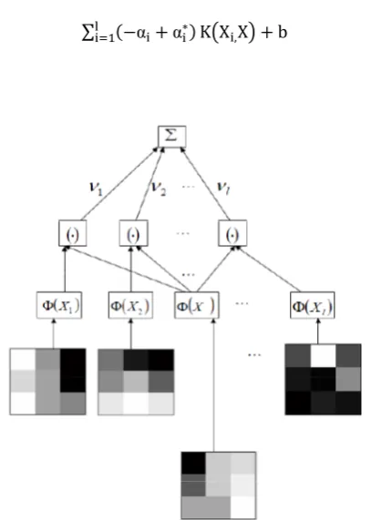
∑ (−α +α∗) K X
,X + b (5)
Fig. 1: Architecture of a regression machine constructed by the SV algorithm, vi = −αi +αi* b is added to the sum.
Fig. 1 shows the architecture of a regression machine constructed by the SV algorithm. It is similar to neural network regression. The difference is that the input layer in SVR are a subset of the training patterns (support vectors) and the test pattern. Fig. 2 shows the architecture of a traditional linear regression where the input layer is the test pattern alone. The complexity of SVR is O(nl), where n is the number of pixels in the input image and l is the number of SVs. The complexity of traditional linear regression is O(nm), where m is the number of coefficients (the size of the patch). In the example shown in Fig. 2, m is 9. SVR has much higher complexity since l ≫ m. Another difference is that SVR is adaptive while traditional regression is fixed.
As in Fig.2, (−αi + αi*) can be interpreted as the “weight” for each Xi and K (Xi , X ) can be viewed as the contribution of each SV. Though the weight is fixed, the contribution of each SV is adaptive to the input pattern X . When X is closer to a SV, that is, when the SV is a good example for the input pattern, then that SV contributes more to the final output. On the other hand, if a SV is different from X , then that SV has less influence in determining the output as K(Xi,X) will be small. Effectively, the kernel function K(Xi,X) measures the distance between a test pattern and the support vector [8].
Fig. 2: Linear regression diagram. The intercept b is added to the sum.
In this approach xp comes from the initial estimation of the LR image and yp is from the corresponding HR image. Where xp is the feature vector and yp is the corresponding observation. Then a model is learned by SVR. In the prediction process, the learned model will be applied to the input LR image to generate a super-resolved HR image.
III. SUPER-RESOLUTION
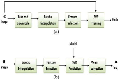
The algorithm consists of two processes: training and prediction, as shown in Fig. 3.
(a)
(b)
Fig 3. (a) Training process (b) Prediction Process
In the training process, we first blur the HR images and then downscale them by a factor of 2 to create the LR images. An initial estimation of the HR image is carried out using bicubic interpolation with an upscaling factor of 2 on the generated LR image. For each pixel at location (i , j) in the upscaled image, we take a local image patch of size m * m centered at (i , j) . This image patch is then weighted by a matrix of the same size. This matrix is constructed from a 2-D Gaussian distribution that assigns largest weight to the pixel at (i , j) and smaller weight to the other pixels that are
further away from the center pixel in the local patch. The weighted image patch is then converted to a row vector:
x, = vec(W (R,I )) (6)
Where IBI is the bicubic interpolated image and WG(Ri,j,IBI) is the weighted local image patch taken at (i , j) by the patch extraction operator Ri,j . Function vec reshapes the
matrix into a row vector x i,j of length m2 .
The gradient of the bicubic interpolated image is calculated in both horizontal and vertical direction at each pixel.
gh(i, j) =
1
2 (I, − I,) + I , − I ,)
g (i, j) = (I , − I,) + I , − I, ) (7)
Ii,j is the pixel value at (i, j) . The horizontal gradient magnitude gh(i,j) and the vertical gradient magnitude gv(i,j) are concatenated to the row vector xi , j .
For each pixel in the initially interpolated image at (i, j) , xi,j is now a m2 + 2 dimensional feature vector. The corresponding observation yi,j is the pixel value at position (i, j) in the HR image. SVR is supplied with all the feature vectors constructed from the training dataset and their corresponding observations. The generated model is then saved for the future use.
In the prediction process, we first upscale the testing LR image also using bicubic interpolation by the same factor of 2. For each pixel in the interpolated image, the local image patch of the same size is taken and the image gradient in two directions is calculated to get the features vectors in the same manner as we do in the training process. Now the output image z is constructed. The last step is to correct the mean of z since the mean of the upscaled image should be preserved to be the same as that of the input LR image due to the unchanged image structures and contents in the upscaling process. The pixel value of the final output at (i , j) is:
z, = z, (8) where mLR is the mean pixel value of the LR image and mz is the mean pixel value of z .
IV. EXPERIMENTAL RESULT
For the implementation of SVR LibSVM [9] is used. We choose Gaussian function as the kernel function. The parameters in the SVR are selected by cross-validation (C =362 ,Ɛ=2 and the standard deviation σ =1in the Gaussian kernel function). The downscaling factor for the HR images and the corresponding upscaling factor for the LR images are both 2. For both training and testing we only consider the luminance component of the images.
All the images used in the training and testing processes are originally taken from the USC-SIPI Image Database [10]. Both peak signal-to-noise ratio (PSNR) and structural
similarity (SSIM) are used to measure the quality of the
super-resolved images compared to original HR images. PSNR between two images of size M ×N is calculated by
PSNR = 10 log ∑ ∑∑ ∑( ( , ) ( , ) (9)
where 255 is the maximum possible gray pixel intensity value, x(i, j) and y(i, j) are the pixel values at the same location (i, j) from image x and y .
SSIM is designed to better match the human perception compared to PSNR, which sometimes is inconsistent with the visual observation . SSIM [11] defined as:
SSIM = µ µ σ
µ µ σ σ (10)
where x and y are the two images to be compared, µ and σ
are respectively the average and variance of the pixel values of the images x or y . σxy is the covariance of x and y. The value of SSIM is a scalar less than or equal to 1 and 1 means the two images in comparison are exactly the same.
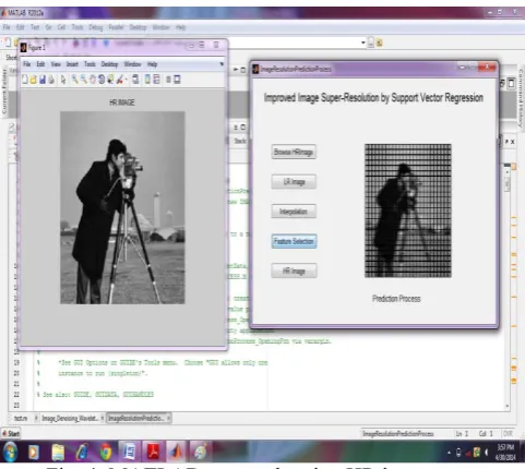
Fig. 4: MATLAB output showing HR image.
In this method feature selection is based on the pixel intensity values and gradient magnitude is comparing the result of the proposed method to the output of SVR with feature vectors that only contain the pixel values as similarly proposed method. It can be seen that by adding image gradient information to the feature vectors, the model learnt by SVR is capable of reconstructing edges and fine details from LR images. Final output HR image is shown in Fig.4.
The proposed super-resolution algorithm is compared with state-of-the-art methods including sparse coding SC[12] and kernel regression KR[13]. Also results by bicubic interpolation BI [4] are provided as reference.
Table I: MATLAB PSNR Result
Image BI [4] [12] SC [13] KR method Our
Cameraman 33.07 32.80 32.71 33.119 Elaine 35.24 34.55 33.72 39.394 House 34.57 33.80 33.71 36.006 Boat 32.49 32.33 31.72 33.318
Girl 36.26 36.21 35.34 37.855 Mandrill 30.89 31.00 30.35 31.013
Table II :MATLAB SSIM Result
Image BI [4] [12] SC [13] KR method Our Cameraman 0.818 0.835 0.756 0.8592
Elaine 0.921 0.916 0.860 0.9701 House 0.863 0.845 0.819 0.8562 Boat 0.799 0.838 0.707 0.8570
Girl 0.904 0.912 0.857 0.9615 Mandrill 0.648 0.738 0.551 0.8386
Table I and II show the PSNR and SSIM results for the test images in MATLAB. As shown, this method outperforms the other methods with respect to both PSNR and SSIM. Note that the reference methods are specifically designed for single image super-resolution.
The model learned by SVR in our method is able to generate fine details and sharp edges which lead to better visual quality. Both objective evaluation (by PSNR and SSIM) and subjective evaluation confirm the advantages of our method. By selecting more informative features besides pixel intensity and gradient, the result can be further improved. By adopting a larger and more comprehensive image dataset for training, the generated model would yield better results for image super resolution.
V. CONCLUSION
In this paper, an algorithm for single image super resolution based on support vector regression is implemented in MATLAB and compares the result with other state of art methods. In this paper we combining the pixel intensity values with local gradient information, the learned model by SVR from low-resolution image to high-resolution image is useful and robust for image super-resolution. The experiment is conducted on different types of images. Furthermore, the size of the training set is limited which makes the training relatively fast while still achieving good results. By comparing our method to the previous works, we find out that our method is able to produce better super-resolved images than state-of-the-art approaches. We believe that by selecting more informative features besides pixel intensity and gradient, the result can be further improved. By adopting a larger and more comprehensive image dataset for training, the generated model would yield better results for image super resolution.
ACKNOWLEDGMENT
I would like to convey my thanks to my project guide Mr. Anand M.J, for his valuable guidance, constant support and suggestions for improvement. I am also thankful to my parents and all teaching, non teaching staffs of PESCE, Mandya.
REFERENCES
[1] Le An and Bir Bhanu “Improved Image Super resolution by support vector regression” in Proc on Neural Networks , USA, 2011. [2] R. S. Wagner, D. E. Waagen, and M. L. Cassabaum, “Image
superresolution for improved automatic target recognition,” in Proc. SPIE, 2004, vol. 5426, pp. 188–196.
[3] R. Tsai, T. Huang, “Multi-frame image restoration and registration,” Advances in Computer Vision and Image Processing, vol. 1, no. 2, JAI Press Inc., Greenwich, CT, 1984, pp. 317–339.
[4] R. Keys, “Cubic convolution interpolation for digital image processing,” IEEE Transactions on Acoustics, Speech and Signal Processing, vol. 29, no. 6, pp. 1153-1160, 1981.
[5] J. Sun, Z. Xu, and H.-Y. Shum, “Image super-resolution using gradient profile prior,” In Proc. of the IEEE International Conference on Computer Vision and Pattern Recognition, pp. 1-8, 2008. [6] K. Ni, S. Kumar, N. Vasconcelos, and T. Q. Nguyen, "Single image
superresolution based on support vector regression", In Proc. of the IEEE International Conference on Acoustics, Speech and Signal Processing, pp. 601-604, 2006.
[7] D. Li, S. Simske, and R. Mersereau, “Single image super-resolution based on support vector regression”,
[8] A. J. Smola, and B. Schölkopf, “A tutorial on support vector regression,” Statistics and Computing 14, pp. 199–222, 2004. [9] C. -C. Chang, and C. -J. Lin, “LIBSVM: a library for support vector
machines,” 2001. Software available at:http://www.csie.ntu.edu.tw/~cjlin/libsvm
[10] Available at: http://sipi.usc.edu/database/
[11] Z. Wang, A. C. Bovik, H. R. Sheikh, and E. P. Simoncelli, “Image quality assessment: From error visibility to structural similarity,”IEEE Transactions on Image Processing, vol. 13, no. 4, pp. 600-612,2004.
[12] J. Yang, J. Wright, T. Huang, and Y. Ma. “Image Super-resolution as Sparse Representation of Raw Image Patches,” In Proc. of the IEEE International Conference on Computer Vision and Pattern Recognition, pp. 1-8, 2008.
[13] H. Takeda, S. Farsiu, and P. Milanfar, “Kernel regression for image processing and reconstruction,” IEEE Transactions on Image Processing, vol. 16, no. 4, pp. 349-366, 2007
AUTHORS
Sowmya.M received Bachelor of engineering in Electronics and communication from ‘VidyaVikas College of Engineering’, Mysore in 2012. She is currently pursuing her M.Tech degree in VLSI and Embedded Systems at PESCE College of Engineering, Mandya , under ‘Visvesvaraya Technological University’, Belgaum.
Anand M.J. received B.E in Instrumentation Technology from ‘Sri Jayachamarajendra College of Engineering’, under ‘University Of Mysore’ in Mysore. And he received M.Tech degree in VLSI and Embedded Systems at Sri Jayachamarajendra College of Engineering under ‘Visvesvaraya Technological University’, Belgaum.Currently he is working as Assistant Professor in PESCE College of Engineering, Mandya.