Daniel J. Bernstein1,2, Chitchanok Chuengsatiansup1, David Kohel3, and Tanja Lange1
1 Department of Mathematics and Computer Science
Technische Universiteit Eindhoven
P.O. Box 513, 5600 MB Eindhoven, The Netherlands [email protected], [email protected]
2
Department of Computer Science University of Illinois at Chicago
Chicago, IL 60607–7045, USA [email protected]
3 Institut de Math´ematiques de Marseille
Aix-Marseille Universit´e 163, avenue de Luminy, Case 907 13288 Marseille CEDEX 09, France
Abstract. This paper presents new speed records for arithmetic on a large family of elliptic curves with cofactor 3: specifically, 8.77Mper bit for 256-bit variable-base single-scalar multiplication when curve param-eters are chosen properly. This is faster than the best results known for cofactor 1, showing for the first time that points of order 3 are useful for performance and narrowing the gap to the speeds of curves with cofactor 4.
Keywords:efficiency, elliptic-curve arithmetic, double-base chains, fast arithmetic, Hessian curves, complete addition laws
1
Introduction
performance/security tradeoff for elliptic-curve cryptography. All of the latest speed records for ECC are set by curves with cofactor divisible by 2, with base fields Fq where q is a square, and with extra endomorphisms: Faz-Hern´andez– Longa–S´anchez [27] use a twisted Edwards GLS curve with cofactor 8 over Fq where q = (2127 −5997)2; Oliveira–L´opez–Aranha–Rodr´ıguez-Henr´ıquez [49] use a GLV+GLS curve with cofactor 2 over Fq where q = 2254; and Costello– Hisil–Smith [20] use a Montgomery Q-curve with cofactor 4 (and twist cofactor 8) over Fq where q = (2127 −1)2. Similarly, for “conservative” ECC over prime fields without extra endomorphisms, Bernstein [5] uses a Montgomery curve with cofactor 8 (and twist cofactor 4), and Bernstein–Duif–Lange–Schwabe–Yang [7] use an equivalent twisted Edwards curve.
The very fast Montgomery ladder for Montgomery curves [42] was published at the dawn of ECC, and its speed always relied on a cofactor divisible by 4. However, for many years the benefit of such cofactors seemed limited to ladders for variable-base single-scalar multiplication. Cofactor 1 seemed slightly faster than cofactor 4 for signature generation and signature verification; NIST’s curves were published in the context of a signature standard. Many years of investiga-tions of addition formulas for a wide range of curve shapes (see, e.g., [17], [19], [34], [41], and [13]) failed to produce stronger arguments for cofactors above 1 — until the advent [24] and performance analysis [9] of Edwards curves.
Cofactor 3. Several papers have tried to exploit a different cofactor, namely 3,
as follows. Hessian curvesx3+y3+ 1 =dxy, which always have points of order 3 over finite fields, have a very simple and symmetric addition law due to Sylvester. Chudnovsky–Chudnovsky in [17] already observed that this law requires just 12M in projective coordinates. However, Hessian doublings were much slower than Jacobian-coordinate Weierstrass doublings, and this slowdown outweighed the addition speedup, since (in most applications) doublings are much more frequent than additions. The best way to handle a curve with cofactor 3 was to forget about the points of order 3 and simply use the same formulas used for curves with cofactor 1.
What we show in this paper, for the first time, is how to use cofactor 3 to beat the best available results for cofactor 1. We do not claim to have beaten cofactor 4, but we have significantly narrowed the gap.
We now review previous speeds and compare them to our speeds. We adopt the following rules to maximize comparability:
– For individual elliptic-curve operations we count multiplications and squar-ings. M is the cost of a multiplication, and S is the cost of a squaring. We do not count additions or subtractions. (Computer-verified operation counts for our formulas, including counts of additions and subtractions, appear in the latest update of EFD [8].)
– We also count multiplications by curve parameters: e.g., Md is the cost of multiplying by d. We assume that curves are sensibly chosen with small d. In summaries we take Md = 0.
– We do not include the cost of final conversion to affine coordinates. We also assume that inversion is not fast enough to make intermediate inversions useful. Consequently the exact cost of inversion does not appear.
– We focus on the traditional case of variable-base single-scalar multiplication, in particular for average 256-bit scalars. Beware that this is only loosely correlated with other scalar-multiplication tasks. (Other tasks tend to rely more on additions, so the fast complete addition law for twisted Hessian curves should provide an even larger benefit compared to Weierstrass curves.) Bernstein–Lange in [10] analyzed scalar-multiplication performance on several curve shapes and concluded, under these assumptions, that Weierstrass curves y2 =x3 −3x+a6 in Jacobian coordinates used 9.34M per bit on average, and that Hessian curves were slower. Bernstein–Birkner–Lange–Peters in [6] used double-base chains (doublings, triplings, and additions) to considerably speed up Hessian curves to 9.65Mper bit and to slightly speed up Weierstrass curves to 9.29M per bit. Hisil in [32, Table 6.4], without double-base chains, reported more than 10Mper bit for Hessian curves.
Our new results are just 8.77M per bit. This means that one actually gains something by taking advantage of a point of order 3. The new speeds require a base field with 66= 0 and with fast multiplication by a primitive cube root of 1, such as a field of the formFp[ω]/(ω2+ω+ 1) where p∈2 + 3Z. This quadratic field structure might seem to constrain the applicability of the results, but (1) GLS-curve and Q-curve results already show that a quadratic field structure is desirable for performance; (2) there is also a fast primitive cube root of 1 in, e.g., the prime field Fp where 7p = 2298 + 2149 + 1; (3) we do not lose much speed from more general fields (the cost of a tripling increases by 0.4M). Note that the 8.77Mper bit does not use the speedups in (1). Our speedups can be combined with the speedups in (1) but we have not quantified the resulting performance.
Completeness, side channels, and precomputation. For a large fraction
of curves, the formulas we use have a further benefit not reflected in the mul-tiplication counts stated above: namely, the formulas are complete. This means that the formulas work for all curve points. The implementor does not have to waste any time checking for exceptional cases, and does not have to worry that an attacker can generate inputs that trigger exceptional cases: there are no ex-ceptional cases. (For comparison, a strongly unified but incomplete addition law works for most additions and works for most doublings, but still has exceptional cases. The traditional addition law for Weierstrass curves is not even strongly unified: it consistently fails for doublings.)
crypto-graphic protocols, such as signature verification, and also in many other elliptic-curve computations, such as the elliptic-elliptic-curve method of integer factorization.
We also allow scalar-multiplication techniques that rely on scalar-dependent precomputation. This is reasonable for applications that reuse a single scalar many times. For example, in the context of signatures, the signer can carry out the precomputation and compress the results into the signature. The signer can also choose different techniques for different scalars: in particular, there are some scalars where our cofactor-3 techniques are even faster than cofactor 4. One can easily find, and we suggest choosing, curves of cofactor 12 that simul-taneously allow the current cofactor-3 and cofactor-4 methods; these curves are also likely to be able to take advantage of any future improvements in cofactor-3 and cofactor-4 methods.
Tools and techniques. At a high level, we use a tree search for double-base
chains, allowing windows and taking account of the costs of doublings, triplings, and additions. At a lower level, we use tripling formulas that take 6M+ 6S, doubling formulas that take 6M+ 2S, and addition formulas that take 11M; in this overview we ignore multiplications by constants. These formulas work in projective coordinates for Hessian curves.
Completeness relies on two further tools. First, we use a rotated addition law. Unlike the standard (Sylvester) addition law, the rotated addition law is strongly unified. In fact, the rotated addition law works in every case where the standard addition law fails; i.e., the two laws together form a complete system of addition laws. Second, we work more generally with twisted Hessian curves ax3+y3 + 1 = dxy. If a is not a cube then the rotated addition law by itself is complete. The doubling formulas and tripling formulas are also complete, meaning that they have no exceptional cases. The generalization also provides more flexibility in finding curves with small parameters.
For comparison, Jacobian coordinates for Weierstrass curvesy2 =x3−3x+a6 use 7M+ 7S for tripling, 3M+ 5S for doubling, and 11M+ 5Sfor addition. This saves 3(M−S) in doubling but loses M+S in tripling and loses 5S in addition. Given these operation counts it is not a surprise that we beat Weierstrass curves. 6M + 6S triplings were achieved once before, namely by tripling-oriented Doche–Icart–Kohel curves [22]. Those curves also offer 2M+ 7Sdoublings, com-petitive with our 6M+ 2S. However, the best addition formulas known for those curves take 11M+ 6S, even slower than Weierstrass curves.
As noted earlier, Edwards curves are still faster for average scalars, thanks to their particularly fast doublings and additions. However, we do beat Edwards curves for scalars that involve many triplings.
Credits and priority dates.Hessian curves and the standard addition law are
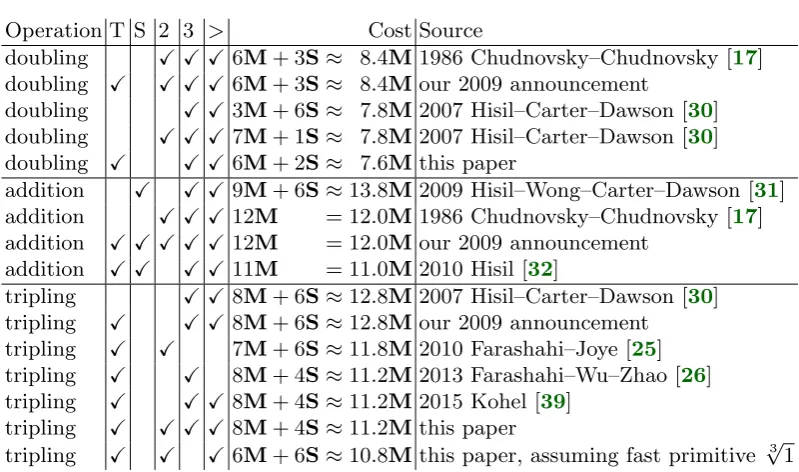
Operation T S 2 3 > Cost Source
doubling X X X6M+ 3S≈ 8.4M 1986 Chudnovsky–Chudnovsky [17] doubling X X X X6M+ 3S≈ 8.4M our 2009 announcement
doubling X X3M+ 6S≈ 7.8M 2007 Hisil–Carter–Dawson [30] doubling X X X7M+ 1S≈ 7.8M 2007 Hisil–Carter–Dawson [30] doubling X X X6M+ 2S≈ 7.6M this paper
addition X X X9M+ 6S≈13.8M 2009 Hisil–Wong–Carter–Dawson [31] addition X X X12M = 12.0M 1986 Chudnovsky–Chudnovsky [17] addition X X X X X12M = 12.0M our 2009 announcement
addition X X X X11M = 11.0M 2010 Hisil [32]
tripling X X8M+ 6S≈12.8M 2007 Hisil–Carter–Dawson [30] tripling X X X8M+ 6S≈12.8M our 2009 announcement
tripling X X 7M+ 6S≈11.8M 2010 Farashahi–Joye [25] tripling X X 8M+ 4S≈11.2M 2013 Farashahi–Wu–Zhao [26] tripling X X X8M+ 4S≈11.2M 2015 Kohel [39]
tripling X X X X8M+ 4S≈11.2M this paper
tripling X X X6M+ 6S≈10.8M this paper, assuming fast primitive √31 Table 1.1. Costs of various formulas for Hessian curves in projective coordinates. Costs are sorted using the assumption S ≈ 0.8M; note that S/M is normally much smaller in characteristic 2. “T” means that the formula was stated for twisted Hessian curves, not just Hessian curves; all of the “T” formulas are complete for suitable curves. “S” means “strongly unified”: an addition formula that also works for doubling. “2” means that the formula works in characteristic 2. “3” means that the formula works in characteristic 3. “>” means that the formula works in characteristic above 3.
the completeness result in [4, page 40], and contributing a “twisted Hessian” section to EFD), but this paper is our first formal publication of these results.
The speeds that we announced at that time for twisted Hessian curves were no better than known speeds for standard formulas for Hessian curves: 8M+ 6S
for tripling, 6M+ 3S for doubling, and 12Mfor addition. Followup work found better formulas for all of these operations. Almost all of those formulas are superseded by formulas that we now announce; the only exception is that we use 11Maddition formulas [32] from Hisil. See Table 1.1 for an overview.
Tripling: One of the followup papers [25], by Farashahi–Joye, reported 7M+ 6S for twisted Hessian tripling, but only for characteristic 2. Another followup paper [26], by Farashahi–Wu–Zhao, reported 4 multiplications and 4 cubings, overall 8M+ 4S, for Hessian tripling, but only for characteristic 3. Further fol-lowup work [39], by Kohel, reported 4 multiplications and 4 cubings for twisted Hessian tripling in any odd characteristic. In Section 6 we generalize the approach of [39] and show how a better specialization reduces cost to just 6 cubings, as-suming that the field has a fast primitive cube root of 1.
introduced doubling formulas using 3M+ 6S, and also introduced doubling for-mulas using 7M+ 1S, using techniques that seem to be specific to small cube a such asa = 1; see also [32]. Our 6M+ 2S is better than 7M+ 1S if S <M, and is better than 3M+ 6S if S >0.75M.
At a higher level, double-base chains have been explored in several papers. The idea of a tree search for double-base chains was introduced by Doche and Habsieger in [21]. The tree search in [21] tries to minimize the number of addi-tions used in a double-base chain, ignoring the cost of doublings and triplings; we do better by using the cost of doublings and triplings to adjust the weights of nodes in the tree.
2
Twisted Hessian curves
Definition 2.0. Let k be a field. A projective twisted Hessian curve over
k is a curve of the form aX3 +Y3 +Z3 = dXY Z in P2 with specified point (0 :−1 : 1), where a, d are elements of k with a(27a−d3)6= 0.
Theorem 2.1 below states that any projective twisted Hessian curve is an elliptic curve. The correponding affine curve ax3+y3+ 1 =dxy with specified point (0,−1) is anaffine twisted Hessian curve.
We state theorems for the projective curve, and allow the reader to deduce corresponding theorems for the affine curve. When we say “LetH be the twisted Hessian curve aX3+Y3+Z3 =dXY Z over k” we mean that a, dare elements of k, that a(27a−d3) 6= 0, and that H is the projective twisted Hessian curve aX3+Y3+Z3 =dXY Z inP2 with specified point (0 :−1 : 1). Some theorems need, and state, further assumptions such as d 6= 0.
The special casea = 1 of a twisted Hessian curve is simply aHessian curve. The twisted Hessian curveaX3+Y3+Z3 =dXY Z is isomorphic to the Hessian curve ¯X3+Y3+Z3 = (d/a1/3) ¯XY Z over any extension ofk containing a cube root a1/3 of a: simply take ¯X = a1/3X. Similarly, taking ¯X = dX when d 6= 0 shows that the twisted Hessian curve for (a, d) is isomorphic to the twisted Hessian curve for (a/d3,1); but we retain a and d as separate parameters to allow more curves with small parameters and thus with fast arithmetic.
Hessian curves have a long history, but twisted Hessian curves do not. The importance of twisted Hessian curves, beyond their extra generality, is that they have a complete addition law when a is not a cube. See Theorem 4.5 below.
Proof strategy: twisted Hessian curves as foundations. One can use the
We do not claim that this tracking involves any particular difficulty. In one case the tracking has been done before: specifically, some of the nonsingularity computations in Theorem 2.1 are special cases of classical discriminant compu-tations for ternary cubics aX3 +bY3 +cZ3 = dXY Z. See, e.g., [2] and [16]. However, the classical computations were carried out in characteristic 0, and the range of validity of the computations is not always obvious. Many of the compu-tations fail in characteristic 3, even though Theorem 2.1 is valid in characteristic 3. Since the complete proofs are straightforward we simply include them here.
Similarly, one can derive many features of twisted Hessian curves from corre-sponding well-known features of Weierstrass curves, but we instead give direct proofs. We do use Weierstrass curves inside Theorem 5.2, which proves a prop-erty of all elliptic curves having points of order 3.
Notes on definitions: Hessian curves. There are various superficial
dif-ferences among the definitions of Hessian curves in the literature. First, often characteristic 3 is prohibited. For example, [50] considers only base fields Fq withq ∈2 + 3Z, and [34] considers only characteristics larger than 3. Our main interest is in the case q ∈ 1 + 3Z, and in any event we see no reason to restrict the characteristic in the definition.
Second, often constants are introduced into the parameter d. For example, [34] defines a Hessian curve asX3+Y3+Z3 = 3dXY Z, and the curve actually considered by Hesse in [29, page 90, formula 54] wasX3+Y3+Z3+6dXY Z = 0. Third, the specified point is often taken as a point at infinity, specifically (−1 : 1 : 0); see, e.g., [17]. We use an affine point (0 :−1 : 1) to allow completeness of theaffinetwisted Hessian curve rather than merely completeness of theprojective twisted Hessian curve; if a is not a cube then there are no points at infinity for implementors to worry about. Converting addition laws (and twists and so on) between these two choices of neutral element is a trivial matter of permuting X, Y, Z.
Notes on definitions: elliptic curves. There are also various differences
among the definitions of elliptic curves in the literature.
The most specific definitions would say that Hessian curves are not elliptic curves: for example, Koblitz in [36, page 117] defines elliptic curves to have long Weierstrass form. Obviously we do not use such restrictive definitions.
Two classical definitions that allow Hessian curves are as follows: (1) an el-liptic curve is a nonsingular cubic curve in P2 with a specified point; (2) an elliptic curve is a nonsingular cubic curve inP2 with a specified inflection point. The importance of the inflection-point condition is that it allows the traditional geometric addition law: three distinct curve points on a line have sum 0; more generally, all curve points on a line, counted with multiplicity, have sum 0. If the specified point were not an inflection point then the addition law would be more complicated. See, e.g., [33, Chapter 3, Theorem 1.2].
These definitions are still not broad enough to allow, e.g., Edwards curves as elliptic curves. Edwards curves in P2 are singular and not cubic; the Ar`ene– Lange–Naehrig–Ritzenthaler geometric addition law [1] for Edwards curves is not the traditional geometric addition law; etc. “Elliptic curve” is often defined more broadly as “smooth projective genus-1 curve with a specified point”, but this leaves ambiguous whether a “projective curve” is a curve for which there exists an embedding into projective space or a curveequipped with an embedding into projective space. With the first notion, the concept of addition laws for a curve is ill-defined, as is any other concept that relies on choices of coordinates. The second notion does not admit, e.g., Edwards curves in P1 ×P1 as elliptic curves; it does allow Edwards curves in P3, but the switch from P1×P1 to P3
damages the performance of doublings, so this definition is not broad enough for a serious analysis of performance. We avoid further discussion of ways to define elliptic curves in more generality: all of our theorems are focused on twisted Hessian curves, and then the classical definitions suffice.
Theorem 2.1. Let H be the twisted Hessian curve aX3 +Y3 +Z3 = dXY Z
over a field k. Then H is an elliptic curve.
Proof. aX3 +Y3 +Z3 = dXY Z is a cubic curve in P2, and (0 : −1 : 1) is a point on the curve. What remains is to prove that this curve is nonsingular.
Recall thata(27a−d3)6= 0 by definition of twisted Hessian curves.
A singularity (X : Y : Z) ∈ P2 of aX3 + Y3 + Z3 = dXY Z satisfies 3aX2 =dY Z, 3Y2 =dXZ, and 3Z2 = dXY. We will deduce X =Y =Z = 0, contradicting (X :Y :Z)∈P2.
Case 1: 36= 0 in k. Multiply to obtain 27aX2Y2Z2 =d3X2Y2Z2, i.e., (27a− d3)X2Y2Z2 = 0. By hypothesis 27a−d3 6= 0, so X2Y2Z2 = 0, so X = 0 or Y = 0 or Z = 0.
Case 1.1:X = 0. Then 3Y2 = 0 and 3Z2 = 0 so Y = 0 and Z = 0 as claimed. Case 1.2: Y = 0. Then 3aX2 = 0 and 3Z2 = 0, and a 6= 0 by hypothesis, so X = 0 and Z = 0 as claimed.
Case 1.3: Z = 0. Then 3aX2 = 0 and 3Y2 = 0, and again a 6= 0, so X = 0 and Y = 0 as claimed.
Case 2: 3 = 0 ink. Then dY Z = 0 anddXZ = 0 anddXY = 0. By hypothesis a(−d3)6= 0, so d6= 0, so at least two of the coordinates X, Y, Z are 0.
Case 2.1: X = Y = 0. Then the curve equation aX3 +Y3 +Z3 = dXY Z forces Z3 = 0 so Z = 0 as claimed.
Case 2.2: X = Z = 0. Then the curve equation forces Y3 = 0 so Y = 0 as claimed.
Case 2.3:Y =Z = 0. Then the curve equation forces aX3 = 0, and a 6= 0 by
hypothesis, so X = 0 as claimed. ut
Theorem 2.2. Let H be the twisted Hessian curve aX3 +Y3 +Z3 = dXY Z
over a field k. Then (0 :−1 : 1) is an inflection point on H.
k. Consequently, by B´ezout’s theorem, this point has intersection multiplicity 3. (An alternative proof, involving essentially the same calculation, computes the multiplicity directly from its definition.)
To prove the claim, assume that−3(Y+Z) =dX andaX3+Y3+Z3 =dXY Z. Then (27a−d3)X3 = 27aX3−(−3(Y +Z))3 = 27(aX3+ (Y +Z)3) = 27(aX3+ Y3+Z3+ 3(Y +Z)Y Z) = 27(dXY Z−dXY Z) = 0 so X3 = 0 so X = 0. Now Y +Z = 0: this follows from −3(Y +Z) =dX = 0 if 3 6= 0 in k, and it follows from Y3+Z3 = 0 if 3 = 0 in k. Thus (X :Y :Z) = (0 :−1 : 1). ut
3
The standard addition law
Theorem 3.2 states an addition law for twisted Hessian curves. We originally derived this addition law as follows:
– Start from Sylvester’s addition law for X3+Y3 +Z3 = dXY Z. See, e.g., [17, page 425, equation 4.21i].
– Observe, as noted in [17], that the addition law is independent ofd.
– Conclude that the addition law also works for X3+Y3 +Z3 = (d/c)XY Z, where c is a cube root of a.
– Permute X, Y, Z to our choice of neutral element.
– Replace X withcX.
– Rescale the outputs X3, Y3, Z3 by a factor c.
The resulting polynomials X3, Y3, Z3 are identical to Sylvester’s addition law: they are independent of curve parameters, and in particular are independent of a. We refer to this addition law as the standard addition law. For reasons explained in Section 2, we prove Theorem 3.2 here by giving a direct proof of the standard addition law for the general case, rather than deriving the general case from the special casea = 1.
The standard addition law is never complete: it fails whenever (X2 :Y2 :Z2) = (X1 :Y1 :Z1). More generally, it fails if and only if (X2 :Y2 :Z2)−(X1 :Y1 :Z1) has the form (0 :−ω : 1) where ω3 = 1, or equivalently (X2 :Y2 :Z2) = (ω2X1 : ωY1 :Z1). See Theorem 4.6 for the equivalence, and Theorem 3.3 for the failure analysis.
A different way to analyze the failure cases, with somewhat less calculation, is as follows. First prove that (X2 :Y2 :Z2) has the form (0 :−ω : 1) if and only if the addition law fails to add the neutral element (0 :−1 : 1) to (X2 :Y2 :Z2). Then use a theorem of Bosma and Lenstra [14, Theorem 2] stating that the set of failure cases of a degree-(2,2) addition law for a cubic elliptic curve inP2 is a union of shifted diagonals∆S ={(P1, P1+S)}. The theorems in [14] are stated only for Weierstrass curves, but they are invariant under linear equivalence and thus also apply to twisted Hessian curves. See [38] for a generalization to elliptic curves embedded in projective space of any dimension.
Theorem 3.1. Let H be the twisted Hessian curve aX3 +Y3 +Z3 = dXY Z over a field k. Let X1, Y1, Z1 be elements of k such that (X1 :Y1 :Z1) ∈ H(k). Then −(X1 :Y1 :Z1) = (X1 :Z1 :Y1).
Proof. Recall that the specified neutral element of the curve is (0 :−1 : 1). Case 1: (X1 : Y1 : Z1) 6= (X1 : Z1 : Y1). Then X1(Y +Z) = X(Y1 +Z1) is a line in P2: if all its coefficients −Y1−Z1, X1, X1 are 0 then (X1 :Y1 :Z1) = (0 : −1 : 1) = (X1 : Z1 : Y1), contradiction. This line intersects the curve at the distinct points (0 : −1 : 1), (X1 : Y1 : Z1), and (X1 : Z1 : Y1). Hence −(X1 :Y1 :Z1) = (X1 :Z1 :Y1).
Case 2: (X1 : Y1 : Z1) = (X1 :Z1 : Y1) and X1 6= 0. Again (X1 : Y1 : Z1)6= (0 : −1 : 1), and again X1(Y +Z) = X(Y1 +Z1) is a line. This line intersects the curve at both (0 :−1 : 1) and (X1 :Y1 :Z1), and we show in a moment that it is the tangent to the curve at (X1 :Y1 : Z1). Hence −(X1 : Y1 : Z1) = (X1 : Y1 :Z1) = (X1 :Z1 :Y1).
For the tangent calculation we take coordinates y=Y /X and z =Z/X. The curve is thena+y3+z3 =dyz; the pointP1 is (y1, z1) = (Y1/X1, Z1/X1), which by hypothesis satisfies y1 = z1; and the line is y+z = y1 +z1. The curve is symmetric betweeny and z, so its slope at (y1, z1) = (z1, y1) must be−1, which is the same as the slope of the line.
Case 3: (X1 :Y1 :Z1) = (X1 :Z1 :Y1) and X1 = 0. Then Y13+Z13 = 0 by the curve equation so Y1 =λZ1 for some λ with λ3 =−1; but (Y1 :Z1) = (Z1 :Y1) implies λ = 1/λ, so λ = −1, so (X1 : Y1 :Z1) = (0 :−1 : 1). Hence −(X1 :Y1 : Z1) = (0 :−1 : 1) = (0 : 1 :−1) = (X1 :Z1 :Y1). ut
Theorem 3.2. Let H be the twisted Hessian curve aX3 +Y3 +Z3 = dXY Z
over a field k. Let X1, Y1, Z1, X2, Y2, Z2 be elements of k such that (X1 : Y1 : Z1),(X2 :Y2 :Z2)∈H(k). Define
X3 =X12Y2Z2−X22Y1Z1, Y3 =Z12X2Y2−Z22X1Y1, Z3 =Y12X2Z2−Y22X1Z1.
If (X3, Y3, Z3)6= (0,0,0) then (X1 :Y1 :Z1) + (X2 :Y2 :Z2) = (X3 :Y3 :Z3). Proof. The polynomial identity
aX33+Y33+Z33 −dX3Y3Z3
= (X13Y23Z23+Y13X23Z23+Z13X23Y23−3X1Y1Z1X22Y 2 2Z
2 2)(aX
3 1+Y
3 1+Z
3
1−dX1Y1Z1) −(X23Y13Z13+Y23X13Z13+Z23X13Y13−3X2Y2Z2X12Y12Z12)(aX23+Y23+Z23−dX2Y2Z2) implies that (X3 : Y3 : Z3) ∈ H(k). The rest of the proof uses the chord-and-tangent definition of addition to show that (X1 : Y1 : Z1) + (X2 : Y2 : Z2) = (X3 :Y3 :Z3).
The line through (X1 : Y1 : Z1) and (X2 : Y2 : Z2) is (Z1Y2 −Z2Y1)X + (X1Z2−X2Z1)Y + (X2Y1−X1Y2)Z = 0. The polynomial identity
(Z1Y2−Z2Y1)X3+ (X1Z2−X2Z1)Z3+ (X2Y1−X1Y2)Y3 = 0 shows that (X3 :Z3 :Y3) is also on this line.
One would now like to conclude that (X1 :Y1 :Z1) + (X2 :Y2 :Z2) =−(X3 : Z3 : Y3), so (X1 : Y1 : Z1) + (X2 : Y2 : Z2) = (X3 : Y3 : Z3) by Theorem 3.1. The only difficulty is that (X3 :Z3 :Y3) might be the same as (X1 :Y1 :Z1) or (X2 :Y2 :Z2); the rest of the proof consists of verifying that, in these two cases, the line is the tangent to the curve at (X3 :Z3 :Y3).
We use two other easy polynomial identities. First, X1Y2Y3 + Y1Z2X3 + Z1X2Z3 = 0. Second,aX1X2X3+Z1Z2Y3+Y1Y2Z3 = (aX13+Y13+Z13)X2Y2Z2− (aX23+Y23+Z23)X1Y1Z1. The curve equations for (X1 : Y1 :Z1) and (X2 :Y2 : Z2) then imply aX1X2X3+Z1Z2Y3+Y1Y2Z3 = 0.
Case 1: (X3 :Z3 : Y3) = (X1 :Y1 : Z1). The two identities above then imply X1Y2Z1 +Y1Z2X1+Z1X2Y1 = 0 and aX12X2 +Z12Z2 +Y12Y2 = 0 respectively. Our line is (Z1Y2−Z2Y1)X+ (X1Z2−X2Z1)Y + (X2Y1−X1Y2)Z = 0, while the tangent to the curve at (X1 :Y1 :Z1) is (3aX12−dY1Z1)X+ (3Y12−dX1Z1)Y + (3Z12−dX1Y1)Z = 0. To see that these lines are the same, observe that the cross product
(3Y2
1 −dX1Z1)(X2Y1−X1Y2)−(3Z12−dX1Y1)(X1Z2−X2Z1) (3Z12−dX1Y1)(Z1Y2−Z2Y1)−(3aX12−dY1Z1)(X2Y1−X1Y2) (3aX12−dY1Z1)(X1Z2−X2Z1)−(3Y12−dX1Z1)(Z1Y2−Z2Y1)
is exactly
3X2 −3X1 dX1 3Y2 −3Y1 dY1 3Z2 −3Z1 dZ1
aX3
1 +Y13+Z13−dX1Y1Z1 aX12X2+Z12Z2+Y12Y2 X1Y2Z1+Y1Z2X1+Z1X2Y1
=
0 0 0
.
Case 2: (X3 : Z3 : Y3) = (X2 : Y2 : Z2). Exchanging (X1 : Y1 : Z1) with (X2 : Y2 : Z2) replaces (X3, Y3, Z3) with (−X3,−Y3,−Z3) and moves to case
1. ut
Theorem 3.3. In the situation of Theorem 3.2, (X3, Y3, Z3) = (0,0,0) if and
only if (X2 :Y2 :Z2) = (ω2X1 :ωY1 :Z1) for some ω∈k with ω3 = 1.
Proof. If (X2 : Y2 : Z2) = (ω2X1 : ωY1 : Z1) and ω3 = 1 then (X3, Y3, Z3) is proportional to (X2
1ωY1Z1−ω4X12Y1Z1, Z12ω2X1ωY1−Z12X1Y1, Y12ω2X1Z1− ω2Y12X1Z1) = (0,0,0).
Conversely, assume that (X3, Y3, Z3) = (0,0,0). Then X12Y2Z2 = X22Y1Z1, Z12X2Y2 =Z22X1Y1, andY12X2Z2 =Y22X1Z1.
ω =λ2/λ1; then ω3 = λ32/λ13 = 1 and (X2 : Y2 : Z2) = (0 : λ2 : 1) = (0 : ωλ1 : 1) = (ω2X1 :ωY1 :Z1).
If X2 = 0 then similarly X1 = 0. Assume from now on that X1 6= 0 and X2 6= 0. Writey1 =Y1/X1, z1 =Z1/X1,y2 =Y2/X2, and z2 =Z2/X2. Rewrite the three equations X3 = 0, Y3 = 0, and Z3 = 0 as y2z2 = y1z1, z12y2 = z22y1, and y21z2 = y22z1. The first two equations imply z13y1 = z21y2z2 = z23y1, so (z13 −z32)y1 = 0; the first and third equations imply y13z1 = y12y2z2 = y23z1, so (y31−y23)z1 = 0.
If y1 = 0 then z12y2 = 0 by the second equation. The curve equation a+ y31 +z13 =dy1z1 forces a+z31 = 0 so z1 6= 0; hence y2 = 0. The curve equation a+y23+z32 =dy2z2 similarly forces a+z32 = 0 soz23 =z13. Write ω =z2/z1; then ω3 = 1 and (X2 : Y2 : Z2) = (1 : y2 : z2) = (1 : 0 : z2) = (1 : 0 : ωz1) = (ω2 : ωy1 :z1) = (ω2X1 :ωY1 :Z1).
If z1 = 0 then similar logic applies. Assume from now on that y1 6= 0 and z1 6= 0. Then z13 =z23 and y13 =y32. Write ω =y1/y2; then ω3 = 1. The equation X3 = 0 forces ω = z2/z1. Hence (X2 : Y2 : Z2) = (1 : y2 : z2) = (1 : ω−1y1 :
ωz1) = (ω2X1 :ωY1 :Z1). ut
4
The rotated addition law
Theorem 4.2 states a new addition law for twisted Hessian curves. This addition law is obtained as follows:
– Subtract (1 : −c : 0) from one input, using Theorem 4.1, where c is a cube root of a.
– Use the standard addition law in Theorem 3.2.
– Add (1 : −c: 0) to the output, using Theorem 4.1 again.
The formulas in Theorem 4.1 are linear, so the resulting addition law has the same bidegree as the standard addition law. This is an example of what Bernstein and Lange in [11, Section 8] call rotation of an addition law.
This rotated addition law is new, even in the case a = 1. Unlike the stan-dard addition law, the rotated addition law works for doublings. Specializing the rotated addition law to doublings, and further to a = 1, produces exactly the Joye–Quisquater doubling formula from [34, Proposition 2]. Even better, the rotated addition law is complete whena is not a cube; see Theorem 4.5 below.
Theorem 4.7 states that the standard addition law and the rotated addition law form a complete system of addition laws for any twisted Hessian curve: any pair of input points can be added by at least one of the two laws. This system is vastly simpler than the Bosma–Lenstra complete system [14] of addition laws for Weierstrass curves, and arguably even simpler than the Bernstein–Lange complete system [11] of addition laws for twisted Edwards curves: each output coordinate here is a difference of just two degree-(2,2) monomials, as in [11], but here there are just three output coordinates while in [11] there were four.
addition law. One can also prove that these three addition laws are a basis for the space of degree-(2,2) addition laws for H: it is easy to see that the laws are linearly independent, and Bosma and Lenstra showed in [14, Section 4] that the whole space has dimension 3.
Theorem 4.1. Let H be the twisted Hessian curve aX3 +Y3 +Z3 = dXY Z
over a field k. Assume that c ∈ k satisfies c3 = a. Then (1 : −c : 0) ∈ H(k). Furthermore, if X1, Y1, Z1 are elements of k such that (X1 : Y1 : Z1) ∈ H(k), then (X1 :Y1 :Z1) + (1 :−c: 0) = (Y1 :cZ1 :c2X1).
Proof. First a(1)3+ (−c)3+ (0)3 = 0 so (1 :−c: 0)∈H(k).
Case 1: Z1 6= 0. Write (X2, Y2, Z2) = (1,−c,0), and define (X3, Y3, Z3) as in Theorem 3.2. ThenX3 =−Y1Z1, Y3 =−cZ12, and Z3 =−c2X1Z1, so (X3 :Y3 : Z3) = (Y1 : cZ1 : c2X1), so (X1 : Y1 :Z1) + (1 : −c : 0) = (Y1 :cZ1 : c2X1) by Theorem 3.2.
Case 2: Z1 = 0. (Note that Theorem 3.2 is not useful in this case, since it defines (X3, Y3, Z3) = (0,0,0).) Then aX13 +Y13 = 0 by the curve equation, so X1 6= 0 and Y1 6= 0. Write ω = Y1/(−cX1); then ω3 = Y13/(−aX13) = 1, and (X1 :Y1 :Z1) = (1 :−ωc: 0).
Case 2.1: ω 6= 1. The line Z = 0 intersects the curve at the three distinct points (1 :−c: 0), (1 : −ωc: 0), and (1 :−ω−1c: 0), so (1 :−c: 0) + (1 : −ωc: 0) = −(1 :−ω−1c: 0) = (1 : 0 :−ω−1c) = (−ωc: 0 : c2) = (Y
1 : cZ1 : c2X1) by Theorem 3.1.
Case 2.2:ω = 1, i.e., (X1 :Y1 :Z1) = (1 :−c: 0). The line 3c2X+3cY+dZ= 0 intersects the curve at (1 :−c: 0). We will see in a moment that it has no other intersection points. Consequently 3(1 :−c: 0) = 0; i.e., (X1 :Y1 :Z1) + (1 :−c: 0) = 2(1 : −c : 0) = −(1 : −c : 0) = (1 : 0 : −c) = (−c : 0 : c2) = (Y1 : cZ1 : c2X1) by Theorem 3.1.
We finish by showing that the only intersection is (1 : −c : 0). Assume that 3c2X+ 3cY +dZ = 0 and aX3+Y3+Z3 =dXY Z. Then −dZ = 3c(cX+Y), but also (cX + Y)3 = aX3 + Y3 + 3c2X2Y + 3cXY2 = −Z3, so −d3Z3 = 27a(cX +Y)3 = −27aZ3. By hypothesis 27a 6= d3, so Z3 = 0, so Z = 0, so
cX+Y = 0, so (X :Y :Z) = (1 :−c: 0). ut
Theorem 4.2. Let H be the twisted Hessian curve aX3 +Y3 +Z3 = dXY Z
over a field k. Let X1, Y1, Z1, X2, Y2, Z2 be elements of k such that (X1 : Y1 : Z1),(X2 :Y2 :Z2)∈H(k). Define
X30 =Z22X1Z1−Y12X2Y2, Y30 =Y22Y1Z1−aX12X2Z2, Z30 =aX22X1Y1−Z12Y2Z2.
replaces X3, Y3, Z3 with −Z30,−c2X30,−cY30 respectively. Hence (Z1 : c2X1 : cY1) + (X2 :Y2 :Z2) = (Z30 :c2X30 :cY30) if (X30, Y30, Z30)6= (0,0,0).
Now add (1 : −c : 0) to both sides. Theorem 4.1 implies (1 : −c: 0) + (Z1 : c2X1 : cY1) = (c2X1 : c2Y1 : c2Z1) = (X1 : Y1 : Z1) and similarly (1 : −c : 0) + (Z30 :c2X30 :cY30) = (X30 : Y30 :Z30). Hence (X1 :Y1 : Z1) + (X2 : Y2 : Z2) = (X30 :Y30 :Z30) if (X30, Y30, Z30)6= (0,0,0). ut
Theorem 4.3. In the situation of Theorem 4.2, (X30, Y30, Z30) = (0,0,0) if and
only if (X2 :Y2 :Z2) = (Z1 :γ2X1 :γY1) for some γ ∈k with γ3 =a.
Proof. Fix a field extension K of k containing a cube root c of a. Replace k, X1, Y1, Z1 with K, Z1, c2X1, cY1 respectively throughout Theorem 3.2 and Theorem 3.3 to see that (−Z0
3,−c2X30,−cY30) = (0,0,0) if and only if (X2 : Y2 :Z2) = (ω2Z1 :ωc2X1 :cY1) for some ω∈K with ω3 = 1.
If (X2 : Y2 : Z2) = (Z1 : γ2X1 : γY1) for some γ ∈ k with γ3 = a then this condition is satisfied by the ratio ω =γ/c∈K so (X30, Y30, Z30) = (0,0,0).
Conversely, if (X30, Y30, Z30) = (0,0,0) then (X2 : Y2 : Z2) = (ω2Z1 : ωc2X1 : cY1) for some ω ∈ K with ω3 = 1, so (X2 : Y2 : Z2) = (Z1 : γ2X1 :γY1) where γ = cω. To see that γ ∈ k, note that at least two of X1, Y1, Z1 are nonzero. If X1, Y1 are nonzero then Y2, Z2 are nonzero and (γ2X1)/(γY1) = Y2/Z2 so γ = (Y2/Z2)(Y1/X1) ∈ k. If Y1, Z1 are nonzero then X2, Z2 are nonzero and (γY1)/Z1 = Z2/X2 so γ = (Z2/X2)(Z1/Y1) ∈ k. If X1, Z1 are nonzero then X2, Y2 are nonzero and (γ2X1)/Z1 =Y2/X2 so γ2 = (Y2/X2)(Z1/X1)∈ k; but
also γ3 =c3 =a∈k, so γ =a/γ2 ∈k. ut
Theorem 4.4. In the situation of Theorem 4.2, (X30, Y30, Z30)6= (0,0,0) if (X2 :
Y2 :Z2) = (X1 :Y1 :Z1).
Proof. Suppose (X30, Y30, Z30) = (0,0,0). Then (X2, Y2, Z2) = (Z1, γ2X1, γY1) for some γ ∈ k with γ3 = a by Theorem 4.3, so (X
2 : Y2 : Z2) + (1 : −γ : 0) = (γ2X1 : γ2Y1 : γ2Z1) = (X1 : Y1 : Z1) by Theorem 4.1. Subtract (X2 : Y2 : Z2) = (X1 :Y1 :Z1) to obtain (1 :−γ : 0) = (0 :−1 : 1), contradiction.
Alternative proof, showing more directly that Y30 6= 0 or Z30 6= 0: Write (X2, Y2, Z2) as (λX1, λY1, λZ1) for some λ 6= 0. Then Y30 = λ2Z1(Y13 −aX13) and Z30 =λ2Y1(aX13−Z13).
Case 1: Y1 = 0. Then aX13 = −Z13 by the curve equation, so Y30 = −λ2Z14. If Y30 = 0 then Z1 = 0 so aX13 = 0 so X1 = 0 so (X1, Y1, Z1) = (0,0,0), contradiction. Hence Y30 6= 0.
Case 2: Z1 = 0. Then aX13 = −Y13 by the curve equation, so Z30 = −λ2Y14. If Z30 = 0 then Y1 = 0 so aX13 = 0 so X1 = 0 so (X1, Y1, Z1) = (0,0,0), contradiction. Hence Z30 6= 0.
Case 3: Y1 6= 0 and Z1 6= 0. If Y30 = 0 and Z30 = 0 then aX13 = Y13 and aX13 = Z13; in particular X1 6= 0. so 3aX13 = dX1Y1Z1 by the curve equation, so 27a3X19 = dX13Y13Z13 = da2X19, so 27a = d3, contradiction. Hence Y30 6= 0 or
Z30 6= 0. ut
Theorem 4.5. In the situation of Theorem 4.2, assume thatais not a cube ink.
Proof. By hypothesis no γ ∈k satisfies γ3 =a. By Theorem 4.3, (X30, Y30, Z30)6= (0,0,0). By Theorem 4.2, (X1 :Y1 :Z1) + (X2 :Y2 :Z2) = (X30 :Y30 :Z30).
We also give a second, more direct, proof that Z30 6= 0. The curve equation forces Z1 6= 0 and Z2 6= 0. Write x1 = X1/Z1, y1 = Y1/Z1, x2 = X2/Z2, and y2 =Y2/Z2. Suppose that Z30 = 0, i.e., y2 =ax1y1x22. Eliminate y2 in the curve equationax32+y23+1 =dx2y2 to obtainax32+(ax1y1x22)3+1 =dax1y1x32. Use the curve equation at (x1, y1) to eliminate d and rewrite (ax1y1x22)3 = −ax32−1 + ax32(ax31+y31+1) =ax32(ax31+y13)−1 which factors as (a2x3
1x32−1)(ax32y13−1) = 0,
implying that a is a cube in k. ut
Theorem 4.6. Let H be the twisted Hessian curve aX3 +Y3 +Z3 = dXY Z
over a field k. Assume that ω ∈ k satisfies ω3 = 1. Then (0 : −ω : 1) ∈ H(k). Furthermore, if X1, Y1, Z1 are elements of k such that (X1 : Y1 : Z1) ∈ H(k), then (X1 :Y1 :Z1) + (0 :−ω : 1) = (ω2X1 :ωY1 :Z1).
Proof. Take (X2, Y2, Z2) = (0,−ω,1) in Theorem 3.2 to obtain (X3, Y3, Z3) = (−ωX2
1,−X1Y1,−ω2X1Z1). If X1 6= 0 then (X3, Y3, Z3) 6= (0,0,0) and (X1 : Y1 :Z1) + (0 :−ω : 1) = (X3 :Y3 :Z3) = (ω2X1 :ωY1 :Z1).
Also take (X2, Y2, Z2) = (0,−ω,1) in Theorem 4.2 to obtain (X30, Y30, Z30) = (X1Z1, ω2Y1Z1, ωZ12). If Z1 6= 0 then (X30, Y30, Z30) 6= (0,0,0) and (X1 : Y1 : Z1) + (0 :−ω : 1) = (X30 :Y30 :Z30) = (ω2X1 :ωY1 :Z1).
At least one ofX1, Z1 must be nonzero, so at least one of these cases applies. u t
Theorem 4.7. LetH be the twisted Hessian curveaX3+Y3+Z3 =dXY Z over
a fieldk. LetX1, Y1, Z1, X2, Y2, Z2 be elements ofk such that(X1 :Y1 :Z1),(X2 : Y2 : Z2)∈ H(k). Define (X3, Y3, Z3) as in Theorem 3.2, and (X30, Y30, Z30) as in Theorem 4.2. Then (X3, Y3, Z3)6= (0,0,0) or (X30, Y30, Z30)6= (0,0,0).
Proof. Suppose that (X3, Y3, Z3) = (0,0,0) and (X30, Y30, Z30) = (0,0,0). Then (X2 :Y2 :Z2) = (ω2X1 :ωY1 :Z1) for some ω ∈k with ω3 = 1 by Theorem 3.3, so (X2 : Y2 : Z2) = (X1 : Y1 : Z1) + (0 : −ω : 1) by Theorem 4.6. Furthermore (X2 :Y2 :Z2) = (Z1 :γ2X1 : γY1) for some γ ∈k with γ3 =a by Theorem 4.3, so (X2 : Y2 : Z2) = (X1 : Y1 : Z1) −(1 : −γ : 0) by Theorem 4.1. Hence (0 :−ω : 1) =−(1 :−γ : 0) = (1 : 0 :−γ), contradiction. ut
5
Points of order 3
Each projective twisted Hessian curve over Fq has a rational point of order 3. See Theorem 5.1. In particular, forq ∈1 + 3Z, the point (0 :−ω : 1) is a rational point of order 3, where ω is a primitive cube root of 1 inFq.
Conversely, ifq ∈1 + 3Z, then each elliptic curve over Fq with a point P3 of order 3 is isomorphic to a twisted Hessian curve via an isomorphism that takes P3 to (0 :−ω : 1). We prove this converse in two steps:
an isomorphism taking P3 to (0,0). This is a standard fact; see, e.g., [23, Section 13.1.5.b]. To keep this paper self-contained we include a proof as Theorem 5.2. We refer toy2+dxy+ay =x3 as atriangular curvebecause its Newton polygon is a triangle of minimum area (equivalently, minimum number of boundary lattice points) among all Newton polygons of Weier-strass curves.
– Over a field with a primitive cube root ω of 1, this triangular curve is iso-morphic to the twisted Hessian curve (d3−27a)X3+Y3 +Z3 = 3dXY Z via an isomorphism that takes (0,0) to (0 :−ω : 1). See Theorem 5.3. Furthermore, over any field, this triangular curve is 3-isogenous to the twisted Hessian curve aX3+Y3+Z3 =dXY Z, provided that d6= 0. See Theorem 5.4. This gives an alternate proof, for d 6= 0, that aX3 +Y3+Z3 = dXY Z has a point of order 3 overFq: the triangular curve y2+dxy+ay =x3 has a point of order 3, namely (0,0), so its group order overFq is a multiple of 3; the isogenous twisted Hessian curve aX3+Y3+Z3 = dXY Z has the same group order, and therefore also a point of order 3. This isogeny also leads to extremely fast tripling formulas; see Section 6.
For comparison: Over a field where all elements are cubes, such as a field
Fq with q ∈ 2 + 3Z, Smart in [50, Section 3] states an isomorphism from the triangular curve to a Hessian curve, taking (0,0) to the point (−1 : 0 : 1) of order 3 (modulo permutation of coordinates to put the neutral element at infinity). We instead emphasize the case q ∈ 1 + 3Z since this is the case that allows completeness.
Theorem 5.1. Let H be the twisted Hessian curve aX3 +Y3 +Z3 = dXY Z
over a finite field k. Then H(k) has a point of order 3.
Proof. Case 1: #k ∈ 1 + 3Z. There is a primitive cube root ω of 1 in k. The point (0 : −ω : 1) is in H(k) by Theorem 4.6, is nonzero since ω 6= 1, satisfies 2(0 : −ω : 1) = (0 : −ω2 : 1) = (0 : 1 : −ω) by Theorem 4.6, and satisfies −(0 :−ω: 1) = (0 : 1 :−ω) by Theorem 3.1, so it is a point of order 3.
Case 2: #k /∈1 + 3Z. There is a cube root c of a in k. The point (1 :−c: 0) is in H(k) by Theorem 4.1, is visibly nonzero, satisfies 2(1 : −c : 0) = (−c: 0 : c2) = (1 : 0 : −c) by Theorem 4.1, and satisfies −(1 :−c : 0) = (1 : 0 : −c) by
Theorem 3.1, so it is a point of order 3. ut
Theorem 5.2. LetE be an elliptic curve over a field k. Assume that E(k) has
a pointP3 of order 3. Then there exista, d, φ such that a, d∈k; a(27a−d3)6= 0; φ is an isomorphism from E to the triangular curve y2 +dxy +ay = x3; and φ(P3) = (0,0).
Proof. WriteE in long Weierstrass formv2+e1uv+e3v=u3+e2u2+e4u+e6. The point P3 is not the neutral element so it is affine, say (u3, v3).
intersects the curve at that point with multiplicity 3, so it does not intersect the point at infinity, so it is not vertical; i.e., it has the formt =λxfor some λ ∈k. Substitute y = t−λx to obtain an isomorphic curve A in long Weierstrass form y2 + a1xy + a3y = x3 +a2x2 + a4x + a6. This isomorphism preserves (0,0), and now the line y = 0 intersects A at (0,0) with multiplicity 3. Hence a2 = a4 = a6 = 0; i.e., the curve is y2+a1xy+a3y = x3. Write d = a1 and a=a3.
The discriminant of this curve is a3(d3 −27a) so a 6= 0 and 27a −d3 6= 0. More explicitly, if a = 0 then (0,0) is singular; if d3 = 27a and 3 = 0 in k then (−(a2/4)1/3,−a/2) is singular; if d3 = 27a and 3 6= 0 in k then (−d2/9, a) is
singular. ut
Theorem 5.3. Let a, d be elements of a field k such that a(27a − d3) 6= 0.
Let ω be an element of k with ω3 = 1 and ω 6= 1. Let E be the triangular curve V W(V + dU +aW) = U3. Then there is an isomorphism φ from E to the twisted Hessian curve (d3 − 27a)X3 +Y3 +Z3 = 3dXY Z, defined by φ(U :V :W) = (X :Y :Z) where X =U, Y =ω(V +dU+aW)−ω2V −aW, Z =ω2(V +dU+aW)−ωV −aW. Furthermore φ(0 : 0 : 1) = (0 :−ω: 1). Proof. Note that 3 6= 0 in k: otherwise (ω −1)3 = ω3 −1 = 0 so ω−1 = 0, contradiction.
WriteH for the curvea0X3+Y3+Z3 =d0XY Z, wherea0 =d3−27a andd0 = 3d. Thena0(27a0−(d0)3) = (d3−27a)(27(d3−27a)−27d3) = 272a(27a−d3)6= 0, so H is a twisted Hessian curve over k.
The identity a0X3+Y3 +Z3−d0XY Z = 27a(V W(V +dU +aW)−U3) in the ring Z[a, d, U, V, W, ω]/(ω2+ω+ 1) shows that φmaps E to H.
The map φ is invertible on P2: specifically, φ−1(X : Y : Z) = (U : V : W) whereU =X, V =−(dX+ωY +ω2Z)/3, andW =−(dX+Y +Z)/(3a). The same identity shows thatφ−1 maps H to E.
Hence φ is an isomorphism of curves from H to E. To see that it is an isomorphism of elliptic curves, observe that it maps the neutral element of E to the neutral element of H: specifically, φ(0 : 1 : 0) = (0 :ω−ω2 : ω2 −ω) = (0 : −1 : 1).
Finallyφ(0 : 0 : 1) = (0 :ωa−a:ω2a−a) = (0 :ω−1 :ω2−1) = (0 :−ω: 1). u t
Theorem 5.4. LetH be the twisted Hessian curveaX3+Y3+Z3 =dXY Z over
a field k. Assume thatd6= 0. LetE be the triangular curveV W(V +dU+aW) = U3. Then there is an isogeny ι fromH to E defined by ι(X :Y :Z) = (−XY Z : Y3 :X3); there is an isogeny ι0 from E to H defined by
ι0(U :V :W) =
R3+S3+V3−3RSV
d :RS
2
+SV2+V R2−3RSV :RV2+SR2+V S2−3RSV
Proof. If U =−XY Z, V =Y3, andW =X3 then V W(V +dU+aW)−U3 = X3Y3(aX3 +Y3 +Z3 −dXY Z). Hence ι is a rational map from H to E. The neutral element (0 :−1 : 1) ofH maps to the neutral element (0 : 1 : 0) of E, so ι is an isogeny fromH toE. Note that ι is defined everywhere on H: each point (X :Y :Z) on H has X 6= 0 or Y 6= 0, so (−XY Z, Y3, X3)6= (0,0,0).
If Q = dU, R= aW, S = −(V +Q+R), X = (R3+S3+V3 −3RSV)/d, Y =RS2+SV2+V R2−3RSV, andZ =RV2+SR2+V S2−3RSV then the following identities hold:
aX3+Y3+Z3−dXY Z
=a(Q2+ 3QR+ 3R2+ 3QV + 3V R+ 3V2)3(V W(V +dU+aW)−U3); a(R+S+V)3−d3RSV =ad3(V W(V +dU +aW)−U3);
dX + 3Y + 3Z = (R+S+V)3−27RSV.
The first identity implies that ι0 is a rational map from E to H. The neutral element (0 : 1 : 0) of E maps to the neutral element (0 : −1 : 1) of H, so ι0 is an isogeny from E to H. The remaining identities imply that ι0 is defined everywhere onE. Indeed, if (X, Y, Z) = (0,0,0) thena(R+S+V)3−d3RSV = 0 and (R+S+V)3−27RSV =dX+ 3Y + 3Z = 0 so (d3−27a)RSV = 0, implying R= 0 orS = 0 orV = 0. IfR= 0 then 0 =Y =SV2soS = 0 orV = 0; ifS = 0 then 0 =Y =V R2 so V = 0 or R= 0; if V = 0 then 0 =Y =RS2 so R= 0 or S = 0. In all cases at least two ofR, S, V are 0, but alsoR+S+V = 0, so all three are 0. This implies W = 0, Q= 0, and U = 0, contradicting (U :V :W)∈P2.
What remains is to prove thatι0◦ιis tripling onH. Take a point (X1 :Y1 :Z1) on H. Define (X2, Y2, Z2) = ((Z13−Y13)X1,(Y13−aX13)Z1,(aX13−Z13)Y1); then (X2 : Y2 : Z2) = 2(X1 : Y1 : Z1) by Theorem 4.2 and Theorem 4.3. Define (X3, Y3, Z3) and (X30, Y30, Z30) as in Theorem 3.2 and Theorem 4.2 respectively. Define (U, V, W) = (−X1Y1Z1, Y13, X13); then (U : V : W) = ι(X1 : Y1 : Z1). DefineQ =dU, R=aW,S =−(V +Q+R), X = (R3+S3+V3−3RSV)/d, Y =RS2+SV2+V R2−3RSV, andZ =RV2+SR2+V S2−3RSV; thenι0(ι(X1 : Y1 :Z1)) = (X :Y :Z). Write C for the polynomial aX13+Y13+Z13−dX1Y1Z1.
Case 1:X1 6= 0. The identities
X3 =X1(−X+C(2aX13+ 2Y13−Z13−dX1Y1Z1)X1Y1Z1), Y3 =X1(−Y +C(a2X16−adX
4
1Y1Z1−aX13Z 3
1 + 4aX 3 1Y
3 1 −Y
6 1)), Z3 =X1(−Z+C(−a2X16−dX1Y14Z1−Y13Z
3
1 + 4aX 3 1Y
3 1 +Y
6 1))
show that (X3 :Y3 :Z3) = (X :Y :Z). In particular, (X3, Y3, Z3) 6= (0,0,0), so 3(X1 : Y1 : Z1) = (X3 : Y3 :Z3) by Theorem 3.2, so 3(X1 :Y1 :Z1) = (X :Y : Z).
Case 2:Y1 6= 0. The identities X30 =Y1(X −C(2aX13+ 2Y
3 1 −Z
3
1 −dX1Y1Z1)X1Y1Z1),
show that (X30 :Y30 :Z30) = (X :Y :Z). In particular, (X30, Y30, Z30)6= (0,0,0), so 3(X1 : Y1 : Z1) = (X30 :Y30 : Z30) by Theorem 4.2, so 3(X1 : Y1 :Z1) = (X :Y : Z).
At least one of X1 and Y1 must be nonzero, so at least one of these cases
applies. ut
6
Cost of additions, doublings, and triplings
This section analyzes the cost of various formulas for arithmetic on twisted Hes-sian curves. Input and output points are assumed to be represented in projective coordinates (X :Y :Z).
All of the formulas in this section are complete when a is not a cube. In particular, the addition formulas use the rotated addition law (Theorem 4.2) rather than the standard addition law (Theorem 3.2). Switching back to the standard addition law is a straightforward rotation exercise and saves 1Ma in addition, at the expense of completeness. If incomplete formulas are acceptable then one can achieve the same savings in the rotated addition law by taking a = 1, although this would force somewhat larger constants in doublings and triplings.
Addition. The following formulas compute addition (X3 :Y3 :Z3) = (X1 :Y1 :
Z1) + (X2 :Y2 :Z2) in 12M+ 1Ma.
A=X1·Z2; B =Z1·Z2; C =Y1·X2; D =Y1·Y2; E =Z1·Y2;
F =aX1·X2; X3 =A·B−C·D; Y3 =D·E−F ·A; Z3 =F ·C−B·E. Mixed addition, computing (X3 :Y3 :Z3) = (X1 :Y1 :Z1) + (X2 :Y2 : 1), takes only 10M+ 1Ma: eliminate the two multiplications byZ2 in the above formulas. In followup work, Hisil has saved 1M as follows, achieving 11M+ 1Ma for addition (and 9M+ 1Ma for mixed addition), assuming 26= 0 in the field:
A =X1 ·Z2; B=Z1·Z2; C =Y1·X2; D=Y1·Y2; E =Z1·Y2; F =aX1·X2; G= (D+B)·(A−C); H = (D−B)·(A+C);
J = (D+F)·(A−E); K = (D−F)·(A+E);
X3 =G−H; Y3 =K −J; Z3 =J+K −G−H−2(B−F)·(C+E). Theorem 4.5 shows that all of these formulas are complete ifa is not a cube. In particular, these formulas can be used to compute doublings. This is one way to reduce side-channel leakage in twisted Hessian coordinates. However, faster doublings are feasible as we show below.
Doubling. Each of the following formulas is a complete doubling formula, i.e.,
The first doubling formulas use 6M+ 3S + 1Ma. Note that the formulas compute the squares of all input values as a step towards cubing them. They are not used individually, so the formulas would benefit from dedicated cubings.
A=X12; B =Y12; C =Z12; D=A·X1; E =B·Y1; F =C·Z1; G=aD; X3 =X1·(E−F); Y3 =Z1·(G−E); Z3 =Y1·(F −G).
The second doubling formulas require 26= 0 in the field and require the field to contain an element i with i2 =−1. These formulas use 8M+ 1Mi+ 1Md.
J =iZ1; A= (Y1−J)·(Y1+J); P =Y1 ·Z1;
C = (A−P)·(Y1+Z1); D = (A+P)·(Z1−Y1); E = 3C−2dX1·P; X3 =−2X1·D; Y3 = (D−E)·Z1; Z3 = (D+E)·Y1.
The third doubling formulas eliminate the multiplication by i, further improve cost to 7M+ 1S+ 1Md, and eliminate the requirement for the field to contain i, although they still require 26= 0 in the field.
P =Y1·Z1; Q = 2P; R=Y1 +Z1;
A =R2−P; C = (A−Q)·R; D=A·(Z1−Y1); E = 3C−dX1·Q; X3 =−2X1·D; Y3 = (D−E)·Z1; Z3 = (D+E)·Y1.
The fourth doubling formulas, also requiring 2 6= 0 in the field, improve cost even more, to 6M+ 2S+ 1Md.
R=Y1+Z1; S =Y1−Z1; T =R2; U =S2; V =T + 3U; W = 3T +U; C =R·V; D =S·W; E = 3C−dX1·(W −V);
X3 =−2X1·D; Y3 = (D+E)·Z1; Z3 = (D−E)·Y1.
In most situations the fastest approach is to choose smalld and use the fourth doubling formulas. Characteristic 3 typically has fast cubings, making the first doubling formulas faster. Characteristic 2 allows only the first doubling formulas.
Tripling. Assume that d 6= 0. The 3-isogenies in Theorem 5.4 then lead to
efficient tripling formulas that compute (X3 : Y3 : Z3) = 3(X1 : Y1 : Z1) significantly faster than a doubling followed by an addition. This is useful in, e.g., scalar multiplications using double-base chains; see Section 7.
Specifically, define
U =−X1Y1Z1; V =Y13; W =X 3
1; Q=dU =−dX1Y1Z1; R=aW =aX13; S =−(V +Q+R) =−(Y13−dX1Y1Z1+aX13) =Z
3 1; X3 = (R3+S3+V3−3RSV)/d;
we consider begin by computing R = aX13, V = Y13, and S = Z13 with three cubings (normally 3M+ 3S, except for fields supporting faster cubing) and then compute X3, Y3, Z3 from R, S, V. Note that computing S as Z13 is faster than computing U as −X1Y1Z1, and there does not seem to be any benefit in computing U or Q=dU.
The following straightforward formulas compute X3, Y3, Z3 from R, S, V in 5M+ 3S+M1/d, assuming 2 6= 0 in the field, where M1/d means the cost of multiplying by the curve parameter 1/d:
A= (R−V)2; B = (R−S)2; C = (V −S)2;D =A+C; E =A+B; X3 = (1/d)(R+V +S)·(B+D); Y3 = 2RC−V ·(C−E);
Z3 = 2V B−R·(B−D).
The total cost for tripling this way is 8M+ 6S+Ma+M1/d. For the case a= 1 the same cost had been achieved by Hisil, Carter, and Dawson in [30]. One can of course scale X3, Y3, Z3 by a factor ofd, replacingM1/d with 2Md.
Here is a technique to produce faster formulas, building upon the structure used in the proofs in Section 5. Start with the polynomial identity
(αR+βS+γV)(αS+βV +γR)(αV +βR+γS)
=αβγdX3+ (αβ2+βγ2+γα2)Y3+ (βα2+γβ2+αγ2)Z3+ (α+β+γ)3RSV. Specialize this identity to three choices of constants (α, β, γ), and use the curve equation d3RSV = a(R+S +V)3 appearing in the proof of Theorem 5.4, to obtain four linear equations for dX3, Y3, Z3, RSV. If the constants are sensibly chosen then the equations are independent.
We now give three examples of this technique. First: Taking (α, β, γ) = (1,1,1) gives (R+S+V)3 =dX3+ 3Y3+ 3Z3+ 27RSV, as already used in the proof of Theorem 5.4. Taking (α, β, γ) = (1,−1,0) gives (R−S)(S−V)(V−R) =Y3−Z3, and taking (α, β, γ) = (1,1,0) gives (R+S)(S+V)(V +R) =Y3+Z3+ 8RSV. These equations, together witha(R+S+V)3 =d3RSV, are linearly independent except in characteristic 2: we have
dX3 = (1−3a/d3)(R+S+V)3−3(R+S)(S+V)(V+R),
2Y3 = (R+S)(S+V)(V+R) + (R−S)(S−V)(V−R)−8(a/d3)(R+S+V)3, 2Z3 = (R+S)(S+V)(V+R)−(R−S)(S−V)(V−R)−8(a/d3)(R+S+V)3. Computing (2X3,2Y3,2Z3) from these formulas takes one cubing for (R+S+V)3, 2Mfor (R+S)(S+V)(V +R), 2Mfor (R−S)(S−V)(V −R), one multiplication bya/d3 (or, alternatively, a multiplication ofR+S+V by 1/d and a subsequent multiplication bya), one multiplication by 1/d, and several additions, for a total cost of 8M+ 4S+Ma +Ma/d3 +M1/d; i.e., 8M+ 4S when both a and 1/d are chosen to be small. As noted in the introduction, this result is due to Kohel [39], as a followup to our preliminary announcements of results in this paper.
Third example: Assume that the base field k is Fp[ω]/(ω2 +ω + 1) where p ∈ 2 + 3Z, or more generally has any primitive cube root ω of 1 for which multiplications by ω are fast. Now take the vectors (α, β, γ) = (1, ωi, ω2i) and observe that the left side of the above identity is always a cube:
(R+ωS+ω2V)3 =dX3+ 3ω2Y3+ 3ωZ3, (R+ω2S+ωV)3 =dX3+ 3ωY3+ 3ω2Z3.
These equations and (1−27a/d3)(R+S+V)3 =dX3+ 3Y3+ 3Z3 are linearly independent; the matrix of coefficients of dX3,3Y3,3Z3 is a Fourier matrix. We apply the inverse Fourier matrix to obtaindX3,3Y3,3Z3 with a few more multi-plications byω. Overall this tripling algorithm costs just 6 cubings, i.e., 6M+6S. One way to understand the appearance of the Fourier matrix here is to observe that the polynomial dX3 + 3Y3t + 3Z3t2 + 9(1 + t +t2)RSV is the cube of V +St+Rt2 modulo t3−1. We compute the cube of V +St+Rt2 separately modulo t−1,t−ω, and t−ω2.
7
Cost of scalar multiplication
This section analyzes the cost of scalar multiplication using twisted Hessian curves. In particular, this section explains how we obtained a cost of just 8.77M
per bit for average 256-bit scalars.
Since our new twisted-Hessian formulas provide very fast tripling and reason-ably fast doubling, the results of [6] suggest that it will be fastest to represent scalars using {2,3}-double-base chains. Scalar multiplication then involves not only doubling and addition but also tripling. A well-known advantage of double-base representations is that the number of additions is smaller than in the binary representation.
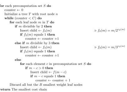
We use a newer algorithm to generate double-base chains, shown in Figure 7.1. This algorithm is an improved version of the basic “tree-based” algorithm pro-posed and analyzed by Doche and Habsieger in [21].
In the basic algorithm,nis computed recursively from either (n−1)/(2···3···) or
(n+ 1)/(2···3···), where the exponents of 2 and 3 are chosen to be as large as pos-sible. The algorithm explores the branching tree of possibilities in breadth-first fashion until it reaches n = 1. To limit time and memory usage, the algorithm keeps only the smallest B nodes at each level. We chose B = 200.
We use an extension to this algorithm mentioned but not analyzed in [21]. The extension uses not just n−1 and n+ 1, but all n−c where c is in a pre-computed set (including both positive and negative values). We include the cost of precomputing this set. We chose 21 different possibilities for the precomputed set, namely the 21 sets listed in [6].
We change the way to add new nodes as follows:
– n has one child noden/2 if n is divisible by 2;
– otherwise, n has one child node n/3 if n is divisible by 3;
Input: An integern, precomputation set S, and boundsB andC Output: A double-base chain computingn
for each precomputation setS do counter ←0
Initialize a tree T with root noden while (counter < C) do
for each leaf nodemin T do if mdivisible by 2 then
Insert child ←f2(m) . f2(m) =m/2v2(m)
if f2(m) equals 1then
counter←counter +1 else if mdivisible by 3 then
Insert child ←f3(m) . f3(m) =m/3v3(m)
if f3(m) equals 1then
counter←counter +1 else
for each elementc in precomputation setS do if m−c >0then
Insert child←f(m−c) if m−c equals 1then
counter←counter + 1
Discard all but the B smallest weight leaf nodes return The smallest cost chain
Fig. 7.1.The algorithm we used to generate double-base chains. “End” statements are implied by indentation, as in Python.
We improve the algorithm by continuing to search the tree until we have found C chains, rather than stopping with the first chain; we then take the lowest-cost chain. We chose C = 200.
We further improve the algorithm by taking the lowest-weight B nodes at each level instead of the smallest B nodes at each level; here “weight” takes account not just of smallness but also of the cost of operations used to reach the node. More precisely, we define “weight” as cost + 8·log2(n).
We ran this algorithm for 10000 random 256-bit scalars, i.e., integers between 2255 and 2256 −1, using as input the costs of twisted Hessian operations. The average cost of the resulting chain was 8.77M per bit.
-50 0 50 100
0 50 100 150 200 250 300 350 400 450 500 550 600 650
Multiplications saved
Multiplications using the new formulas
-100 -50 0 50
0 50 100 150 200 250 300 350 400 450 500 550 600 650
Multiplications saved
Multiplications using the new formulas
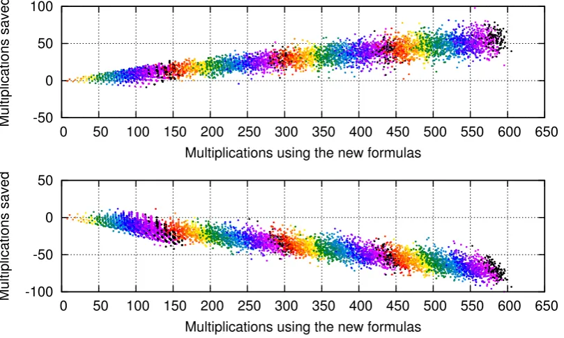
Fig. 7.2. Top: Points (x, y) for 100 randomly sampled b-bit integers n for each b ∈ {2,3, . . . ,64}. Here xM are used to compute P 7→nP on a twisted Hessian curve in projective coordinates; (x+y)Mare used to computeP 7→nP on a Weierstrass curve y2 = x3−3x+a6 in Jacobian coordinates; and the color is a function of b. Bottom:
Similar, but using a twisted Edwards curve rather than a Weierstrass curve.
Weierstrass curve; i.e., switching from Weierstrass to twisted Hessian savesyM. We reduced the number of dots plotted in this figure to avoid excessive PDF file sizes and display times, but a full plot is similar. Dots along thex-axis represent integers with the same cost for both curve shapes. Different colors are used for different bit-sizes b.
We have generated similar plots for some other pairs of curve shapes. For example, the bottom of Figure 7.2 shows that Edwards is faster than Hessian for most values of n. In some cases, such as Hessian vs. tripling-oriented Doche– Icart–Kohel curves, the plots are concentrated much more narrowly around a line, since these curve shapes favor similar integers that use many triplings; the line has a positive slope, i.e., Hessian is faster.
References
[1] Christophe Ar`ene, Tanja Lange, Michael Naehrig, Christophe Ritzenthaler,Faster computation of the Tate pairing, Journal of Number Theory131(2011), 842–857. URL:https://eprint.iacr.org/2009/155. Citations in this document:§2. [2] Siegfried Heinrich Aronhold, Zur Theorie der homogenen Functionen
view/j/crll.1850.issue-39/crll.1850.39.140/crll.1850.39.140.xml. Cita-tions in this document: §2.
[3] Josh Benaloh (editor), Topics in cryptology — CT-RSA 2014 — the cryptogra-pher’s track at the RSA Conference 2014, San Francisco, CA, USA, February 25–28, 2014, proceedings, Lecture Notes in Computer Science, vol. 8366, Springer, 2014. ISBN 978-3-319-04851-2. See [27].
[4] Daniel J. Bernstein,Complete addition laws for all elliptic curves over finite fields (talk slides)(2009). URL:http://cr.yp.to/talks/2009.07.17/slides.pdf. Ci-tations in this document:§1.
[5] Daniel J. Bernstein,Curve25519: new Diffie-Hellman speed records, in PKC 2006 [52] (2006), 207–228. URL: http://cr.yp.to/papers.html#curve25519. Cita-tions in this document: §1.
[6] Daniel J. Bernstein, Peter Birkner, Tanja Lange, Christiane Peters, Optimiz-ing double-base elliptic-curve sOptimiz-ingle-scalar multiplication, in Indocrypt 2007 [51] (2007), 167–182. URL: https://eprint.iacr.org/2007/414. Citations in this document:§1,§7,§7.
[7] Daniel J. Bernstein, Niels Duif, Tanja Lange, Peter Schwabe, Bo-Yin Yang, High-speed high-security signatures, Journal of Cryptographic Engineering 2 (2012), 77–89. URL: https://eprint.iacr.org/2011/368. Citations in this document: §1.
[8] Daniel J. Bernstein, Tanja Lange, Explicit-formulas database (2007). URL:
https://hyperelliptic.org/EFD. Citations in this document: §1.
[9] Daniel J. Bernstein, Tanja Lange, Faster addition and doubling on elliptic curves, in Asiacrypt 2007 [40] (2007), 29–50. URL: http://cr.yp.to/papers. html#newelliptic. Citations in this document: §1, §1.
[10] Daniel J. Bernstein, Tanja Lange, Analysis and optimization of elliptic-curve single-scalar multiplication, in Fq8 [44] (2008), 1–19. URL: https://eprint. iacr.org/2007/455. Citations in this document: §1.
[11] Daniel J. Bernstein, Tanja Lange,A complete set of addition laws for incomplete Edwards curves, Journal of Number Theory131(2011), 858–872. URL: http:// cr.yp.to/papers.html#completed. Citations in this document: §4,§4,§4,§4. [12] Guido Bertoni, Jean-S´ebastien Coron (editors), Cryptographic hardware and
em-bedded systems — CHES 2013 — 15th international workshop, Santa Barbara, CA, USA, August 20–23, 2013, proceedings, Lecture Notes in Computer Science, vol. 8086, Springer, 2013. ISBN 978-3-642-40348-4. See [49].
[13] Olivier Billet, Marc Joye,The Jacobi model of an elliptic curve and side-channel analysis, in AAECC 2003 [28] (2003), 34–42. MR 2005c:94045. URL: eprint. iacr.org/2002/125. Citations in this document: §1.
[14] Wieb Bosma, Hendrik W. Lenstra, Jr.,Complete systems of two addition laws for elliptic curves, Journal of Number Theory 53(1995), 229–240. ISSN 0022–314X. MR 96f:11079. Citations in this document: §3,§3,§4,§4.
[15] Ljiljana Brankovic, Willy Susilo (editors),Australasian information security con-ference (AISC 2009), Wellington, New Zealand, January 2009, Conferences in Research and Practice in Information Technology (CRPIT), vol. 98, Australian Computer Society, Inc., 2009. See [31].
[16] Arthur Cayley, On the 34 concomitants of the ternary cubic, American Journal of Mathematics4(1881), 1–15. Citations in this document: §2.
[18] Henri Cohen, Gerhard Frey (editors),Handbook of elliptic and hyperelliptic curve cryptography, CRC Press, 2005. ISBN 1-58488-518-1. MR 2007f:14020. See [23]. [19] Henri Cohen, Atsuko Miyaji, Takatoshi Ono, Efficient elliptic curve
exponentia-tion using mixed coordinates, in Asiacrypt 1998 [48] (1998), 51–65. MR 1726152. URL: http://www.math.u-bordeaux.fr/~cohen/asiacrypt98.dvi. Citations in this document: §1.
[20] Craig Costello, Huseyin Hisil, Benjamin Smith, Faster compact Diffie–Hellman: endomorphisms on the x-line, in Eurocrypt 2014 [45] (2014), 183–200. URL:
https://eprint.iacr.org/2013/692. Citations in this document: §1.
[21] Christophe Doche, Laurent Habsieger, A tree-based approach for computing double-base chains, in ACISP 2008 [43] (2008), 433–446. Citations in this docu-ment: §1, §1,§7,§7.
[22] Christophe Doche, Thomas Icart, David R. Kohel,Efficient scalar multiplication by isogeny decompositions, in PKC 2006 [52] (2006), 191–206. Citations in this document:§1.
[23] Christophe Doche, Tanja Lange, Arithmetic of elliptic curves, in HEHCC [18] (2005), 267–302. Citations in this document:§5.
[24] Harold M. Edwards, A normal form for elliptic curves, Bulletin of the Ameri-can Mathematical Society44(2007), 393–422. URL:http://www.ams.org/bull/ 2007-44-03/S0273-0979-07-01153-6/home.html. Citations in this document:§1. [25] Reza Rezaeian Farashahi, Marc Joye,Efficient arithmetic on Hessian curves, in
PKC 2010 [46] (2010), 243–260. Citations in this document:§1,§1.
[26] Reza Rezaeian Farashahi, Hongfeng Wu, Chang-An Zhao,Efficient arithmetic on elliptic curves over fields of characteristic three, in SAC 2012 [35] (2013), 135–148. Citations in this document: §1,§1.
[27] Armando Faz-Hern´andez, Patrick Longa, Ana H. S´anchez, Efficient and secure algorithms for based scalar multiplication and their implementation on GLV-GLS curves, in CT-RSA 2014 [3] (2013), 1–27. URL:https://eprint.iacr.org/ 2013/158. Citations in this document: §1.
[28] Marc Fossorier, Tom Hoeholdt, Alain Poli (editors), Applied algebra, alge-braic algorithms and error-correcting codes, Lecture Notes in Computer Science, vol. 2643, Springer, 2003. ISBN 3-540-40111-3. MR 2004j:94001. See [13].
[29] Otto Hesse,Uber die Elimination der Variabeln aus drei algebraischen Gleichun-¨ gen vom zweiten Grade mit zwei Variabeln, Journal f¨ur die Reine und Angewandte Mathematik 28 (1844), 68–96. ISSN 0075-4102. Citations in this document: §2. [30] Huseyin Hisil, Gary Carter, Ed Dawson,New formulae for efficient elliptic curve
arithmetic, in Indocrypt 2007 [51] (2007), 138–151. Citations in this document: §1,§1,§1,§1,§6.
[31] Huseyin Hisil, Kenneth Koon-Ho Wong, Gary Carter, Ed Dawson, Faster group operations on elliptic curves, in AISC 2009 [15] (2009), 7-19. URL: https:// eprint.iacr.org/2007/441. Citations in this document: §1.
[32] Huseyin Hisil,Elliptic curves, group law, and efficient computation, Ph.D. thesis, Queensland University of Technology, 2010. Citations in this document: §1, §1, §1,§1.
[33] Dale Husem¨oller, Elliptic curves, 2nd edition, Graduate Texts in Mathematics, vol. 111, Springer, 2003. ISBN 978-0387954905. Citations in this document: §2. [34] Marc Joye, Jean-Jacques Quisquater, Hessian elliptic curves and side-channel
[35] Lars R. Knudsen, Huapeng Wu (editors), Selected areas in cryptography, 19th international conference, SAC 2012, Windsor, ON, Canada, August 15–16, 2012, revised selected papers, Lecture Notes in Computer Science, vol. 7707, Springer, 2013. ISBN 978-3-642-35998-9. See [26].
[36] Neal Koblitz,Algebraic aspects of cryptography, Algorithms and Computation in Mathematics, vol. 3, Springer, 1998. ISBN 978-3-540-63446-1. Citations in this document:§2.
[37] C¸ etin Kaya Ko¸c, David Naccache, Christof Paar (editors),Cryptographic hardware and embedded systems—CHES 2001, third international workshop, Paris, France, May 14–16, 2001, proceedings, Lecture Notes in Computer Science, vol. 2162, Springer, 2001. ISBN 3-540-42521-7. MR 2003g:94002. See [34], [41], [50].
[38] David Kohel,Addition law structure of elliptic curves, Journal of Number Theory 131(2011), 894–919. Citations in this document: §3.
[39] David Kohel, The geometry of efficient arithmetic on elliptic curves, in Arith-metic, Geometry, Coding Theory and Cryptography 637 (2015). Citations in this document: §1, §1,§1,§6.
[40] Kaoru Kurosawa (editor),Advances in cryptology—ASIACRYPT 2007, 13th in-ternational conference on the theory and application of cryptology and information security, Kuching, Malaysia, December 2–6, 2007, proceedings, Lecture Notes in Computer Science, vol. 4833, Springer, 2007. ISBN 978-3-540-76899-9. See [9]. [41] Pierre-Yvan Liardet, Nigel P. Smart,Preventing SPA/DPA in ECC systems using
the Jacobi form, in CHES 2001 [37] (2001), 391–401. MR 2003k:94033. Citations in this document: §1.
[42] Peter L. Montgomery,Speeding the Pollard and elliptic curve methods of factor-ization, Mathematics of Computation 48 (1987), 243–264. ISSN 0025-5718. MR 88e:11130. Citations in this document: §1.
[43] Yi Mu, Willy Susilo, Jennifer Seberry (editors), Information security and privacy — 13th Australasian conference, ACISP 2008, Wollongong, Australia, July 7–9, 2008, proceedings, Lecture Notes in Computer Science, vol. 5107, Springer, 2008. ISBN 978-3-540-69971-2. See [21].
[44] Gary L. Mullen, Daniel Panario, Igor E. Shparlinski (editors), Finite fields and applications: papers from the 8th international conference held in Melbourne, July 9–13, 2007, Contemporary Mathematics, vol. 461, American Mathematical Soci-ety, 2008. ISBN 978-0-8218-4309-3. MR 2009h:11004. See [10].
[45] Phong Q. Nguyen, Elisabeth Oswald (editors), Advances in cryptology — EUROCRYPT 2014 — 33rd annual international conference on the theory and ap-plications of cryptographic techniques, Copenhagen, Denmark, May 11–15, 2014, proceedings, Lecture Notes in Computer Science, vol. 8441, Springer, 2014. ISBN 978-3-642-55219-9. See [20].
[46] Phong Q. Nguyen, David Pointcheval (editors), Public key cryptography—PKC 2010, 13th international conference on practice and theory in public key cryptog-raphy, Paris, France, May 26–28, 2010, proceedings, Lecture Notes in Computer Science, vol. 6056, Springer, 2010. ISBN 978-3-642-13012-0. See [25].
[47] National Institute of Standards and Technology, Recommended elliptic curves for federal government use (1999). URL: http://csrc.nist.gov/groups/ST/ toolkit/documents/dss/NISTReCur.pdf. Citations in this document: §1.
[49] Thomaz Oliveira, Julio L´opez, Diego F. Aranha, Francisco Rodr´ıguez-Henr´ıquez,
Lambda coordinates for binary elliptic curves, in CHES 2013 [12] (2013), 311–330. URL:https://eprint.iacr.org/2013/131. Citations in this document:§1. [50] Nigel P. Smart,The Hessian form of an elliptic curve, in CHES 2001 [37] (2001),
118–125. Citations in this document: §2,§5.
[51] Kannan Srinathan, C. Pandu Rangan, Moti Yung (editors), Progress in cryptology—INDOCRYPT 2007, 8th international conference on cryptology in India, Chennai, India, December 9–13, 2007, proceedings, Lecture Notes in Com-puter Science, vol. 4859, Springer, 2007. ISBN 978-3-540-77025-1. See [6], [30]. [52] Moti Yung, Yevgeniy Dodis, Aggelos Kiayias, Tal Malkin (editors), Public key