Scholarship@Western
Scholarship@Western
Electronic Thesis and Dissertation Repository
9-5-2013 12:00 AM
Second-order Analysis of Cable-stayed Bridge Deck Slabs
Second-order Analysis of Cable-stayed Bridge Deck Slabs
Zachary McNeil
The University of Western Ontario
Supervisor
Dr. F. Michael Bartlett
The University of Western Ontario
Graduate Program in Civil and Environmental Engineering
A thesis submitted in partial fulfillment of the requirements for the degree in Master of Engineering Science
© Zachary McNeil 2013
Follow this and additional works at: https://ir.lib.uwo.ca/etd
Part of the Structural Engineering Commons
Recommended Citation Recommended Citation
McNeil, Zachary, "Second-order Analysis of Cable-stayed Bridge Deck Slabs" (2013). Electronic Thesis and Dissertation Repository. 1621.
https://ir.lib.uwo.ca/etd/1621
This Dissertation/Thesis is brought to you for free and open access by Scholarship@Western. It has been accepted for inclusion in Electronic Thesis and Dissertation Repository by an authorized administrator of
(Thesis format: Monograph)
by
Zachary McNeil
Graduate Program in Civil and Environmental Engineering
A thesis submitted in partial fulfillment of the requirements for the degree of
Master of Engineering Science
The School of Graduate and Postdoctoral Studies The University of Western Ontario
London, Ontario, Canada September 2013
ii
Current provisions in CSA S6-06 “Canadian Highway Bridge Design Code” for computing second-order effects in slender concrete beam-columns were derived for columns in buildings, where these effects can often be neglected, so their applicability to extremely slender cable-stayed bridge decks warrants investigation. The research reported in this thesis first reviews the provisions in CSA S6-06, as well as eight equations proposed by others, for computing the flexural rigidity, EI, of slender concrete beam-columns. Methods for quantifying the rotational restraint provided at deck slab supports by steel or concrete floorbeams are presented and validated: steel floorbeams provide negligible restraint but concrete floorbeams can provide sufficient restraint to reduce markedly the effective length factor. A rational method is presented and validated for analyzing continuous beam-columns subjected to transverse loads applied between their supports. A sensitivity analysis demonstrates that the variables that influence the moment magnification of cable-stayed bridge decks are: the applied axial load, the slenderness ratio, the concrete compressive strength, and the rotational restraint provided at the deck slab supports. Lastly, the deficiency of the provisions in CSA S6-06 for designing a simplified three-span cable-stayed bridge deck is demonstrated and recommendations are given to facilitate design office practice.
iii
To my supervisor, Dr. Mike Bartlett, I am especially grateful. Dr. Bartlett’s continuous guidance and cheerful encouragement have been invaluable during the past two years. His passion for structural engineering is inspirational and his dedication to his students and to the university is remarkable.
I would also like to thank Don Bergman from Buckland & Taylor Ltd. for his guidance regarding the axial stresses that are typical in cable-stayed bridge decks.
Financial support received from the National Science and Engineering Research Council of Canada and the Queen Elizabeth II Graduate Scholarship Program is gratefully acknowledged.
iv
PAGE
Abstract ... ii
Acknowledgements ... iii
Table of Contents ...iv
List of Tables ...vi
List of Figures ... vii
Nomenclature ...xi
Chapter 1: Introduction ... 1
1.1 Introduction ... 1
1.2 Slender Concrete Beam-columns ... 6
1.3 Slender Columns in CSA S6-06 ... 12
1.4 Instability of Cable-stayed Bridge Decks ... 14
1.5 Research Objectives ... 15
1.6 Thesis Outline ... 15
Chapter 2: Review of Slender Column Analyses in the Literature ... 17
2.1 Simplified EI Equations Proposed in the Literature ... 17
2.2 Influence of Key Variables on the Simplified EI Equations ... 23
2.3 Case Study: Variability among the EI Equations Proposed in the Literature ... 30
2.4 Summary and Conclusions ... 36
Chapter 3: Effective Length of Cable-stayed Bridge Decks ... 39
3.1 Introduction ... 39
3.2 Idealization of the Rotational Restraint of Transverse Floorbeams... 40
3.3 Approximate Analytical Equations for the Rotational Restraint of Transverse Floorbeams ... 41
3.4 Validation Using SAP2000 ... 44
3.5 Case Studies: The Effective Length of Deck Slabs with Steel and Concrete Floorbeams ... 47
3.6 Summary and Conclusions ... 54
Chapter 4: Second-order Analysis of Cable-stayed Bridge Decks with Non-uniform Primary Moment Diagrams ... 56
4.1 Idealized Structure ... 56
4.2 Moment-curvature Relationship ... 57
4.3 Moment Distribution at Supports... 59
4.4 Deflected Shape and Second-order Bending Moments ... 65
4.5 Maximum First-order Primary Moment ... 68
4.6 Overview of Computer Program ... 69
4.7 Validation ... 73
v
5.2 Analytical Approaches ... 83
5.3 Scope of the Sensitivity Analysis ... 86
5.3.1 Parameters Investigated ... 86
5.3.2 Applied Loading ... 90
5.4 CSDECK Results for Various Applied Axial Load Ratios ... 93
5.5 CSDECK Results for Various Slenderness Ratios ... 102
5.6 CSDECK Results for Various Concrete Compressive Strengths ... 108
5.7 CSDECK Results for Various Floorbeam Rotational Restraints ... 110
5.8 CSDECK Results for Various Reinforcing Ratios and Steel Depths ... 114
5.9 Accuracy of Simplified Design Methods ... 116
5.10 Summary ... 118
5.11 Conclusions ... 119
Chapter 6: Summary and Conclusions ... 123
6.1 Summary ... 123
6.2 Conclusions ... 125
6.3 Recommendations for Design Office Practice ... 129
6.4 Recommendations for Future Work... 131
References ... 133
Basis of Rigidity Equations Proposed by Others ... 136
Appendix A: Derivation of Approximate Equations for Computing the Appendix B: Rotational Restraint Provided by Floorbeams ... 147
Source Code for CSDECK ... 153
Appendix C: Sensitivity Analysis Results For Single-point-load Case ... 174
vi
PAGE Table 2.1: Proposed equations for the rigidity, EI. ... 17 Table 2.2: Variables included in the proposed rigidity equations... 23 Table 2.3: Maximum end moments obtained using the rigidity equations proposed in
the literature for C=1000kN. ... 34 Table 2.4: Maximum end moments obtained using the rigidity equations proposed in
the literature for C=5000kN. ... 36
Table 3.1: Rotational restraint provided by floorbeams. ... 44 Table 3.2: Upper- and lower-bound cross-sectional properties of steel and concrete
floorbeams. ... 49 Table 3.3: Rotational restraint bounds for bridges with steel and concrete
floorbeams. ... 50
vii
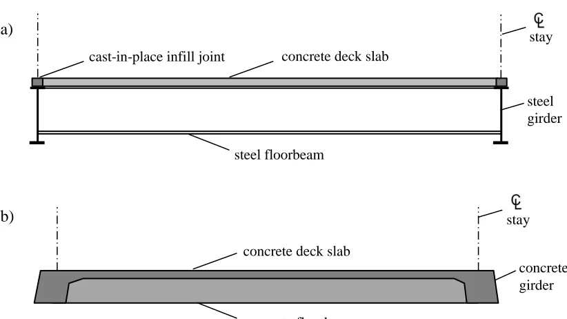
PAGE Figure 1.1: Cable-stayed bridge girder cross sections: a) composite girder system; b)
concrete girder system. ... 2 Figure 1.2: Simple cable-stayed bridge including typical a) global axial force
diagram, b) global bending moment envelope (from Gimsing &
Georgakis, 2012), c) global force effects on sections of the girder, and d) local force effects on the deck slab. ... 3 Figure 1.3: The maximum compressive stress in the girder system due to axial
compression and lateral bending (after Gimsing & Georgakis, 2012). ... 5 Figure 1.4: Forces on a simple slender column (after MacGregor & Bartlett, 2000). ... 7 Figure 1.5: Cross-section interaction diagram showing the responses of a short
column, A, an intermediate column, B, and a very slender column, C. ... 8 Figure 1.6: Relationship between the moment-curvature response and the secant and
tangent rigidities. ... 9 Figure 1.7: Moment-curvature response of a member susceptible to instability (after
Bartlett, 1991). ... 11
Figure 2.1: Interaction diagram showing Shuraim and Naaman’s (2003) proposal for calculating the secant rigidity using Eq. [1.3]. ... 20 Figure 2.2: The rigidity using the method proposed by Shuraim and Naaman
compared to results from their finite element analysis (from Shuraim & Naaman, 2003). ... 21 Figure 2.3: Effective rigidity according to Eq. [2.1] for short-term loading. ... 25 Figure 2.4: Influence of the normalized applied axial load, according to Eq. [1.3], on
the: a) rigidity; b) neutral axis depth; and c) moment resistance for ρg = 1% and f 'c 50MPa. ... 26 Figure 2.5: The variable rigidity factor, α, provided by Eq. [2.6] for short-term
loading. ... 29 Figure 2.6: Simply supported column: a) applied loading; b) cross section; c)
cross-section interaction diagram. ... 31 Figure 2.7: Cross-section interaction diagrams obtained using the provisions in CSA
S6-06 and the program CSDECK. ... 33
Figure 3.1: Deck slab instability: a) buckled shape; b) idealization with deck slab at floorbeam centroid. ... 39 Figure 3.2: Horizontal deflection of floorbeam centroid. ... 41 Figure 3.3: Concrete deck on steel floorbeams: a) plan; b) end elevation; and c) side
elevation. ... 43 Figure 3.4: Model specimen: a) cross section showing rigid link connecting the
viii
mm). ... 47 Figure 3.7: Effective length factors for cable-stayed bridge decks. ... 51
Figure 4.1: Cable-stayed bridge deck: a) cross section; b) idealized... 56 Figure 4.2: a) Curvature contours; b) moment-curvature relationship for C =
3000kN. ... 57 Figure 4.3: The force method of analysis, a) actual structure; b) primary structure; c)
redundant moment at the left interior support. ... 60 Figure 4.4: Flowchart for distributing moments in cable-stayed bridge decks. ... 64 Figure 4.5: Deflected shape of a small segment of a beam-column. ... 66 Figure 4.6: Flowchart for computing the total moment distribution of cable-stayed
bridge decks. ... 68 Figure 4.7: Maximum possible primary moment. ... 69 Figure 4.8: Hierarchy of the MATLAB program developed. ... 71 Figure 4.9: Cable-stayed bridge deck; a) cross section; b) idealized structural system
(dimensions in mm). ... 74 Figure 4.10: Bending moment diagrams from ANSYS 12.0; a) total; b)
second-order; and c) total and first-order. ... 77 Figure 4.11: Total moment diagrams obtained from ANSYS 12.0 and the MATLAB
program. ... 78
Figure 5.1: First- and second-order moment diagrams; a) L/r = 107; b) L/r = 49. ... 84 Figure 5.2: Cable-stayed bridge deck loading: a) uniformly distributed; b) two point
loads spaced at L/3; c) super-imposed moment diagrams. ... 92 Figure 5.3: Idealized cable-stayed bridge deck used to perform a sensitivity analysis. .. 92 Figure 5.4: Moment magnifier for various applied axial load ratios when f'c=
55MPa, using: a) noncracked first-order analysis; b)
linear-uncracked first-order analysis. ... 93 Figure 5.5: Moment-curvature relationships for two applied axial loads. ... 95 Figure 5.6: Ratio of moment magnifiers computed using a linear-uncracked
first-order analysis to those using a nonlinear-cracked first-first-order analysis. ... 97 Figure 5.7: a) Beam elevation; b) first-order rigidity distribution; c) linear-uncracked
first-order curvature diagram; d) nonlinear-cracked first-order curvature diagram. ... 98 Figure 5.8: Moment curvature relationship for C = 0.4 'f c Ag. ... 100 Figure 5.9: Moment curvature relationship for C = 0.6 'f c Ag. ... 101 Figure 5.10: Moment magnifier for various slenderness ratios when f'c = 55MPa,
using: a) noncracked first-order moment diagram; b)
ix
Figure 5.12: Ratio of moment magnifiers computed using a linear-uncracked first-order analysis and a nonlinear-cracked first-first-order analysis for various
slenderness ratios. ... 106 Figure 5.13: Moment magnifier for various concrete compressive strengths when L/r
= 80, using: a) noncracked first-order moment diagram; b) linear-uncracked first-order moment diagram. ... 108 Figure 5.14: Moment magnifiers from a nonlinear-cracked first-order analysis for
various floorbeam rotational restraints; a) L/r = 60; b) L/r = 80; c) L/r = 100. ... 111 Figure 5.15: Ratio of moment magnifiers computed using a linear-uncracked
first-order analysis and a nonlinear-cracked first-first-order analysis for various
rotational restraints; L/r = 60. ... 113 Figure 5.16: Moment magnifiers for various reinforcing ratios when L/r = 80, using:
a) nonlinear-cracked first-order moment diagram; b) linear-uncracked
first-order moment diagram. ... 115 Figure 5.17: Moment magnifiers for various steel-depth-to-slab-thickness ratios
when L/r = 80, using the following first-order analyses: a)
nonlinear-cracked; b) linear-uncracked. ... 116
Figure A.1: The real load path of a stability failure and the simulated load path
assumed by Nathan (after Nathan, 1983). ... 137 Figure A.2: The moment resistance vs. extreme fibre compressive strain relationship
for a 400mm square column, f'c = 30MPa and g= 2%. ... 140
Figure C.1: Iterations of distributing moments in the interior span. ... 164
Figure D.1: Moment magnifier for various applied axial load ratios when f’c = 55MPa, using the following first-order analyses: a) nonlinear-cracked; b) linear-uncracked. ... 175 Figure D.2: Ratio of moment magnifiers computed for various applied axial loads
using a linear-uncracked first-order analysis to those using a
nonlinear-cracked first-order analysis. ... 176 Figure D.3: Moment magnifier for various slenderness ratios when f'c = 55MPa,
using the following first-order analyses: a) noncracked; b) linear-uncracked. ... 177 Figure D.4: Ratio of moment magnifiers computed using a linear-uncracked
first-order analysis and a nonlinear-cracked first-first-order analysis for various
x
first-order analysis. ... 179 Figure D.6: Moment magnifiers from a nonlinear-cracked first-order analysis for
various floorbeam rotational restraints; a) L/r = 60; b) L/r = 80; c) L/r = 100. ... 180 Figure D.7: Ratio of moment magnifiers computed using a linear-uncracked
first-order analysis and a nonlinear-cracked first-first-order analysis for various
rotational restraints; L/r = 60. ... 181 Figure D.8: Moment magnifiers for various reinforcing ratios, using the following
first-order analyses: a) nonlinear-cracked b) linear-uncracked... 182 Figure D.9: Moment magnifiers for various steel-depth-to-slab-thickness ratios,
xi Ag area of the gross concrete section As area of tension steel reinforcement A’s area of compression steel reinforcement a distance from the support to the applied load be effective flange width
C applied compression force Cc critical buckling load Cf factored axial load
Co axial resistance of the cross section for zero applied moment Cu ultimate cross-sectional axial load resistance
cm non-uniform moment factor
cu neutral axis depth at the ultimate limit state d depth of reinforcement
Ec modulus of elasticity of concrete
Es modulus of elasticity of steel reinforcement Esc secant modulus of elasticity of concrete Etc tangent modulus of elasticity of concrete EcIg uncracked rigidity
EIsec secant rigidity EItan tangent rigidity EI flexural rigidity
e first-order end eccentricity c
f' 28-day concrete compressive strength fc concrete stress
fy yield stress of steel reinforcement
fLL flexibility coefficient for the left interior support due to a moment at the left interior support
fLR flexibility coefficient for the left interior support due to a moment at the right interior support
fRL flexibility coefficient for the right interior support due to a moment at the left interior support
fRR flexibility coefficient for the right interior support due to a moment at the right interior support
G shear modulus of elasticity
Gc shear modulus of elasticity of concrete
H height of cable-stayed bridge tower above the deck h height of the cross section
hs deck slab thickness J torsional constant
xii Iy moment of inertia about the y-axis
Ke rotational restraint provided by the vertical eccentricity of the deck slab Kθ rotational restraint provided by the transverse floorbeams
kθ rotational restraint per unit width of slab provided by the transverse floorbeams k effective length factor
kG flexural stiffness accounting for second-order effects (kGL: left adjacent span; kGR: right adjacent span)
L compression member length, equivalent to the floorbeam spacing Lm main span length
M bending moment
Mc maximum total moment at the critical section (Mc,A: actual value; Mc,S: simulated value)
Md decompression moment
Mu ultimate cross-sectional moment capacity My yield moment
ML moment at the left interior support MR moment at the right interior support M* total moment
M2 maximum applied first-order end moment
M2* maximum applied first-order end moment computed using CSDECK P applied vertical point load
Pe restraining force provided by the vertical eccentricity of the deck slab pe uniform restraint provided by the vertical eccentricity of the deck slab r radius of gyration
s spacing of the longitudinal girders T applied torque
Te restraining torque provided by the vertical eccentricity of the deck slab UBC upper-bound property for concrete floorbeams
UBS upper-bound property for steel floorbeams LBC lower-bound property for concrete floorbeams LBS lower-bound property for steel floorbeams w slab width
xiii
α variable rigidity factor in equations proposed by others β coefficient in rigidity equations by Tikka and Mirza (2008) βd sustained load factor
β1 ratio of equivalent stress block depth to the neutral axis depth
γL modification factor to account for second-order effects in the left adjacent span γR modification factor to account for second-order effects in the right adjacent span δ moment magnifier (δL: computed using linear-uncracked first-order analysis; δNL:
computed using nonlinear-cracked first-order analysis) Δ deflection
Δe deflection of floorbeam centroid due to the vertical eccentricity of the deck slab ε strain
εc extreme compression fibre strain (εcu: at the ultimate limit state) εo strain corresponding to the peak concrete stress
η coefficient in rigidity equation by Nathan (1983)
ηe relative eccentricity factor in rigidity equation by Bonet et al. (2011) θ rotation
θL primary rotation at the left end of the interior span θR primary rotation at the right end of the interior span
θLL rotation at the left end of the interior span due to the unit moment at the left interior support
θ’LL rotation at the right end of the left adjacent span due to the unit moment at the left interior support
θRR rotation at the right end of the interior span due to the unit moment at the right interior support
θ’RR rotation at the left end of the right adjacent span due to the unit moment at the right interior support
θRL rotation at the right end of the interior span due to the unit moment at the left interior support
ξφ sustained load factor in rigidity equation proposed by Bonet et al. (2011) ρg gross reinforcement ratio
φ creep coefficient from Eurocode 2 ϕm member resistance factor
ψ curvature
ψc curvature at the critical section Ψ relative stiffness ratio
CHAPTER 1: INTRODUCTION
1.1 INTRODUCTION
Cable-stayed bridges are elegant structures that are economical for spans less than 1200m. The configuration has only recently been chosen for spans over 1000m that historically were the domain of the suspension bridge (Hauge & Anderson, 2011). As the pushing of the span envelope continues, the use of slender girder systems is no longer just an aesthetic preference but a necessity due to self-weight considerations.
Figure 1.1: Cable-stayed bridge girder cross sections: a) composite girder system; b) concrete girder system.
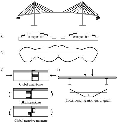
In both girder systems shown in Figure 1.1, the deck slab must resist local bending moments from traffic loads applied between floorbeams, compression forces due to global bending of the girder system, and additional compression forces from the horizontal component of the stay cable tensions, as shown in Figure 1.2. The global axial force diagram of a typical cable-stayed bridge, shown in Figure 1.2 a), generally has a parabolic shape with the maximum compression at the towers. The typical global bending moment diagram, shown in Figure 1.2 b), is characterized by positive moments larger than the negative moments in regions with significant compression and positive and negative moments of similar magnitude near midspan where the compression is the least (Gimsing & Georgakis, 2012). The deck slab will act as a compression flange for the girder system, resisting global axial loads and positive moments, as shown in Figure 1.2 c), but will only resist negative bending moments if there is sufficient axial force to prevent tensile stresses in the deck. The stress blocks in Figure 1.2 c) are shown at the
steel girder
a)
concrete deck slab cast-in-place infill joint
stay
b)
concrete deck slab
concrete floorbeam
ultimate limit state. The deck slabs spanning between the floorbeams also resist local moments resulting from traffic loads, shown in Figure 1.2 d), which will generally be positive beneath the applied load and negative above the supports.
Figure 1.2: Simple cable-stayed bridge including typical a) global axial force diagram, b) global bending moment envelope (from Gimsing & Georgakis, 2012), c) global force
effects on sections of the girder, and d) local force effects on the deck slab.
The maximum compression force at the towers due to the horizontal component of the stay cable tensions increases significantly as the main span length increases. For a fan
compression compression
a)
b)
c)
Global axial force
Global positive moment
Global negative moment
- +
+
- -
configuration, with all cables connected at the top of the tower, and uniform dead and live loads placed along the length of the main span, the maximum compression force, C, in the deck system is (Gimsing & Georgakis, 2012):
[1.1]
2
8
D L Lm
C
H
where ωD and ωL are uniformly distributed dead and live loads per unit length of deck, Lm is the main span length, and H is the height of the tower above the centroid of the deck system. For a constant uniformly distributed load, ωD+ωL, the compression force, C, should increase proportional to Lm, since the tower height, H, usually also increases proportionally to Lm (Gimsing & Georgakis, 2012). However, the increase in C requires a larger deck cross section, increasing the dead load per unit length, leading to a further increase in deck compression.
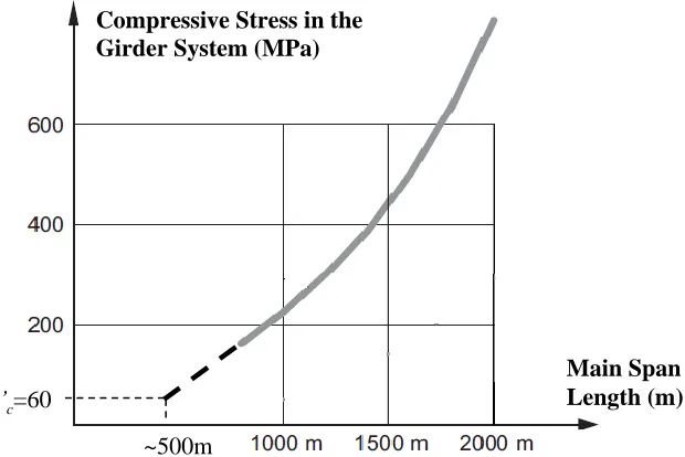
Figure 1.3 shows the approximate relationship between the compressive stress in the girder and main span length, proposed by Gimsing and Georgakis (2012) for a cable-stayed bridge with a constant deck width. The compressive stress is computed accounting for both the axial force from the horizontal component of the stay cable tensions and the additional stresses due to lateral bending of the girder system. The black-dashed line is a linear extrapolation of the original relationship and suggests that the span current limit for girder systems with concrete decks ( f'c≤60MPa) is in the order of 500m. For
girder system must be reduced. For composite girder systems, lightweight concrete is not a viable option since undesirable creep properties and reduced elastic moduli result from using lightweight aggregates (e.g., Lopez, 2005). Therefore, minimizing the deck slab thickness seems to be the most viable option, although innovative panel cross sections, such as fluted panels, could also be considered (Bergman, 2011).
Figure 1.3: The maximum compressive stress in the girder system due to axial compression and lateral bending (after Gimsing & Georgakis, 2012).
Given that the panels are subjected to combined bending and axial compression loads, they must be designed as slender beam-columns since slenderness ratios larger than 70 can occur in practice. The longest cable-stayed bridge in Canada, the Alex Fraser Bridge in Vancouver, has a main span of 465m and its 215mm thick precast panels have slenderness ratios of 73 (CBA-Buckland & Taylor Ltd, 1983). Currently the longest cable-stayed bridge in North America, the John James Audubon Bridge near New Roads, Louisiana, has a main span 482m and consists of 240mm precast panels with slenderness
Compressive Stress in the Girder System (MPa)
Main Span Length (m)
f’c=60
ratios of 66 (Schemmann et al., 2011). These members are extremely slender compared to typical building columns, where slenderness effects can usually be ignored (MacGregor, Breen, & Pfrang, 1970) and hence may require a more sophisticated analysis than is currently provided by Canadian standards.
1.2 SLENDER CONCRETE BEAM-COLUMNS
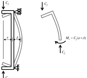
Figure 1.4: Forces on a simple slender column (after MacGregor & Bartlett, 2000).
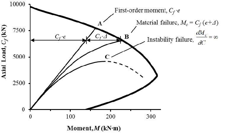
Significant second-order effects can results in two failure modes, as demonstrated by the axial load versus bending moment diagram shown in Figure 1.5. The bold outer line is the capacity of the cross section. A short column, with no moment magnification, follows the linear load path shown until reaching the cross-section capacity at point A. An intermediate column will follow a nonlinear path, due to the Cf -Δ effect, until it fails when the sectional strength is reached at point B. In both of these cases the cross-section capacity is reached, so the resistance of the column is limited by material failure. Slender (or “long”) columns will not reach material failure but will fail at a maximum moment less than the cross-section capacity where the increase in moment for an increase in axial load, dMc/dC, approaches infinity, as shown by point C. The moment magnification, due to the Cf - Δ effect, is usually very significant for long columns,
e Δ
Cf
Cf
Cf
Cf
causing an instability failure to occur before the cross-section capacity is achieved (MacGregor & Bartlett, 2000).
Figure 1.5: Cross-section interaction diagram showing the responses of a short column, A, an intermediate column, B, and a very slender column, C.
To further examine these failure modes, a distinction between secant and tangent member rigidities is necessary. Material failures are dependent on the moment magnification present and so on the secant rigidity at failure, EIsec, which is simply the moment, M, divided by the corresponding curvature, ψ:
[1.2] EIsec M
[1.3] u u sec
cu
M c
EI
ε
where the neutral axis depth at the ultimate limit states, cu, is determined for the ultimate cross-sectional moment capacity, Mu, and the strain in the extreme compression fibre, εcu, is assumed to be equal to 0.0035 in CSA S6-06.
As the applied moment increases, the secant rigidity reduces as shown by the moment-curvature curve in Figure 1.6. At instability failure, which depends on the tangent rigidity at the failure point A, the maximum moment is less than the cross-section capacity, Mu, and hence the secant stiffness is greater than at material failure.
Instability failure is dependent on the tangent rigidity of the member, dM/dψ, which is also shown on Figure 1.6. Bartlett (1991) and others have developed a rational expression for the mid-height tangent rigidity, dMc/dψc, at instability, using the Euler buckling formula:
[1.4]
2
2
f c tan
c
C kL
dM EI
dψ π
[1.5]
22 2
f
c c
C kL
M M ψ
π
Figure 1.7: Moment-curvature response of a member susceptible to instability (after Bartlett, 1991).
investigation is required to determine the response of continuous beam-columns subjected to non-uniform first-order moments.
1.3 SLENDER COLUMNS IN CSAS6-06
For reinforced concrete members with slenderness ratios less than 100, CSA S6-06 (CSA, 2006) allows slenderness effects to be computed using a moment magnifier, δ, computed as:
[1.6]
1
0.75
m f
c
c δ
C
C
The magnified moment, Mc, equivalent to Cf(e+Δ) in Figure 1.4, is computed as the product of the moment magnifier, δ, and the larger first-order end moment, M2. The factor, cm, accounts for unequal end moments and is taken as 1.0 for members with transverse loads applied between supports, such as traffic loads applied to the deck slabs of cable-stayed bridges. The 0.75 factor accounts for uncertainties in determining the critical buckling load (Bartlett, 1991), Cc, where Cc is the Euler Buckling Load given by:
[1.7]
22
c
π EI C
where EI is the rigidity and kL is the effective buckling length. For moment magnification, the rigidity of the column, EI, must represent the secant rigidity, which is approximated using two equations in CSA S6-06:
[1.8]
d
s s g c
β I E I E EI
1 2 . 0
[1.9] EI 0.25EcIg
In these equations, Ec and Es are the elastic moduli for concrete and steel respectively, and Ig and Is are the moments of inertia about the centroid of the section for the gross concrete section and the steel reinforcement, respectively. The factor βd accounts for the fraction of applied load that is sustained. Equation [1.8] is more accurate than Eq. [1.9], although for lightly reinforced concrete members the more conservative Eq. [1.9] tends to produce acceptable results (MacGregor, Breen, & Pfrang, 1970). The simplicity of Eq. [1.9] is often preferred during preliminary stages of design.
Provided it can be justified, CSA S6-06 allows the use of an effective length factor, k, less than 1 for members in braced frames. There is no guidance, however, for computing k for cable-stayed bridge deck slabs restrained by transverse floorbeams.
rigidity of the section at material failure. If a member fails by instability, the maximum moment will be less than the cross-section capacity, Mu, and the secant rigidity at failure will likely be much greater than that predicted by Eqs. [1.8] or [1.9], as was shown in Figure 1.6 (Bartlett, 1991).
1.4 INSTABILITY OF CABLE-STAYED BRIDGE DECKS
Very slender columns fail due to instability before the maximum moment along the member reaches the cross-section capacity, i.e. when dMc/dC=∞, as shown in Figure 1.5. Since the CSA S6-06 rigidity equations, Eqs. [1.8] and [1.9], were derived primarily for material failures, their extension to the analysis of instability failures is hard to justify. The inaccuracy associated with their use to compute the resistance of a cable-stayed bridge deck with a slenderness ratio of 73 was reported by Bartlett (1991). Slender column resistances computed using rigidity equations similar to those in CSA S6-06 were compared to those obtained by computing the critical mid-height moment associated with the critical tangent rigidity, Eq. [1.4], and the corresponding first-order end moment using Eq. [1.5]. The results varied significantly between the two approaches, with the code provisions providing extremely conservative resistances in the compression failure region and unconservative capacities in the tension failure region.
to more complex non-uniform loading conditions can also be expected to contain significant error, so other methods proposed in the literature must be examined.
1.5 RESEARCH OBJECTIVES
The objectives of this research are as follows:
1) Determine the accuracy of the current methods in the literature for computing the rigidity, EI, of slender concrete beam-columns.
2) Develop approximate methods for computing the rotational restraint provided by steel or concrete transverse floorbeams and apply these methods to compute the effective length of cable-stayed bridge decks.
3) Develop a rational method for computing first- and second-order moments in continuous, slender beam-columns subjected to transverse point loads between the supports.
4) Implement the method into a computer program capable of analyzing an idealized cable-stayed bridge deck system.
5) Perform a sensitivity analysis of the parameters that influence the moment magnification of continuous cable-stayed bridge decks.
6) Provide recommendations to practicing designers.
1.6 THESIS OUTLINE
CHAPTER 2: REVIEW OF SLENDER COLUMN ANALYSES IN THE LITERATURE
2.1 SIMPLIFIED EIEQUATIONS PROPOSED IN THE LITERATURE
Several equations for the effective rigidity, EI, of slender columns have been developed since the moment magnifier equation, Eq. [1.6], was introduced by MacGregor et al. in 1970. The equations in Table 2.1 include:
two rigidity equations provided in CSA S6-06, Eqs. [1.8] and [1.9],
six equations that have been proposed in the literature to replace the current
code equations, Eqs. [2.1] to [2.6],
one theoretical equation for the secant rigidity at material failure first
proposed by Anderson and Moustafa (1970), Eq. [1.3].
All equations yield nominal rigidities and, with the exception of Eq. [2.1], should be used with the stability resistance factor of 0.75, which accounts for uncertainties in determining the buckling load, Cc, in Eq. [1.6].
Table 2.1: Proposed equations for the rigidity, EI. Eq. [#] Author
(year)
General Form of
Equation Variable Rigidity Factors
[1.8] CSA (2006)
#1
0.2 1
c g s s d
E I E I EI
β
[1.9] CSA (2006)
Table 2.1 (cont.): Proposed equations for the rigidity, EI. Eq. [#] Author
(year)
General Form of
Equation Variable Rigidity Factors
[2.1] Nathan
(1983)
1
c g d E I EI α β 1.5 α ηΩ
23 0.02
7 100
f o f o
η
C C C C
η
Sections with no compression flange: 17 Ω kL r [2.2] Khuntia & Ghosh (2004)a
0.80 25
c g g
EIαE I ρ 1 0.5 f
o C e α h C
[2.3] Olendzki
(2008)
d
s s g c β I E I E α EI 1 4733 ' c c
E f
kLr
α0.810.004
[2.4]
Tikka & Mirza (2008) #1
0.85 1c g s
s s d
αE I I
EI E I
β
1
0.48 3.5 0.00058 1
e kL
α
e
h β r
h
7 for g 2%
β ρ
[2.5]
Tikka & Mirza (2008)
#2
0.8 1 c g s s d αE I
EI E I
β
1
0.47 3.5 0.00087 1
e kL
α
e
h β r
h
7 for g 2%
β ρ [2.6] Bonet, Romero & Miguel (2011)
1
(1 ) c g s sφ
αE I E I EI
φ ξ
' 10
0.3 000 , 22 c c f E 1.9 exp 25 φ kL ξ φ r 4 e e η r For ηe < 0.2:
1.95 0.035 0.25 0.2
'c 225 0.11 0.1
e kL φ η r f α
For ηe ≥ 0.2:
' 110 0.45 0.2
' 225 0.11 0.1
c c
e
α f η
f [1.3] Anderson & Moustafa (1970)a u u cu M c EI ε a
In Table 2.1, Ec and Es are the concrete and steel moduli of elasticity, respectively. The moments of inertia of the gross uncracked concrete section and the steel reinforcement are Ig and Is, respectively. The sustained load factor is βd, kL is the effective buckling length, and r is the radius of gyration. The eccentricity of the applied load, Cf,is e and Co is the factored axial resistance of the cross section for zero applied moment. The height of the cross section is h, ρg is the gross reinforcing ratio, and f'c is the 28-day concrete compressive strength in MPa. The creep coefficient used in Eq. [2.6], φ, is recommended by Bonet et al. (2011) to be taken from Eurocode 2 (European Committee for Standardization, 2004). The ultimate neutral axis depth, cu, in Eq. [1.3] corresponds to the cross-sectional moment resistance, Mu, at the applied load, Cf, and the ultimate strain in the extreme compression fibre, εcu, is assumed to be 0.0035 in CSA S6-06. Most of the equations contain a variable rigidity factor, α, as defined in the rightmost column.
A variation on Eq. [1.3] was suggested by Shuraim and Naaman (2003) for slender prestressed concrete columns. As shown in Figure 2.1, they propose adopting the secant rigidity corresponding to the applied end eccentricity, eM2 Cf , shown as point B,
instead of taking the rigidity at the applied load Cf, point A, as suggested by Anderson and Moustafa (1970).
Figure 2.1: Interaction diagram showing Shuraim and Naaman’s (2003) proposal for calculating the secant rigidity using Eq. [1.3].
[2.7]
1
2
3 u
h c
β
where β1 is the ratio of the equivalent rectangular stress block depth to the neutral axis depth.
Figure 2.2: The rigidity using the method proposed by Shuraim and Naaman compared to results from their finite element analysis (from Shuraim & Naaman, 2003).
the Cu and Mu corresponding to cu from Eq. [2.7]. Once both the Mu and cu values are known, the peak rigidity can be computed using Eq. [1.3].
For applied end eccentricities less than that corresponding to the peak rigidity, they propose computing the rigidity by interpolating between the peak secant rigidity, point B on Figure 2.2, and the tangent rigidity under concentric axial load, EItan, shown by the dashed line, which is computed as:
[2.8] EItanE Itc g
where Etc, the concrete tangent modulus of elasticity, computed as:
[2.9] 2 'c 1
tc
o ο
f ε
E
ε ε
where εo is the strain corresponding to the peak stress, f'c, and the strain, ε, at failure under concentric axial load is computed as:
[2.10]
2 4
2
o o
π r π r
ε ε ε
kL kL
2.2 INFLUENCE OF KEY VARIABLES ON THE SIMPLIFIED EIEQUATIONS
The equations shown in Table 2.1, except Eqs. [1.8] and [1.9], yield flexural rigidities that are not constant for a given cross section. There is little agreement regarding which
variables influence the rigidity, however, as shown in Table 2.2. The symbol
indicatesthat the equation neglects the contribution of a particular variable to the effective rigidity, while the symbol indicates the equation specifically addresses the instability case. A
plus,
, or minus sign,
, indicates that an increase in a particular variable will increaseor decrease the effective rigidity, respectively. As will be detailed in this section, there is limited consensus of which variables are important or how a particular variable impacts the rigidity.
Table 2.2: Variables included in the proposed rigidity equations. Eq. [#] Author (year) e f
o
C C
kL
r ρg or Is f'c or Ec
Address Instability
[1.8] CSA (2006) #1
[1.9] CSA (2006) #2
[2.1] Nathan (1983)
[2.2] Khuntia &
Ghosh (2004)
[2.3] Olendzki (2008)
[2.4] Tikka & Mirza
(2008) #1
[2.5] Tikka & Mirza
(2008) #2
[2.6] Bonet, Romero
& Miguel (2011)
/
[1.3] Anderson &
Moustafa (1970)
/
/
[1.3] & [2.8]
Shuraim &
All of the proposed methods account for the increase in effective rigidity resulting from an increase in the concrete modulus of elasticity, Ec, as shown in Table 2.2. All of the methods except the simplified CSA S6-06 Eq. [1.8] and Eq. [2.1] proposed by Nathan (1983) account for an increase in rigidity due to increased reinforcement, either ρg or Is.
In Eqs. [2.1], [2.4] and [2.5], and [2.6], the rigidity increases as the slenderness ratio, kL/r, increases. Increasing the slenderness increases the likelihood of an instability failure (e.g. Bonet et al., 2011) and the associated rigidity is greater. Clearly the rigidity used must correspond to the correct mid-height moment, Mc. Hence, the rigidity, EI, increases as the slenderness increases, because the mid-height moment at failure decreases. Equation [2.3] implies, however, that the rigidity will decrease as the slenderness increases, perhaps because it was developed entirely on statistical analyses.
Equation [2.1] implies that increasing Cf /Co will increase the rigidity, as shown in Figure 2.3 for various slenderness ratios, kL/r. At axial loads less than 0.02Co the rigidity from Eq. [2.1] is a minimum value, which is defined by the slenderness ratio. Equation [2.1] reaches a maximum at 0.42Co that is also related to the slenderness ratio. For columns with slenderness ratios exceeding 80, this maximum rigidity value is limited to two thirds of the gross rigidity, EcIg. Equation [2.2], contradicts Eq. [2.1] however, because it implies that the effective rigidity will reduce as the normalized applied axial load is increased.
Figure 2.3: Effective rigidity according to Eq. [2.1] for short-term loading.
c
f' = 50MPa, ρg= 1%, and d/h from 0.75 to 0.90. Since the top steel layer in cable-stayed bridge decks is not tied to prevent buckling, only the lower layer has been considered when computing the reinforcing ratio, ρg. Increasing the d/h ratio causes a slight increase in effective rigidity, as shown in Figure 2.4 a). Increasing the normalized applied axial load causes a more significant response, increasing the effective rigidity at low axial loads and decreasing it at higher loads. To further examine the influence of either the axial load or the d/h ratio on the secant rigidity, the effects of increasing these parameters on the neutral axis depth and on the cross-sectional moment resistance will be considered separately.
Figure 2.4: Influence of thenormalized applied axial load, according to Eq. [1.3], on the: a) rigidity; b) neutral axis depth; and c) moment resistance for ρg = 1% and f 'c 50MPa.
b) a)
Figure 2.4 b) demonstrates the relationship between the normalized applied axial load and the neutral axis depth for various d/h ratios. For axial loads below the balanced failure load at roughly 0.3Co, the d/h ratio does not affect the neutral axis depth. For loads above the balanced failure load, increasing the d/h ratio slightly increases the neutral axis depth. Increasing the axial load is more significant because the neutral axis depth triples as the load is increased from 0.1Co to 0.7Co.
The relationship between the normalized applied axial load and the moment capacity is shown in Figure 2.4 c). The moment resistance, Mu, is divided by wh2, where w is the width of the member, to obtain a normalized value of the bending stress. Clearly, the moment resistance is strongly affected by both the d/h ratio and the normalized applied axial load. Increasing the d/h ratio increases the moment resistance regardless of the applied load. Increasing the applied load increases the moment resistance until the balanced failure load is reached and decreases the moment resistance once the balanced failure load is exceeded.
The maximum rigidity for the indicated range of axial loads is shown on Figure 2.4 a) by the symbol X. The peak rigidity corresponds to the axial load where the rate of increase in neutral axis depth, Figure 2.4 b), is equivalent to the rate of reduction in moment resistance, Figure 2.4 c), and therefore must occur at an axial load exceeding the balanced failure load.
Figure 2.5: The variable rigidity factor, α, provided by Eq. [2.6] for short-term loading.
Equations [2.1], [2.6], and the method proposed by Shuraim and Naaman (2003), using Eqs. [1.3] and [2.8], explicitly account for instability failures. In contrast, Eqs. [1.8], [1.9], [2.4], and [2.5], only address material failures. Equation [1.3] provides the secant rigidity at material failure and so does not apply to instability failures. Equation [2.2] was intended to provide the secant rigidity of the cross section at service and ultimate loads. However, Eq. [2.2] can only be applied to instability failures if the maximum moment at failure is known. Equation [2.3] was derived from a statistical analysis of slender column tests reported in the literature. This equation may implicitly address instability, if some columns in the sample failed by instability, but this is not discussed and no specific approach is given for considering instability.
CSA S6-06, and had compressive strengths less than 55MPa. The experimental capacities were compared to the capacities predicted using the moment magnifier equation, Eq. [1.6], with the effective rigidity provided by CSA S6-06, Eq. [1.8], and that suggested by Tikka and Mirza (2008), Eq. [2.4]. The mean value and coefficient of variation of the test-to-predicted ratios were 1.13 and 0.18, respectively, for Eq. [1.8] and 1.15 and 0.18, respectively, for Eq. [2.4]. Equation [2.4], although more complicated, was therefore slightly more conservative than and essentially as variable as Eq. [1.8]. Olendzki (2008) observes that Eq. [2.4] was derived by regression of both simulated reinforced concrete and composite column results.
2.3 CASE STUDY:VARIABILITY AMONG THE EIEQUATIONS PROPOSED IN THE LITERATURE
Various methods have been proposed to compute the capacity of slender columns, shown in Table 2.1. However, as shown in Table 2.2, there is limited consensus regarding which variables influence the rigidity. A simple example will be presented to demonstrate further the different outcomes obtained using these methods.
A simply supported slender column 4500mm long, 215mm thick, and 1000mm wide (kL/r = 72.5), is subjected to equal end moments, as shown in Figure 2.6 a). The concrete compressive strength, f 'c, is 55MPa and there are two layers of reinforcement centered
for axial loads, C, of 1000kN and 5000kN, which correspond to roughly 10% and 50% of the short column capacity, Co = 9790kN, as shown on the cross-section interaction diagram in Figure 2.6 c). The end moments are calculated using the moment magnifier equation, Eq. [1.6], with the equivalent rigidities, EI, proposed in the literature, Eqs. [1.3], [1.8], [1.9], [2.1] to [2.6], and [2.8].
Figure 2.6: Simply supported column: a) applied loading; b) cross section; c) cross-section interaction diagram.
The following assumptions are made:
a) Resistance factors are set equal to 1.0 and only short-term loading is considered. b) Steel is considered to only act in tension, since it is not tied to prevent buckling
(Clause 8.14.4.1, CSA S6-06). This reduces the gross reinforcing ratio, ρg, to 0.93%. The moment of inertia of the reinforcement, Is, therefore considers only
e C
C
a) b)
215
1000
35
180
As=A’s=2000mm2
the bottom layer of reinforcement and is calculated about the centroid of the gross concrete section.
c) The mid-height moment is equal to the cross-section capacity, Mu, when using the moment magnifier equation, Eq. [1.6].
- Mu = 213.1 kN∙m (C = 1000kN)
- Mu = 257.6 kN∙m (C = 5000kN)
The results obtained using the proposed equations are compared to the results from a detailed computer analysis, specifically the program CSDECK described in Chapter 4. The analysis uses the moment-curvature relationship of the cross section to approximate the distribution of curvature along the member. The concrete stress-strain relationship proposed by Thorenfeldt et al. (1987) with the simplifications proposed by Collins and Mitchell (1990) is used to derive to moment-curvature relationship. The stress-strain relationship was derived for f'c=55MPa and then the stress values were multiplied by 0.9 to account for the difference between the in-place strength and cylinder strength (MacGregor & Bartlett, 2000). This also reduces the modulus of elasticity by a 0.9 factor, so the modulus of elasticity used to derive the relationship was computed using Clause 8.4.1.7 of CSA S6-06 (CSA, 2006) and then increased by (1/0.9). The resulting stress-strain relationship has a peak stress of 0.9f 'c and an initial tangent modulus of elasticity,
Figure 2.7: Cross-section interaction diagrams obtained using the provisions in CSA S6-06 and the program CSDECK.
The various methods proposed by others are considered acceptable if the predicted maximum end moment, M2, is within 20% of the maximum end moment obtained from the CSDECK analysis, M2*.
Table 2.3: Maximum end moments obtained using the rigidity equations proposed in the literature for C=1000kN.
Equations [1.8] and [1.9] from CSA S6-06 accurately predicted the capacity of the column, as did Eq. [2.2], proposed by Khuntia and Ghosh (2004). Equations [2.4] and [2.5], proposed by Tikka and Mirza (2008), and Eq. [2.6], proposed by Bonet et al. (2011), underestimated the capacity by 18 to 21%. Equation [2.3], proposed by Olendzki (2008), gave the least conservative result, overestimating the capacity by 20%. The theoretical secant rigidity equation at material failure, Eq. [1.3], gave extremely conservative results, as did Eq. [2.1], proposed by Nathan (1983), underestimating the capacity by 53 and 33%, respectively. The variation of Eq. [1.3] proposed by Shuraim and Naaman (2003) improved the accuracy of Eq. [1.3] considerably, providing acceptable results within 12% of the results from CSDECK.
Eq. [#] Author (year) EI
(*103 kN∙m2)
Cc
(kN)
M2
(kN∙m)
Difference (%)
[1.8] CSA (2006) #1 7.30 3560 153 2%
[1.9] CSA (2006) #2 6.50 3170 146 7%
[2.1] Nathan (1983) 4.04 1970 105 33%
[2.2] Khuntia & Ghosh
(2004) 6.84 3330 149 5%
[2.3] Olendzki (2008) 17.2 8390 188 -20%
[2.4] Tikka & Mirza (2008)
#1 4.90 2390 124 21%
[2.5] Tikka & Mirza (2008)
#2 5.07 2470 127 19%
[2.6] Bonet, Romero &
Miguel (2011) 5.14 2510 128 18%
[1.3] Anderson & Moustafa
(1970) 3.12 1520 72.9 53%
[1.3] & [2.8]
Shuraim and Naaman
(2003) 5.78 2820 137 12%
Table 2.4: Maximum end moments obtained using the rigidity equations proposed in the literature for C=5000kN.
2.4 SUMMARY AND CONCLUSIONS
Eight different equations proposed in the literature for computing the rigidity of slender concrete beam-columns were investigated and the influence of their key variables were compared. A simple example involving a realistic cable-stayed bridge deck section and effective length was investigated to demonstrate that the methods proposed in the literature provide inconsistent results. The equations provided by CSA S6-06, Eqs. [1.8] and [1.9], gave accurate predictions of the maximum end moments in the tension-initiated-failure region, but gave unrealistic and extremely conservative estimates in the compression-initiated-failure region. Equation [2.1], suggested by Nathan (1983), consistently yielded over-conservative results. Equation [2.2], proposed by Khuntia and
Eq. [#] Author (year) EI
(*103 kN∙m2)
Cc
(kN)
M2
(kN∙m)
Difference (%)
[1.8] CSA (2006) #1 7.30 3560 0 100%
[1.9] CSA (2006) #2 6.50 3170 0 100%
[2.1] Nathan (1983) 15.8 7720 90.7 20%
[2.2] Khuntia & Ghosh
(2004) 17.4 8460 105 7%
[2.3] Olendzki (2008) 17.2 8390 104 8%
[2.4] Tikka & Mirza (2008)
#1 9.89 4820 0 100%
[2.5] Tikka & Mirza (2008)
#2 10.2 4960 0 100%
[2.6] Bonet, Romero &
Miguel (2011) 15.2 7430 84.1 26%
[1.3] Anderson & Moustafa
(1970) 11.1 5390 18.5 84%
[1.3] & [2.8]
Shuraim and Naaman
(2003) 14.9 7270 80.5 29%
Ghosh (2004), gave the most accurate results with accurate predictions at both applied axial loads. Equation [2.3], proposed by Olendzki (2008), was unconservative at the lower applied load, but gave an accurate prediction at the higher applied load. Equations [2.4] and [2.5], suggested by Tikka and Mirza (2008), and Eq. [2.6], proposed by Bonet et al. (2011), gave conservative predictions at both loads, with over-conservative predictions at the higher applied load of 5000kN. The theoretical equation for the secant rigidity at material failure, Eq. [1.3], gave extremely conservative predictions at both loads, since the rigidity is strongly influenced by the extreme fibre compression strain, εcu, and the minimum rigidity, occurring at the critical section, is assumed to apply along
the entire length of the member. The method proposed by Shuraim and Naaman (2003), using variations on Eq. [1.3] and Eq. [2.8], gave a good prediction at the applied load of 1000kN, but an overly conservative prediction at the higher applied load of 5000kN.
The only noticeable trend among the proposed methods, with the exception of Eq. [2.1] proposed by Nathan (1983), is the predictions became more conservative as the applied load increased. With the exception of Eq. [2.3] (Olendzki, 2008), the proposed methods were more conservative than the CSA S6-06 equations for the tension-initiated failure case. All of the equations proposed by others yielded less conservative estimates of the rigidity for the compression-initiated failure case, though Eqs. [2.4] and [2.5] (Tikka and Mirza, 2008) still predict that the member will buckle when subjected to the applied axial load alone.
CHAPTER 3: EFFECTIVE LENGTH OF CABLE-STAYED BRIDGE DECKS
3.1 INTRODUCTION
Equation [1.7] is given in CSA S6-06 (CSA, 2006) for computing the critical buckling load, Cc. Figure 3.1 a) shows the buckled shape of a slender cable-stayed bridge deck spanning between steel transverse floorbeams. The effective buckling length, kL, in Eq. [1.7] is the spacing between the inflection points of the buckled shape, shown in Figure 3.1 b).
Figure 3.1: Deck slab instability: a) buckled shape; b) idealization with deck slab at floorbeam centroid.
If the deck slab is pinned at the floorbeams, its ends will be free to rotate, the distance between the inflection points will equal the floorbeam spacing, L, and the effective length factor, k, will be 1.0. If the ends of the slab are restrained from rotation, the inflection points will move inwards and the effective length will reduce, approaching a minimum value of half the floorbeam spacing (i.e., k = 0.5) if the ends are completely fixed.
b)
C C
Kθ Kθ
inflection point kL
θ
θ buckled shape
concrete deck
steel floorbeam
C C
a)
Dimensionless ratios of relative stiffness, Ψ, can be used to obtain the effective length factor from an alignment chart (e.g., MacGregor & Bartlett, 2000) if the stiffnesses of the end restraints can be quantified. The assumption necessary for using these alignment charts is that all of the compression members buckle simultaneously. This assumption is more realistic for cable-stayed bridge decks than for columns in buildings, since the deck compression force is almost constant between adjacent floorbeams near the pylons.
Neglecting distortion and local transverse bending deformation at the web, end rotations of the deck slab must be accompanied by equal rotations of the floorbeams, as shown in Figure 3.1 a). The ends of the slab are therefore partially restrained by the rotational restraint, Kθ, of the floorbeams. However, to take advantage of this restraint the floorbeams must be designed and detailed to resist torsion. Assuming a uniform moment causing single curvature of the slab at the onset of buckling, the relative stiffness is:
[3.1]
θ K
L EI
Ψ 2∑ /
where EI is the flexural rigidity of the deck slab and L is the floorbeam spacing.
3.2 IDEALIZATION OF THE ROTATIONAL RESTRAINT OF TRANSVERSE FLOORBEAMS
monolithically with the web of concrete floorbeams. The significant slab axial stiffness causes negligible longitudinal deflection at the midpoint of the deck due to rotation of the floorbeams. The partial restraint of the eccentric deck slab is idealized in Figure 3.2 as a counteracting force, Pe, which causes the floorbeam centroid to deflect a horizontal
distance, Δe, as the member rotates. Assuming the rotation, θ, is small, Δe θ
yhs 2
, whereyis the distance from the top of the slab to the centroid and hs is the thickness of the slab. The rotational restraint, Kθ, is therefore a function of the floorbeam torsional rigidity, GJ, its y-axis bending rigidity, EIy, and the location of its centroid, .yFigure 3.2: Horizontal deflection of floorbeam centroid.
3.3 APPROXIMATE ANALYTICAL EQUATIONS FOR THE ROTATIONAL RESTRAINT OF TRANSVERSE FLOORBEAMS
The rotational restraint, Kθ,of a linear-elastic member with fixed ends rotating about its centroid due to an applied point torque is:
[3.2]
( )
θ
T GJs
K
θ a s a
Pe
deflected shape
steel floorbeam
θ
Pe
Δe


![Figure 2.4: Influence of the normalized applied axial load, according to Eq. [1.3], on the: a) rigidity; b) neutral axis depth; and c) moment resistance for ρg = 1% andf'50MPa.c](https://thumb-us.123doks.com/thumbv2/123dok_us/7792320.1291582/40.612.126.519.336.681/figure-influence-normalized-applied-according-rigidity-neutral-resistance.webp)
