Stochastic Global Optimization Techniques

(1)

Abstract

B˙IRB˙IL, S¸. ˙ILKER. Stochastic Global Optimization Techniques. (Under the direction of

Shu-Cherng Fang)

In this research, a novel population-based global optimization method has been studied.

The method is called Electromagnetism-like Mechanism or in short EM. The proposed

method mimicks the behavior of electrically charged particles. In other words, a set of

points is sampled from the feasible region and these points imitate the role of the charged

particles in basic electromagnetism. The underlying idea of the method is directing sample

points toward local optimizers, which point out attractive regions of the feasible space.

The proposed method has been applied to different test problems from the literature.

Moreover, the viability of the method has been tested by comparing its results with other

reported results from the literature. Without using the higher order information, EM has

converged rapidly (in terms of the number of function evaluations) to the global optimum

and produced highly efficient results for problems of varying degree of difficulty.

After a systematic study of the underlying stochastic process, the proof of convergence

to the global optimum has been given for the proposed method. The thrust of the proof

(2)

neighborhood of the global optimum with probability one.

The structure of the proposed method is very flexible permitting the easy development

of variations. Capitalizing on this, several variants of the proposed method has been

devel-oped and compared with the other methods from the literature. These variants of EM have

been able to provide accurate answers to selected problems and in many cases have been

(3)

STOCHASTIC GLOBAL OPTIMIZATION TECHNIQUES

BY

S¸. ˙ILKER B˙IRB˙IL

A DISSERTATION SUBMITTED TO THE GRADUATE FACULTY OF NORTH CAROLINA STATE UNIVERSITY

IN PARTIAL FULFILLMENT OF THE REQUIREMENTS FOR THE DEGREE OF

DOCTOR OF PHILOSOPHY

DEPARTMENT OF INDUSTRIAL ENGINEERING

RALEIGH

MARCH, 2002

APPROVED BY:

SHU-CHERNG FANG CHAIR OF ADVISORY COMMITTEE

HENRY L. W. NUTTLE YAHYA FATHI

(4)

To Pınar,

my absolute point of attraction...

(5)

Biography

S¸. ˙Ilker Birbil was born on December 29th, 1973 in Istanbul, Turkey. In 1995, he received

his B.Sc. degree in Industrial Engineering from Yıldız Technical University in Istanbul.

He started his M.Sc. degree in Marmara University, Department of Industrial

Engineer-ing. Then he transferred to Yeditepe University, Department of Systems Engineering and

he completed his M.Sc. degree in 1997. The same year he started his Ph.D. degree in

Boˆgazic¸i University in Istanbul. In 1999, after a radical change in his life, he decided to

follow a complicated path and started his doctorate study in North Carolina State

Univer-sity, Industrial Engineering Department. He received his Ph.D. degree in 2002 with a major

in Industrial Engineering and minors in Operations Research and Mathematics. Currently,

he is seeking for another complicated path.

(6)

Acknowledgment

I thank my advisor Professor Shu-Cherng Fang for his invaluable help. I learned how to

build my own tree from him. I am also indebted to Professor Henry L. W. Nuttle, who

has always been very kind and supportive - even when I knock on his door with a pile of

paperwork in my hand. I gratefully acknowledge the comments and the encouragement of

Professor Yahya Fathi. I felt very lucky to have Professor Elmor L. Peterson in my

com-mittee. I consider him as my grand advisor and I thank him for his challenging questions.

I also thank Professor Xiuli Chao for his careful suggestions.

Many thanks go to Professor Salah Elmaghraby for his constant support and

encour-agement. Professor Ruey-Lin Sheu helped me greatly for the rigorous mathematics, I am

grateful to him. I also thank Professor Jim Wilson for being an excellent department head

and I acknowledge the help of the staff of Industrial Engineering Department and

Opera-tions Research program.

I thank my officemates. I have always considered myself very lucky to be in the same

office with them. I thank Syhy-Huei Chen for being my coffee partner. Whenever I needed

a break to walk around the campus, Hao Cheng was always there to accompany me. I have

always enjoyed our discussions with Razek Karnoub about politics and science. Saowanee

Lertworasirikul (Ma’am), Yi Liao and I have defended our theses in the same week, and

(7)

hence we shared the same anxiety and excitement. I thank both of them for their invaluable

friendship. In numerous occasions, Yue Dai cheered me up with her joy. I am indebted

to her. I thank Shunmin Wang for his generous help and for his admirable honesty. I also

thank other members of the Fangroup, especially I thank Carin Lightner, Negar Arefi, and

Burcu ¨Ozc¸am for their encouragement.

During my doctorate study, I have had happy as well as hard times. In any case I have

felt comfortable when I picked up a play from the shelf. I am grateful to many playwrights

for their wonderful plays. In particular, I take this opportunity to thank Samuel Beckett,

Edward Albee, Bertolt Brecht, and Harold Pinter.

I have shared many things with my close friends and I have always seeked for their

support. I thank Mine Has¸has¸ for being a wonderful friend and roommate. I also thank

S¸eref Girgin for his constant support. He has always been a brother to me. Finally, my

deepest thanks go to Pınar Yolum, my mother, Emel Kalkavan and my sister, ˙Ilkay Birbil

(soon to be Raoul). Their love has been the most precious thing in my life.

(8)

List of Tables

3.1 Parameters for General Test Functions . . . 32

3.2 Results of EM without Local procedure . . . 33

3.3 Results of EM with Local procedure applied to all points . . . 34

3.4 Results of EM with Local procedure applied to current best point . . . 35

3.5 Results of EM for Dixon and Szeg¨o [1975] test functions . . . 36

3.6 Comparison of EM with different methods in terms of number of function evaluations . . . 38

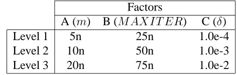
3.7 Levels of the factors used in experimental design . . . 40

3.8 Analysis of variance table for the function Sine Envelope . . . 40

3.9 Analysis of variance table for the function Shekel [S5] . . . 41

4.1 Results for Dixon and Szeg¨o [1975] test functions with the refined algorithm 61 4.2 Results for hard test functions . . . 62

5.1 Results of EM using higher order information for Dixon and Szeg¨o [1975] test functions . . . 65

5.2 Comparison of EM using higher order information with other methods for Dixon and Szeg¨o [1975] test functions . . . 66

5.3 Comparison of EMNCM and downhill simplex method . . . 70

5.4 Comparison of EMASL with SA for general test functions . . . 74

5.5 Comparison of EMASL with SA for Dixon and Szeg¨o [1975] test functions 75 5.6 Parameters for constrained test problems . . . 79

5.7 Comparison of penalty and barrier methods on constrained test problems . . 79

(12)

List of Figures

1.1 Illustration of difficulties in optimizing a nonlinear function. . . 6

2.1 The taxonomy of global optimization methods . . . 11

3.1 Superposition Principle( ~ F i3

= q

3 q

i 4"

0 "

r r

2 ~e

r

i=1;2). . . 27

4.1 An example of premature convergence on one dimensional space . . . 45 4.2 Truncated cone in<

2

. . . 50 4.3 Calculation of the probability for Step 2 in<

2

. . . 52 4.4 Calculation of the lower bound for(T(x))in<

2

. . . 54 4.5 The calculation ofr

in< 2

. . . 56

A.1 Goldstein Price function . . . 100 A.2 The starting position of the particles just after the procedure Initialize. . . . 100 A.3 A new point with better objective value. . . 101 A.4 Points start to attract and repel each other. . . 101 A.5 Optimum is found. Points move toward the current best point . . . 102

(13)

Chapter 1 Introduction

In recent years global optimization has become a rapidly developing field. This is because

global optimization problems arise in diverse application areas. Despite its importance and

the efforts invested so far, the methods for solving global optimization problems are not

satisfactory enough. Therefore, the challenge of determining an absolutely best solution

for a general nonlinear function with many variables and complex attributes attracts the

attention of researchers.

1.1 The Problem Statement

We consider the following global optimization problem:

Given a nonempty setS < n

and a real-valued functionf : S ! <, find at least one

pointx

2S such thatf(x

)f(x)for allx2S.

(14)

Chapter 1. Introduction 2

Following this statement, we denote a global optimization problem1_by

minimize f(x)

subject to x2S;

(1.1)

where f is the objective function and S refers to the feasible region. A vector x

2 S

satisfying f(x

) f(x)for all x 2 S is called a global minimizer of f over S and the

corresponding value off is called a global minimum.

Let kkdenote the Euclidean norm in < n

and let " > 0 be a real number. Then an "

-neighborhood of a pointy2< n

is defined as the open ball

B(y;"),fx2< n

:kx yk<"g: (1.2)

A pointx

2Sis called a local minimizer off overS, if there is an">0such that

f(x

)f(x);8x2B(x

;")\S: (1.3)

Notice that by definition every global minimizer is a local minimizer, but the converse is

not true in general.

Throughout this research, we study a special class of optimization problems with bounded

variables in the form of (1.1) where

S ,fx2< n

j l k

x k

u k

; l k

;u k

2<fork =1;:::;ng. (1.4)

We recall that, whenfis continuous andSis a compact subset of< n

, the existence ofx

is

assured by the Weierstrass theorem of the classical analysis [Taylor and Mann, 1972, Horst

and Tuy, 1993]. Because of the ease of maintaining feasibility, the feasible region defined

in (1.4) has been extensively studied by different classes of global optimization methods.

A rigorous discussion on different methods is given in Chapter 2.

1_{In the rest of the dissertation we deal with minimization problems, since maximization problems can be}

(15)

1.1.1 Importance of Global Optimization

The idea of finding the optimum solution of a problem goes back to the development of

cal-culus and is associated with the names of Newton, Lagrange, and Cauchy. Particularly after

World War II, numerous theoretical and computational methods were proposed for solving

optimization problems. Most of these methods are capable of solving problems that have

relatively simple structure, i.e., problems that include functions of few variables or that

include linear or usually unimodal functions. However, a large variety of problems that

include multimodal nonlinear functions with many variables, arise in different application

areas. Some of these application areas are engineering design, production management,

computational chemistry, product mixture design, environmental pollution management,

parameter estimation, VLSI design, and neural network learning [Floudas, 2000].

There-fore finding the optimum solution of an arbitrary function becomes an important challenge.

In last three decades many researchers from different fields such as Applied

Mathe-matics, Operations Research, Industrial Engineering, Management Science, Computer

Sci-ence, and so on, study global optimization to meet this challenge. This diversity stems from

the fact that global optimization covers a wide range of mathematical optimization

meth-ods. Specifying special properties of the objective function f and/or the feasible region

S in (1.1), leads to a different problem that requires a differenr approach [Pint´er, 1996a,

Floudas, 2000]:

Concave minimization:f is a concave function andSis a convex set.

D.C. programming: f can be represented as difference of two convex

func-tions and S consists of equalities and inequalities that can be represented as

difference of two convex functions.

(16)

Sis a convex set.

Combinatorial optimization: f is defined on discrete points, andS consists of

discrete points.

Network problems: f is an arbitrary function, andS usually consists of linear

or convex equilibrium constraints.

Quadratic global optimization:f is an arbitrary quadratic function, andS

con-sists of linear (or quadratic) equalities and inequalities.

Lipschitz optimization:f is an arbitrary Lipschitz continuous function, andS

consists of inequalities that are represented by Lipschitz continuous functions.

Linear and nonlinear complementarity problems: f is product of two vector

functions, andSis usually a convex set.

Generalized geometric programming problems:f belongs to a special class of

functions called signomials, S consists of equalities and inequalities that are

represented by signomials.

Fractional programming:fis a ratio of two real-valued functions,Sis convex.

Nonlinear programming problems: Usually f belongs to the class of twice

continuously differentiable functions, andSis a compact set.

Multiplicative programming:f is represented as the product of several convex

functions, and S consists of equalities or inequalities that are represented by

convex functions or functions that are product of convex functions.

Seperable programming: f is an arbitrary seperable function, andS is usually

a convex set.

Linear programming: f is a linear function, andS is a convex set defined by

(17)

Other mathematical programming problems including convex programming,

parametric optimization, and stochastic optimization.

A quick glance at the rich literature on global optimization shows its significant growth.

We refer to the book by Floudas [2000] for a representative list of publications and

confer-ence proceedings.

1.1.2 Difficulties In Solving Global Optimization Problems

It is well-known that classical gradient-based methods such as the Quasi-Newton method

[Gill and Murray, 1972, Fletcher and Reeves, 1964], modified steepest descent method

[Armijo, 1996] , or conjugate gradient method [Fletcher and Reeves, 1964] may be trapped

by local optima when the feasible region around the global optimum is not well-conditioned

[Beveridge, 1970]. This is because all standard tools of nonlinear optimization such as

derivatives, gradients, subgradients and the like, can at most determine local minima. In

other words, unless certain restrictive assumptions like convexity, Lipschitz condition, etc.

are satisfied, global minimizers are not only hard to find, but also hard to verify.

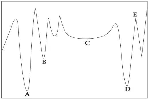
In order to develop efficient methods, it is important to study the difficulties faced by

the classical methods [Shang, 1997]. Let us illustrate some of these difficulties on a

multi-modal nonlinear function in Figure 1.1.

The global minimizer A is in a deep valley and it is surrounded by tall hills

that are difficult to overcome by gradient-based methods.

B is a promising local minimizer that is in the neighborhood of the global

minimizer. A search method may be trapped in B before reaching A.

A search method may spend excessive iterations before passing the shallow

(18)

The promising local minimizer D may mislead the search method to the

re-gions that are far from the global minimizer.

The function is nondifferentiable at E, hence the classical gradient-based

meth-ods can not be applied.

A B

C

D E

Figure 1.1: Illustration of difficulties in optimizing a nonlinear function.

The complexity of solving global optimization problems has been already shown in

a number of theoretical studies. In particular, Murty and Kabadi showed that there exist

quadratic and nonlinear programming problems that belong to the class of NP-complete

problems [1987]. Rinooy Kan and Timmer proved that global optimization problems are

not solvable in finite number of steps [1989]. A similar result has been shown by Pardalos

(19)

1.2 Contributions of This Research

In this dissertation, we introduce a new stochastic global optimization method that is able

to overcome some of the shortcomings of other approaches. We also provide a proof of

convergence to the global optimum for the proposed method.

To be more specific:

The proposed method does not require restrictive assumptions like

differen-tiability, convexity, etc. It works without the higher order information. This

permits us to focus on solving multi-modal, irregular, high dimensional

func-tions, which are difficult to solve by conventional numerical methods.

Like many multi-point methods, the proposed method also works on a set of

sample points (population) of the feasible region and proceeds according to

rel-ative efficiencies of the observed functional values. However, the structure of

the encoding is specifically developed for continuous optimization problems.

Thus, the method can be much faster and the number of function evaluations

can be far less than other methods.

To intensify the search, we use an attraction mechanism between the sample

points rather than partitioning the feasible domain. We add a diversification

effect by using a repulsion mechanism among the points.

Unlike the typical multi-start techniques, the sample points are related to each

other. In other words, the choice of a sample point in successive iterations

depends on the computational experience of the other points in the population.

We compare our results with other global optimization methods. In order to

(20)

flexible, and at the same time, efficient structure. This enables us to elevate

the performance of our approach with additional tools provided by the other

methods.

We prove that the proposed method converges with probability one. The

struc-ture of the proof is flexible and can be generalized for the study of convergence

of other population-based methods.

In constrained optimization problems, the proposed method may be used as a

preprocessing tool for generating feasible points from complicated regions.

The general structure of the proposed method makes it straightforward to

de-velop parallel algorithms.

1.3 Outline of The Dissertation

Current chapter is followed by Chapter 2, which includes a literature survey on different

global optimization methods. The pros and cons of these methods are also discussed in

Chapter 2.

Chapter 3 begins with the motivation behind the proposed method and continues with

the description of the essential procedures. After the presentation of the proposed method,

computational results on different problems are given. Chapter 3 ends with an experiments

section that explains the effects of different parameters.

In Chapter 4, we show the convergence properties of the proposed method. In order

to achieve the desired result, several procedures are modified. Then it is shown that the

proposed method converges with probability one. The chapter ends with a discussion on

(21)

Several variants of the proposed method along with some extensions are given in

Chap-ter 5. Each variant is tested on a set of problems and then compared with some other

methods. Chapter 5 also covers a preliminary study regarding constrained optimization

problems.

We conclude the dissertation with Chapter 6. In addition to giving an overview of

the dissertation, we discuss further research areas in a seperate section. The appendices

contain an example run of the proposed method and the test functions used throughout the

(22)

Chapter 2 Literature Review

Dixon and Szeg¨o published one of the earliest collection of papers devoted to global

op-timization [1975, 1978]. In light of this pioneering work, considerable variety of global

optimization models and solution approaches have been studied. Here, we give a brief

review of the global optimization literature.

2.1 Taxonomy of Global Optimization Methods

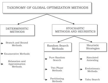
In the field of global optimization, it is quite common to classify the methods into two

main categories: deterministic methods and stochastic (or probabilistic) methods [T¨orn

and Zilinskas, 1989, Horst and Pardalos, 1995]. As the names imply, the methods that do

not involve random elements go into the former category, whereas the methods that utilize

probabilistic schemes go into the latter category. We remark that for many global

optimiza-tion methods, the distincoptimiza-tion between deterministic and stochastic is blurred. There are

very effective methods, which involve deterministic as well as stochastic elements.

In recent years, with the increase in computer speed, a third category - heuristics - has

(23)

Chapter 2. Literature Review 11

emerged. Many of these heuristic strategies involve stochastic elements. Hence we extend

the stochastic methods category to include the heuristic methods.

This review consists of two parts: The first part presents the deterministic global

opti-mization methods. The second part gives a comprehensive treatment of stochastic methods

and heuristics - in which our proposed method also appears. Beyond our discussion, many

additional references for specific approaches can be found within the cited literature.

Figure 2.1 gives the taxonomy for global optimization methods that we shall follow in

our review.

(24)

2.2 Deterministic Methods

In this section, we introduce some of the deterministic global optimization methods. The

methods discussed in this section are direct methods, for which strong theoretical

conver-gence results can be proven under certain assumptions. Most of these methods are

de-veloped for special classes of problems. Hence their performances may deteriorate with

different problem classes. In addition, a method with a global convergence property may

be so complicated that it may be intractable from a practical point of view.

Surveys and monographs which provide general coverage of deterministic methods

in-clude Dixon and Szeg¨o [1975], Neumaier [1990], Floudas and Pardalos [1992], Horst and

Tuy [1993], Kearfott [1996], Pint´er [1996b], Floudas [2000], and Horst et al. [2000].

Branch and Bound Methods

Branch and bound methods are based on the idea of decomposing the original problem into

smaller subproblems (branches) that are easier to handle. The same process is applied to

the subproblems, and this process goes on until the optimal solution of any subproblem

pro-vides an optimal solution to the original problem. Nevertheless, as the number of branches

increases, the number of subproblems grows exponentially. Hence, it becomes crucial to

eliminate some of the subproblems. This requires a bounding scheme, which is based on

setting lower bounds on the optimal objective function values of the subproblems.

Initially, branch and bound methods were developed for integer programming

prob-lems, where the exhaustive search feature of the methods guarantees the global

conver-gence [Nemhauser and Wolsey, 1988]. Recently, branch and bound methodology has been

(25)

Pardalos and Rosen [1986] give a survey on the applications of branch and bound methods

to solve general concave minimization problems.

Branch and bound methods are also applied to continuous global optimization

prob-lems, where the exhaustive enumeration concept is replaced by a global convergence

ar-gument [Horst and Tuy, 1987, Pint´er, 1992, Csendes and Pint´er, 1993, Kearfott, 1996].

Lipschitz optimization and interval methods are two effective approaches along this line

[Ratschek and Rokne, 1995, Hansen and Jaumard, 1995]. These methods are extensively

used for solving real world applications [Pint´er, 1996b]. Nevertheless, both methods

re-quire a priori knowledge relative to the structure of the problem. In Lipschitz optimization,

it is assumed that the modeler knows suitable constants (namely Lipschitz constants), which

show how rapidly each function vary [Armijo, 1996, Pint´er, 1996b]. In interval methods

the functions are required to satisfy certain smoothness properties [Neumaier, 1990, Ratz

and Csendes, 1995, Kearfott, 1996].

Enumerative Methods

In particular cases, a global optimization problem may have finite number of local

mini-mizers. Enumerative methods try to find all these minimizers in order to locate the global

minimizer. This seemingly “elementary” idea is supported by rigorous theoretical results

and many successful implementations [Watson and Yang, 1980, Diener, 1986].

Path-following (or trajectory) methods rely on constructing a set of paths (or

trajecto-ries) such that all solutions of the problem are known a priori to lie on one of these paths. In

many cases, these paths are derived from solving a system of differential equations.

Start-ing from an initial point, the solutions along these paths are usually found by a numerical

(26)

Homotopy (or parameter continuation) methods are similar to path-following methods.

Homotopy methods work by first solving a simple problem and then parametrically

trans-forming this problem into the original problem. This transformation leads to the concept

of homotopies, which are used for generating the set of paths. After finding the paths to be

traced, this approach can be extended to search for all solutions of the problem [Garcia and

Zangwill, 1981, Forster, 1995].

The main drawback of the path-following and homotopy methods is the lack of a

guar-antee of generating all the paths leading to the solutions. Another restriction common to

these methods is the requirement that the functions to be twice continuously differentiable.

Relaxation and Approximation Methods

The history of relaxation and approximation methods preceedes the introduction of global

optimization as a seperate field. In particular, these methods were used for solving difficult

combinatorial optimization problems [Nemhauser and Wolsey, 1988].

The essential idea in relaxation and approximation methods is to solve a sequence of

simple subproblems, which are derived from the original problem by successive

relax-ations. Then, these subproblems are extended by adding constraints such that the original

problem is more closely approximated [Horst and Tuy, 1993, Horst and Pardalos, 1995].

A very important approach among these methods is the cutting plane method [Kelley,

1960, Westerlund and Pettersson, 1995]. The basic idea of the cutting plane method is to

iteratively cut off parts of the feasible region that does not include the global minimizer.

Then the search for the solution of the problem continues in the remaining part of the

feasible region. It has been shown that cutting plane methods are useful for diverse global

(27)

(D.C.) and reverse convex problems [Tuy, 1987b,a, Thoai, 1988].

There are different difficulties that may arise with relaxation and approximation

meth-ods. Mainly, the subproblems derived from the original problem can still be complex. In

this case, a further relaxation may cause too much oversimplification of the original

prob-lem. Furthermore, adding a constraint at each iteration may complicate the subproblems so

that an efficient constraint dropping strategy may become necessary.

2.3 Stochastic Methods and Heuristics

This section covers global optimization methods that are mostly based on random sampling

from the feasible region. Some of these stochastic methods converge (with probability

one) to the global minimizer. We also review some of the heuristic strategies, which are

motivated by certain analogies with natural phenomena or basic sciences. In many cases,

these heuristics provide usable solutions even when deterministic methods fail because of

the irregularities or high dimensionality. However, for most of the heuristics a rigorous

treatment of global convergence properties does not exist.

For a general coverage of different stochastic methods and heuristics, see Dixon and

Szeg¨o [1978], Pint´er [1984], Boender et al. [1985], Rinooy Kan and Timmer [1987a,

1987b], Laarhoven and Aarts [1987], T¨orn and Zilinskas [1989], Goldberg [1989],

Zim-mermann [1990], Zhigljavsky [1991], Kosko [1993], Rinooy Kan and Timmer [1994],

Boender and Romeijn [1995], Osman and Kelly [1996] , Aarts and Lenstra [1997], and

(28)

2.3.1 Random Search Methods

Random search methods constitute the core element of many complex stochastic global

optimization methods. In this section, we try to include the methods that have played a

pioneering role in the development of many other stochastic methods.

Pure Random Search

Pure random search is the simplest stochastic method for solving global optimization

prob-lems. Main idea is to sample a sequence of independent identically distributed random

points from the feasible region, while keeping the track of the best objective function value

achieved [Brooks, 1958, Anderssen and Bloomfield, 1975, Zhigljavsky, 1991, Zabinsky

and Smith, 1992]. In this case, the proof of convergence to the global optimum (with

prob-ability one) can be easily shown [Baba et al., 1977, Devroye, 1978, Baba, 1981, Solis and

Wets, 1981, Pint´er, 1984].

In general, pure random methods are easy to implement. Therefore, they are often used

as a first approach to solve complex problems. Moreover, in many cases these methods

are modified leading to more complicated algorithms [Smith, 1984, Berbee et al., 1987].

However, pure random search methods are not efficient, especially for problems with higher

dimensions, since in this case the number of iterations required to solve a problem increases

fast.

Two-Phase Methods

In two-phase methods, the search is divided into two steps. In the global phase, the function

is evaluated at a number of randomly sampled points, while in the local phase, the sample

(29)

[Rinooy Kan and Timmer, 1987a, Boender and Romeijn, 1995].

Density Clustering, Controlled Random Search, Multistart, and the Multi Level Single

Linkage (MLSL) [Rinooy Kan and Timmer, 1994] are well-known two-phase methods that

enable the exploration of the whole feasible region through random sampling followed by

hill-climbing or gradient-based methods. In spite of a few successful results [Boender et al.,

1985], there are numerous cases when these methods are inefficient. The main reason for

this is that they inevitably cause each local minimum to be visited several times [Dekkers

and Aarts, 1991].

Topographical MLSL (TMLSL) [Ali and Storey, 1994] and Topographical

Optimiza-tion with Local Search (TOLS) [T¨orn and Viitanen, 1994] are two more recently developed

methods of this type. TMLSL and TOLS are both reported to be considerably superior to

MLSL and other previously introduced clustering methods. Nevertheless, these methods

may fail in two different ways. First, the resulting groups of points, or clusters, may

con-tain several regions of attractions, so that the global minimum can be missed. Second, one

region of attraction may be divided over several clusters, in which case the corresponding

optimum will be located more than once [Rinooy Kan and Timmer, 1987a].

Partitioning Methods

Partitioning schemes, which divide the feasible region into smaller subspaces, discard some

unfavorable regions, and re-partition promising areas to reduce the final search space, have

also been proposed for global optimization [Jones et al., 1993, Wood, 1991, Caprani and

Madsen, 1993].

Recently, Demirhan et al. proposed a partitioning algorithm, with a fuzzy region

(30)

literature [Anroulakis and Vrahatis, 1996, Michalewicz, 1994, Srinivas and Patnaik, 1994].

Difficulties arise when the function has attractive regions spread around the feasible

space. In this case, partitioning methods may discard an area which actually includes the

global optimum. In addition, in most cases an extensive number of function evaluations is

inevitable.

2.3.2 Heuristic Strategies

Starting in the 1980’s, a wide range of novel approaches, which rely heavily on computer

speed, have been developed. Some of these methods are inspired by careful observations

of natural phenomena and some of them are developed merely by implementing practical

ideas.

Simulated Annealing

Simulated Annealing (SA) is a stochastic single-point search technique, which has been

applied successfully in various optimization fields. SA guides the search by specifying a

cooling scheme that allows the acceptance of randomly generated neighbor solutions which

are relatively unfavorable as compared with the current solution [Kirkpatrick et al., 1983,

Laarhoven and Aarts, 1987]. Using the latter feature, SA aims to escape entrapment at

local optima. The temperature described by the cooling scheme is reduced as the search

makes progress so that the search is intensified around the global optimum. There exist

different convergence proofs for the variants of SA [Dekkers and Aarts, 1991, Boender

and Romeijn, 1995]. The strong points of SA and some pitfalls for potential SA users are

indicated in an extensive review given by Ingber [1994], where a wide range of application

(31)

a multi-start search technique is also discussed in the same paper.

In spite of the successful results reported for SA [Kirkpatrick et al., 1983, Aarts and

Korst, 1997], a serious deficiency in the method is that the results depend on the starting

point of each run. Furthermore, any combination with a multi-start technique and/or

ap-plication of parallelization techniques increases the computational effort drastically [Birbil

et al., 1999, ¨Ozdamar and Demirhan, 2000].

Evolutionary Methods

Although initially described as classifier systems and reflections of evolutionary systems,

Genetic Algorithms (GA) have recently become popular global optimization techniques,

specifically in combinatorial optimization [Goldberg, 1989]. GAs investigate the feasible

space by utilizing populations of solutions, which evolve by reproduction, crossover, and

mutation operators [Michalewicz, 1994].

An interesting method using GA operators is provided by Wodrich and Bilchev [Wodrich

and Bilchev, 1997]. The authors use crossover and mutation operators to create new

re-gions of search for the Ant Colonization technique originally proposed for the Traveling

Salesman Problem by Dorigo and Colorni [Dorigo and Colorni, 1996]. In their case, all

of numerical results are for combinatorial optimization problems. To our knowledge, all

the implementations of Ant Colonization technique have been for discrete optimization

problems. Nevertheless, it is reasonable to expect new implementations for continuous

optimization inspired by the discrete counterparts.

Although they provide powerful optimization tools for difficult optimization problems

[Schaffer, 1989, Birbil, 1999], a serious handicap of evolutionary methods is the heavy

(32)

addition, the structure of the encoding used in these methods is not usually adequate for the

continuous global optimization problems.

Tabu Search

The first influential work on tabu search was published in late 1980’s by Glover [1986].

After this pioneering result, additional efforts on formalization [Glover, 1989, 1990] and a

monograph for a complete discussion were presented [Glover and Laguna, 1997].

Further-more, a recent work by Glover et al. showed that tabu search is a flexible approach that can

be merged with other methods [1995].

Tabu search is an iterative scheme, which is based on moving from one point to a

neighborhood point in single iteration. Throughout this search, main idea is to keep track of

not only the local information but also some information related to the exploration process.

This scheme requires a systematic handling of (tabu) lists, which hold the history of moves

and prevents them to be revisited.

Though no rigorous convergence proof has been shown, many successful applications

of tabu search are reported [Glover and Laguna, 1997]. However, the successful

appli-cations are given only for combinatorial optimization problems and the appliappli-cations for

continuous global optimization problems are in their early stages of development [Battiti

and Tecchiolli, 1996].

2.4 Other Work

Before describing our proposed approach, we cite several references we used in our

(33)

and Neumaier [1999]. The proposed algorithm has powerful theoretical convergence

prop-erties. However, for unconstrained problems in four dimensional space or above, the

perfor-mance of MCS is less satisfactory than for small problems. Huyer and Neumaier compare

MCS with existing approaches on different test problems. We make use of their work to

compare our proposed method with other approaches.

In a recent survey, T¨orn et. al. [T¨orn et al., 1999] study the characteristics of

uncon-strained global optimization test problems. They classify the problems as unimodal, easy,

moderately difficult and difficult problems. The features considered in this classification

are the chance of missing the region of attraction of the global minimum, embededness of

the global minimum, and the number of local minimizers. An example of a representative

set of test problems is also discussed. In our numerical work, we test our algorithm with

some of the problems from their paper.

Following our joint report [Birbil et al., 1999], ¨Ozdamar and Demirhan developed

sev-eral heuristic strategies for solving 77 small to moderate size (up to 10 variables) nonlinear

test functions and 18 large size test functions (up to 400 variables) collected from literature

[2000]. In Chapter 5, we compare a variant of our proposed method with one of the most

successful approaches that ¨Ozdamar and Demirhan reported.

To test the extended version of our method, we selected several constrained problems

from the book by Floudas and Pardalos [1990] who collected a large set of test problems

arising in the literature and in a wide range of applications [1990]. These test problems are

available at a web site [Floudas et al., 2002].

Neumaier has developed an excellent web site for global optimization [2002]. Like

many researchers, we have reached to other useful links through his site. In particular, the

(34)

Chapter 3 Electromagnetism-like Mechanism (EM)

In stochastic global optimization, population-based algorithms start with randomly

sam-pling points from the feasible region. According to the objective function values of these

sample points, the regions of attraction are determined. Then a mechanism is invoked for

further exploitation of these candidate regions. In GAs this mechanism corresponds to the

reproduction, crossover and mutation operators [Michalewicz, 1994], whereas in two phase

methods the exploration of the feasible region is conducted by random sampling followed

by hill-climbing [Rinooy Kan and Timmer, 1987a, T¨orn and Viitanen, 1994] or

gradient-based methods [Fletcher and Reeves, 1964].

Similarly, we construct a mechanism that encourages the points to converge to the

highly attractive valleys, and contrarily, discourages the points to move further away from

steeper hills. This idea enables us to make an analogy with the attraction-repulsion

mech-anism of the electromagnetism theory [Birbil and Fang, 2000a,b].

Under this analogy, we can think of each sample point as a charged particle that is

released to a space. In our approach, the charge of each point relates to the objective

function value, which we are trying to optimize. This charge also determines the magnitude

(35)

Chapter 3. Electromagnetism-like Mechanism (EM) 23

of attraction or repulsion of the point over the sample population - the better the objective

function value, the higher the magnitude of attraction.

After calculating these charges, we use them to find a direction for each point to move

in subsequent iterations. We select this direction by evaluating a combination force exerted

on the point via other points. Like the electromagnetic forces, this force is calculated by

adding vectorially the forces from each of the other points calculated separately.

We need to state that though the analogy with electromagnetism theory motivates the

idea, there are some notable differences that we make clear when we introduce the method

in the subsequent sections.

Finally, similar to the hybrid population-based algorithms [Hart, 1994, Glover et al.,

1995], we may apply a local search procedure to improve some of the objective function

values observed in the population. In the rest of this chapter, we introduce this new method

and present the algorithmic structure. This is followed by the presentation of the numerical

results.

3.1 General Scheme for EM

We deal with the problems of the form (1.1) withS defined as in (1.4). Thus, we assume

that the following are known from the problem:

n: dimension of the problem.

u

k: upper bound in the k

th

dimension.

l

k: lower bound in the k

th

dimension.

(36)

The proposed method EM consists of four phases: initialization of the sample points,

calculation of the total force exerted on each particle 1_{, movement along the direction of}

the force, and application of neighborhood search to exploit the local minima. The general

scheme is given in Algorithm 1. The parameters are explained in the following

subsec-tions, when we thoroughly describe each part of the general scheme with accompanying

algorithms.

Algorithm 1 EM(m,MAXITER,LSITER,Æ)

m: number of sample points

MAXITER: maximum number of iterations

LSITER: maximum number of local search iterations Æ: local search parameter, Æ2[0;1]

1: Initialize()

2: iteration 1

3: whileiteration<MAXITERdo

4: Local(LSITER,Æ)

5: F CalcF()

6: Move(F)

7: iteration iteration+1

8: end while

3.1.1 Initialization

The procedure Initialize is used to sample m points randomly from the feasible domain,

which is an n dimensional hyper-cube. Each coordinate of a point is assumed to be

uni-formly distributed between the corresponding upper bound and lower bound. After a point

is sampled from the feasible region, the objective function value for the point is calculated

using the function pointerf(x)(Algorithm 2, line 6). The procedure ends withm points

identified, and the point that has the best function value stored inx best

(line 8).

(37)

Algorithm 2 Initialize()

1: fori=1tomdo

2: fork =1tondo

3: U (0;1)

4: x

i k

l k

+(u k

l k

)

5: end for 6: Calculatef(x

i )

7: end for 8: x

best

argminff(x i

);8ig

3.1.2 Local Search

The procedure Local is used to gather the local information for a pointx i

. The parameters,

LSITER andÆ that are passed to this procedure, represent the number of iterations and the

multiplier for the neighborhood search, respectively.

The procedure iterates as follows: First, the maximum feasible step length (Length) is

calculated by using the parameterÆ (Algorithm 3, line 2). Second, for a giveni,

improve-ment in x i

is sought coordinate by coordinate (lines 5-13). For a given coordinate, the

pointx i

is assigned to a temporary pointyto store the initial information. Next, a random

number is selected as a step length and the point y is moved along that direction. If the

pointyobserves a better point within LSITER iterations, the pointx i

is replaced byyand

the neighborhood search for point i ends (lines 14-17). Finally the current best point is

updated (line 22).

This is a simple random line search algorithm applied coordinate by coordinate. This

procedure does not require any gradient information to perform the local search. Instead

of using other powerful local search methods, we have utilized this procedure because we

wanted to show that even with this trivial method, the algorithm shows promising

(38)

Algorithm 3 Local(LSITER,Æ)

1: counter 1

2: Length Æ(max k

fu k

l k

g)

3: fori=1tomdo

4: fork =1tondo

5:

1

U (0;1)

6: whilecounter<LSITERdo

7: y x

i

8:

2

U (0;1)

9: if

1

>0:5then

10: y

k y

k +

2

(Length)

11: else

12: y

k y

k

2

(Length)

13: end if

14: iff(y)<f(x i

)then

15: x

i y

16: counter LSITER 1

17: end if

18: counter counter+1

19: end while 20: end for 21: end for 22: x

best

argminff(x i

(39)

3.1.3 Calculation of Total Force Vector

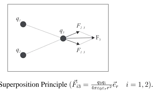
The superposition principle of electromagnetism theory states that the force exerted on

a point via other points is inversely proportional to the distance between the points and

directly proportional to the product of their charges [Cowan, 1968].

q1

q2

q3 F2 3

F1 3

F3

Figure 3.1: Superposition Principle( ~ F i3

= q3qi 4"0"rr

2 ~e

r

i=1;2).

Analogously, in each iteration we determine the charge of every point according to the

objective function values of the points. However, in our method the charge of each point is

not constant and changes from iteration to iteration.

The charge of each point,q i

determines pointi’s power of attraction or repulsion. This

charge is evaluated by

q i

=exp( n

f(x i

) f(x best

) P

m k=1

(f(x k

) f(x best

))

); 8i: (3.1)

In this way, points that have better objective values possess higher charges. We multiply

the fraction by the dimensionn, because in higher dimensions the number of points in the

population tends to get large. As a result of this, the fraction may become very small, and

may cause overflow problems in calculating the exponential function.

We define the charge, q i

(40)

value of the corresponding point in the population. This is clearly not the unique nor

the optimal choice for this calculation. An alternative calculation, which rank the points

according to their objective function values, may be used here. Our experiments have

shown that the proposed calculation in Equation (3.1) is satisfactory for our study.

Notice that, unlike electrical charges, no signs are attached to the charge of an individual

point in Equation (3.1). Instead, we decide the direction of a particular force between two

points after comparing their objective function values. Hence, the total forceF i

exerted on

pointiis computed by the following:

F i = m X j6=i 8 > < > : (x j x i ) q i q j kx j x i k 2

if f(x j

)<f(x i ) (x i x j ) q i q j kx j x i k 2

if f(x j

)f(x i ) 9 > = > ;

;8i (3.2)

Algorithm 4 CalcF():F

1: fori=1tomdo

2: q i exp( n f(x i ) f(x best ) P m k =1 (f(x k ) f(x best )) ) 3: F i 0

4: end for

5: fori=1tomdo

6: forj =1tomdo

7: iff(x j

)<f(x i )then 8: F i F i +(x j x i ) q i q j k x j x i k 2

fAttractiong

9: else 10: F i F i (x j x i ) q i q j kx j x i k 2

fRepulsiong

11: end if 12: end for 13: end for

As seen in Algorithm 4 (lines 7-8), between two points, the point that has a better

ob-jective function value attracts the other one. Contrarily, the point with worse obob-jective

function value repels the other (lines 9-10). Since x best

has the minimum objective

(41)

population.

When we examine the algorithm carefully, we can see that the determination of a

direc-tion via total force vector resembles the statistical estimadirec-tion of the gradient off. However,

the estimation computed by our method is different since this direction depends on the

Eu-clidean distance between the points. That is, the points that become close enough may lead

each other to a direction other than the statistically estimated one.

3.1.4 Movement According to Total Force Vector

After evaluating the total force vectorF i

, the pointiis moved in the direction of the force

by a random step length as given in Equation (3.3). Here the random step length, , is

assumed to be uniformly distributed between 0 and 1. Obviously, there are many other

distributions that can be used in calculation of this step length. But for ease of computation,

we have applied uniform distribution. We have selected the step length randomly in order

to ensure that the points have a nonzero probability to move to the unvisited regions along

this direction.

In Equation (3.3), R NG is a vector whose components denote the allowed feasible

movement toward the upper bound, u k

, or the lower bound, l k

, for the corresponding

di-mension (Algorithm 5, lines 6-10). Furthermore, the force exerted on each particle is

nor-malized so that we can maintain the feasibility. Thus,

x i

=x i

+ F

i

kF i

k

(R NG) i=1;2;:::;m: (3.3)

Algorithm 5 gives the Move procedure. Note that the best point,x best

, is not moved and

is carried to the subsequent iterations (line 2). This suggests that we may avoid the

(42)

effort for calculating the total force vector on a single point is negligible).

Algorithm 5 Move(F)

1: fori=1tomdo

2: ifi6=bestthen

3: U (0;1)

4: F i F i k F i k

5: fork =1tondo

6: ifF

i k

>0then

7: x i k x i k +F i k (u k x i k ) 8: else 9: x i k x i k +F i k (x i k l k )

10: end if 11: end for 12: end if 13: end for

3.1.5 Termination Criteria

In our study we terminate EM by using a maximum number of iterations. According to our

test results, in general 25 iterations per dimension (i.e.,MAXITER =25n) is satisfactory

for solving the moderate difficulty functions.

Another termination criterion that might be used is the successive number of iterations

spent without changing the current best point. In other words, if the current best point is

not changed for certain number of iterations, the algorithm may be stopped. However this

decision has to be studied carefully since algorithm may be terminated before converging to

the global optimum. On the other hand, unnecessary function evaluations may be avoided

by stopping earlier.

In the literature several other stopping conditions are studied [Boender and Romeijn,

(43)

when the observed objective function value is "-close to the optimal value [Huyer and

Neumaier, 1999]. However, this criterion is not appropriate if the global optimum is not

known in advance.

3.2 Computational Results

In a recent paper, T¨orn et al. classified the well-known global optimization problems as

unimodal, easy, moderately difficult, and difficult problems [1999]. They also suggested

that the test problems should represent different classes. We have included some of the

functions that T¨orn et al. discussed and we have created a test function set consisting of 15

functions. We refer to this test function set as the general test functions. The functions and

their references are given in Appendix B.1.

Initially, we studied three versions of EM, which differ in the local search procedure.

We demonstrate our results for the general test functions in terms of the average number

of function evaluations over 25 runs. The average and best objective function values are

also reported. After selecting the best version, we applied EM to a well known test set,

which consists of seven test functions [Dixon and Szeg¨o, 1975]. In addition to reporting

our results, we compare the results with other methods reported by Huyer and Neumaier

[1999].

All the computations were conducted on a Pentium-III 450 MHz PC. The algorithm has

(44)

3.2.1 General Test Functions

We tested EM with three different versions of the Local procedure. First, we excluded the

local procedure completely from the general scheme. Second, we applied the procedure to

all sample points. Finally, we utilized the local search procedure with the best point only.

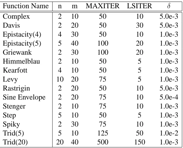
The input parameters for the functions are given in Table 3.1. The functions are

pre-sented in alphabetical order, so the order of a function does not necessarily represent the

difficulty of the corresponding function.

Table 3.1: Parameters for General Test Functions

Function Name n m MAXITER LSITER Æ

Complex 2 10 50 10 5.0e-3

Davis 2 20 50 30 5.0e-3

Epistacity(4) 4 30 50 10 1.0e-3

Epistacity(5) 5 40 100 20 1.0e-3

Griewank 2 30 100 20 1.0e-3

Himmelblau 2 10 50 5 1.0e-3

Kearfott 4 10 50 5 1.0e-3

Levy 10 20 75 5 1.0e-3

Rastrigin 2 20 50 10 5.0e-3

Sine Envelope 2 20 75 10 5.0e-4

Stenger 2 10 75 10 1.0e-3

Step 5 10 50 5 1.0e-3

Spiky 2 30 75 10 1.0e-3

Trid(5) 5 10 125 50 1.0e-2

Trid(20) 20 40 500 150 1.0e-3

EM without Local procedure

In order to examine the basic convergence properties of EM, we first excluded the Local

(45)

Table 3.2: Results of EM without Local procedure

Function Name Avg. Evals. Avgf(x) Bestf(x) Known Optimum

Complex 363 0.0175 0.0158 0.0

Davis 622 1.6157 1.5641 0.0

Epistacity(4) 1079 0.0379 0.0149 0.0

Epistacity(5) 2603 0.0355 0.0207 0.0

Griewank 1914 0.0896 0.0032 0.0

Himmelblau 84 0.0934 0.0759 0.0

Kearfott 231 0.0008 0.0000 0.0

Levy 835 0.1429 0.0303 0.0

Rastrigin 141 -1.9566 -1.9871 -2.0

Sine Envelope 962 0.0744 0.0400 0.0

Stenger 282 0.0020 0.0019 0.0

Step 728 0.0000 0.0000 0.0

Spiky 1702 -38.6378 -38.7251 -38.85

Trid(5) 968 -28.2997 -29.0324 -30.0

Trid(20) 43354 -33.2567 -177.6124 -1520.0

to 0. The immediate effect of this choice is the loss of the local information. In this case,

even when a point is close to a local optimizer, it is not directed deeper into the valley. In

certain sense, this approach behaves blindly. However, since no additional information is

collected, the average number of function evaluation figures are not large.

The results in Table 3.2 show that the solutions for the functions Davis and Trid(20) are

less satisfactory than those for the other functions. Davis is highly irregular in the

neighbor-hood of the optimum, while the feasible region of Trid(20) is a 20-dimensional hypercube

with bounds [ 400;400] in each dimension. Therefore the number of evaluations in an

experiment is not large enough to adequately explore the feasible space.

Our results show that even if we do not use the Local procedure, the average function

(46)

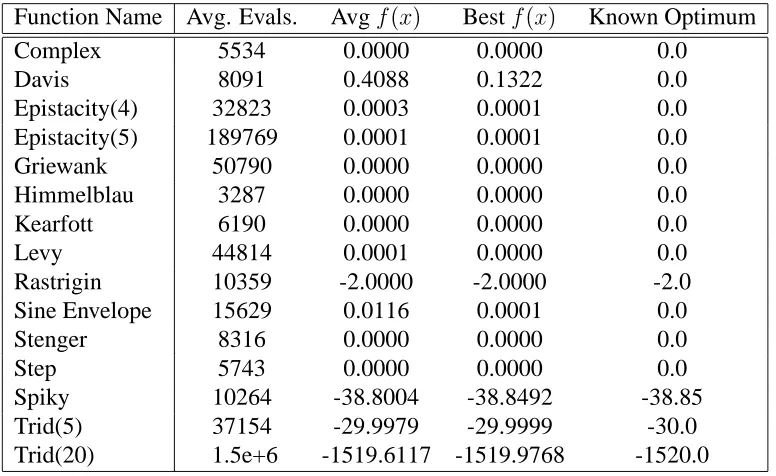
Table 3.3: Results of EM with Local procedure applied to all points

Complex 5534 0.0000 0.0000 0.0

Davis 8091 0.4088 0.1322 0.0

Epistacity(4) 32823 0.0003 0.0001 0.0

Epistacity(5) 189769 0.0001 0.0001 0.0

Griewank 50790 0.0000 0.0000 0.0

Himmelblau 3287 0.0000 0.0000 0.0

Kearfott 6190 0.0000 0.0000 0.0

Levy 44814 0.0001 0.0000 0.0

Rastrigin 10359 -2.0000 -2.0000 -2.0

Sine Envelope 15629 0.0116 0.0001 0.0

Stenger 8316 0.0000 0.0000 0.0

Step 5743 0.0000 0.0000 0.0

Spiky 10264 -38.8004 -38.8492 -38.85

Trid(5) 37154 -29.9979 -29.9999 -30.0

Trid(20) 1.5e+6 -1519.6117 -1519.9768 -1520.0

Nevertheless, the average objective function value figures show that in some cases, EM

did not converge to the global optimum, and the accuracy of the objective function values

degraded. This motivated the next experiment.

EM with Local procedure applied to all points

We next applied the Local procedure to all points in the population. This approach has

two advantages; first, the attractive parts of the feasible region are more thoroughly

ex-amined, and second, the repelled points have better chance to lead to as yet undiscovered

minimizers.

Notice that the performance of the algorithm improves but at the cost of the number of

(47)

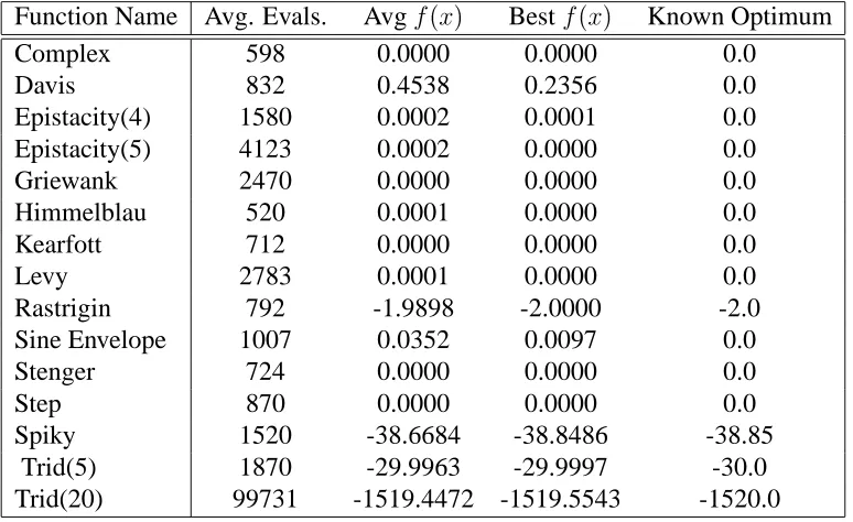
Table 3.4: Results of EM with Local procedure applied to current best point

Complex 598 0.0000 0.0000 0.0

Davis 832 0.4538 0.2356 0.0

Epistacity(4) 1580 0.0002 0.0001 0.0

Epistacity(5) 4123 0.0002 0.0000 0.0

Griewank 2470 0.0000 0.0000 0.0

Himmelblau 520 0.0001 0.0000 0.0

Kearfott 712 0.0000 0.0000 0.0

Levy 2783 0.0001 0.0000 0.0

Rastrigin 792 -1.9898 -2.0000 -2.0

Sine Envelope 1007 0.0352 0.0097 0.0

Stenger 724 0.0000 0.0000 0.0

Step 870 0.0000 0.0000 0.0

Spiky 1520 -38.6684 -38.8486 -38.85

Trid(5) 1870 -29.9963 -29.9997 -30.0

Trid(20) 99731 -1519.4472 -1519.5543 -1520.0

of the results for the functions Davis, Levy, and Trid(20) are much better. However, the

number of evaluations drastically increases for the problems with high dimensionality.

EM with Local procedure applied to the current best point only

To reduce the number of function evaluations, we tried applying Local procedure to the

current best point only (Table 3.4). This choice balances the number of evaluations and the

accuracy of the results.

In this case, the average number of evaluations is closer to those of the first version

(without Local procedure), while the quality of the results is comparable to those of the

second version (Local procedure applied to all points ). However, when the function has

(48)

Table 3.5: Results of EM for Dixon and Szeg¨o [1975] test functions

Function [(a)] n m MAXITER Avg. Evals. Avgf(x) Bestf(x) f glob

Shekel [S5] (b) 4 40 150 3368 -9.7320 -10.1532 -10.1532 Shekel [S7] 4 40 150 1782 -10.4024 -10.4029 -10.4029 Shekel [S10] 4 40 150 5620 -10.5109 -10.5109 -10.5364

Hartman [H3] 3 30 75 1114 -3.8625 -3.8628 -3.8628

Hartman [H6] 6 30 75 2341 -3.3072 -3.3224 -3.3224

Goldstein Price [GP] 2 20 50 420 3.0001 3.0000 3.0000

Branin [BR] 2 20 50 315 0.3980 0.3979 0.3979

Six Hump Camel [C6] 2 20 50 233 -1.0316 -1.0316 -1.0316 Shubert [SHU] 2 20 50 358 -186.7227 -186.7309 -186.7309 (a) : The labels of the functions are given in brackets [Huyer and Neumaier, 1999].

(b) : 2 of the 25 runs do not converge to the global optimum.

the points visiting the neighborhood of the global optimum may not be powerful enough to

attract other points. In function Davis, the algorithm rapidly converges to the neighborhood

of the optimum point, but the region around global optimum has many local minimizers in

steep valleys. Thus, EM is trapped in one of these local minima.

3.2.2 Dixon and Szeg¨o Test Functions

Our initial experiments show that EM rapidly converges to the minimizers. The local

infor-mation gains more importance either when the function is highly irregular in the

neighbor-hood of the global optimum, or when the global optimum is far from the highly attractive

local minimizers. Although the application of the local search to all points provides the

best results, the improvement over applying local search only to the current best point is

not significant. Therefore, for most of the problems, applying local search to all points may

turn out to be overkill. In the subsequent experimentation, we utilized the third version of

EM for comparison with other global optimization methods.

(49)

[1975]. The performance of different methods on these functions has been extensively

studied by Huyer and Neumaier [1999]. We use their results in comparing EM with the

existing approaches. As a stopping criterion we use the following Equation (3.4), that is

also applied by Huyer and Neumaier [1999]:

(f(x best

) f gl ob

) jf

gl ob j

10 4

(3.4)

wheref

gl ob represents the known global optimum.

Table 3.5 shows our results with the corresponding parameters. EM does not exhibit

any difficulty to converge to the global optimum in all functions, except Shekel [S5]. This

function has an attractive local minimizer, which is far from the global optimum.

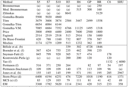
Table 3.6 shows the comparison of EM with other methods in terms of number of

function evaluations. Except for the last row, the figures in the table are taken from [Huyer

and Neumaier, 1999]. From the table we see that MCS achieves the best results followed

generally speaking by the other methods (labeled with (f) and (h)), which use first or second

order information in the neighborhood search. EM does as well as or better than the most

of the older methods indicated in the upper part of the table.

Overall, our additional comments are in order:

Unlike MCS and other methods indicated with (f), EM does not use the first or

the second order information.

EM is able to provide answers for all the problems.

All the methods, other than EM that are included in Table 3.6, have some

limitations due to their rigid structures. EM has a very flexible design which

would permit using the desirable features from other methods.

(50)

Table 3.6: Comparison of EM with different methods in terms of number of function

evaluations

Method S5 S7 S10 H3 H6 GP BR C6 SHU

Bremmerman (a) (a) (a) (a) (a) (a) 250

Mod. Bremmerman (a) (a) (a) (a) 515 300 160

Zilinskas (a) (a) (a) 8641 5129

Gomulka-Branin 5500 5020 4860

T¨orn 3679 3606 3874 2584 3447 2499 1558

Gomulka-T¨orn 6654 6084 6144

Gomulka-V.M. 7085 6684 7352 6766 11125 1495 1318

Price 3800 4900 4400 2400 7600 2500 1800

Fagiuoli 2514 2519 2518 513 2916 158 1600 De Biase-Frontini 620 788 1160 732 807 378 587

Mockus 1174 1279 1209 513 1232 362 189

B´elisle et al. (b) 339 302 4728 1846

Boender et al. (f) 567 624 755 235 462 398 235

Snyman-Fatti (f) 845 799 920 365 517 474 178

Kostrowicki-Piela (g) (c) (c) (c) 200 200 120 120

Yao (f) 1132 6000

Perttunen (f) 516 371 250 264 82 97 54 197

Perttunen-Stuckman (f) 109 109 109 140 175 113 109 96 (a) Jones et al. (h) 155 145 145 199 571 191 195 285 2967 Storn-Price (d) 6400 6194 6251 476 7220 1018 1190 416 1371

MCS (e) (f) 83 129 103 79 111 81 41 42 69

EM 3368 1782 5620 1114 2341 420 315 233 358

(a) Method converged to a local minimum.

(b) Average number of function evaluations when converges; for H6, converged only 70 percent of time.

(c) Global minimum not found within 12000 function calls. (d) Average over 25 cases. For H6, average over 24 cases only; one case did not converge within 12000 function calls.

(e) The version that gives the best results is selected.

(f) Recent methods that use first or second order information. (g) Requires closed form for a particular integral.

(h) Partitions the search space into hyper-rectangles.

Stochastic Global Optimization Techniques

Abstract

STOCHASTIC GLOBAL OPTIMIZATION TECHNIQUES

To Pınar,

my absolute point of attraction...

Biography

Acknowledgment

Table of Contents

List of Tables

List of Figures

Chapter 1

Introduction

1.1

The Problem Statement

1.1.1

Importance of Global Optimization

1.1.2

Difficulties In Solving Global Optimization Problems

1.2

Contributions of This Research

1.3

Outline of The Dissertation

Chapter 2

Literature Review

2.1

Taxonomy of Global Optimization Methods

2.2

Deterministic Methods

2.3

Stochastic Methods and Heuristics

2.3.1

Random Search Methods

2.3.2

Heuristic Strategies

2.4

Other Work

Chapter 3

Electromagnetism-like Mechanism (EM)

3.1

General Scheme for EM

3.1.1

Initialization

3.1.2

Local Search

3.1.3

Calculation of Total Force Vector

3.1.4

Movement According to Total Force Vector

3.1.5

Termination Criteria

3.2

Computational Results

3.2.1

General Test Functions

3.2.2

Dixon and Szeg¨o Test Functions