www.hydrol-earth-syst-sci.net/14/59/2010/ © Author(s) 2010. This work is distributed under the Creative Commons Attribution 3.0 License.
Earth System
Sciences
Calibration analysis for water storage variability of the global
hydrological model WGHM
S. Werth and A. G ¨untner
Deutsches GeoForschungsZentrum GFZ, Telegrafenberg, 14473 Potsdam, Germany Received: 16 June 2009 – Published in Hydrol. Earth Syst. Sci. Discuss.: 6 July 2009 Revised: 30 November 2009 – Accepted: 1 December 2009 – Published: 11 January 2010
Abstract. The aim of this study is to provide an im-proved global simulation of continental water storage varia-tions by calibrating the WaterGAP Global Hydrology Model (WGHM) for 28 of the largest river basins worldwide. Five years (January 2003–December 2007) of satellite-based es-timates of the total water storage changes from the GRACE mission were combined with river discharge data in a multi-objective calibration framework that uses the most sensitive WGHM model parameters. The uncertainty and significance of the calibration results were analysed with respect to er-rors in the observation data. An independent simulation pe-riod (January 2008–December 2008) was used for validation. The contribution of single storage compartments to the total water budget before and after calibration was analysed in de-tail. A multi-objective improvement of the model states was obtained for most of the river basins, with mean error reduc-tions of up to 110 km3/month for discharge and up to 24 mm of a water mass equivalent column for total water storage changes, such as for the Amazon basin. Errors in the phase and signal variability of seasonal water mass changes were reduced. The calibration is shown to primarily affect soil wa-ter storage in most river basins. The variability of groundwa-ter storage variations was reduced on a global scale afgroundwa-ter cali-bration. Structural model errors were identified from a small contribution of surface water storage including wetlands in river basins with large inundation areas, such as the Ama-zon or the Mississippi. Our results demonstrate the value of both the GRACE data and the multi-objective calibration ap-proach for improving large-scale hydrological simulations, and they provide a starting-point for improving model struc-tures. The integration of complimentary observation data to further constrain the simulation of single storage compart-ments is encouraged.
Correspondence to: S. Werth
1 Introduction
In the face of global climate change, there is an increase in forecasts about water shortage for many regions of the world and the thread of a water shortage crisis becomes a grow-ing social-humanitarian problem. Global hydrological mod-els are indispensable for tracking the consequences of the alternating climate and for studying the dynamics of the dis-tribution of water resources. Changes in the water budget (change in total water storage1TWS=P−E−R) of spe-cific regions, such as in large river basins, play a key role in reliable monitoring of the stability and dynamic behaviour of the water cycle. To simulate the water cycle, hydrolog-ical models are constricted by factors such as precipitation (P) and different climatic conditions to estimate the flow and storage of water on the continents and its transfer to other Earth’s subsystems including the atmosphere and oceans by the processes of evaporation (E) and runoff (R), respectively. A consistent representation of the continental water cycle and its components are a major issue for hydrological mod-elling. Only recently, however, have variations in the total water storage (TWS) become key variables in the evaluation of large-scale models (G¨untner, 2009).
an unrefined scale. Additionally, the regional importance and characteristics of individual storage processes remain poorly understood. For example, surface water storage or deeper groundwater are either absent or inattentively considered in many land surface models (G¨untner, 2009; Niu et al., 2007). Syed et al. (2008) assessed TWS variability in the GLDAS and determined that the global variability was too small, concluding that the absence of the consideration of ground-water and surface ground-water, as well as uncertain snow param-eterisations, were possible reasons for these modelling er-rors. TWS amplitudes and phases could be improved in the land surface model, ORCHIDEE, by introducing a cumula-tive surface water and groundwater reservoir that allows for a longer residence time for water in river basins (Ngo-Duc et al., 2007). Recent regional studies focus on modelling groundwater storage by using land surface models (Gulden et al., 2007; Lo et al., 2008; Kollet and Maxwell, 2008) but groundwater is still absent in several large-scale or global models. Although the global model WGHM simulates the most important storage compartments, including surface wa-ter and groundwawa-ter, the simulation accuracy of this concep-tual model was originally low for river discharge in snow-dominated and semi-arid regions. It became clear that it was difficult to represent evaporation and snow accumulation in the WGHM model (D¨oll et al., 2003). In response, Hunger and D¨oll (2008) and Schulze and D¨oll (2004) improved the model equations for both processes. For TWS, however, WGHM still tended to underestimate seasonal TWS varia-tions and phase shifts appeared (Schmidt et al., 2008b, 2006). G¨untner et al. (2007) found a regional varying sensitivity of WGHM parameters. Only one parameter from the original model has been globally calibrated thus far. This suggests that an expansion toward a regional calibration of the domi-nant processes of a river basin is needed.
Theoretical studies propagate an iterative working process of model prediction, model analysis, and process understand-ing (Fenicia et al., 2008; Savenije, 2009). Simulated states of the water cycle should be compared to real-world observa-tions in order to test whether model predicobserva-tions are accurate. Model behaviour during tuning processes such as data assim-ilation (Houtekamer and Mitchell, 1998; Reichle et al., 2002) or model calibration (Duan et al., 2003; Gupta et al., 2005) provides information about process behaviour and structural model deficits. However, the learning process is especially difficult on the global scale and is limited to iterative steps. This challenge is primarily due to a lack of adequate model forcing and validation data that have global coverage and ac-ceptable resolution and accuracy.
In this regard, the Gravity Recovery And Climate Exper-iment (GRACE) is an extraordinary resource to large-scale hydrological studies. GRACE is a twin-satellite-mission with global coverage and its monthly gravity observations are transformable to the variability of water stored on and below the Earth’s surface with a resolution of a few hundred kilometres (Tapley et al., 2004; Wahr et al., 2004).
After compensating the data for atmospheric and oceanic gravity effects, GRACE observations enable temporally re-liable studies of different hydrological processes including snow, ice, groundwater, soil, and surface (Wouters et al., 2008; Niu et al., 2007; Swenson et al., 2008; Papa et al., 2008). These observations include different climatic condi-tions and extreme events across many regions (Zeng et al., 2008; Seitz et al., 2008) or the water balance itself (Sheffield et al., 2009). Since the first GRACE record became avail-able, large progress has been made to improve GRACE data accuracy and as a result the reliability of water mass vari-ations from GRACE has improved. These include studies on de-aliasing (Han et al., 2004), error estimates (Horwath and Dietrich, 2006), the development of filter and decorre-lation techniques (Swenson and Wahr, 2002; Kusche, 2007), and filter optimisation (Werth et al., 2009b). Consequently, GRACE is a valuable tool for the validation and calibration of large-scale hydrological models (Schmidt et al., 2008a; G¨untner, 2009; Lettenmaier and Famiglietti, 2006). The ap-plication of GRACE data for large-scale hydrological mod-elling began with the validation of simulated water stor-age variations for large river basins or with global coverstor-age (Ngo-Duc et al., 2007; Syed et al., 2008; G¨untner, 2009). More recently, promising steps were made toward the inte-gration of GRACE data into model development and model tuning for particular regions, such as the Amazon or the Mis-sissippi basin (Zaitchik et al., 2008; Werth et al., 2009a; Lo et al., 2010). A worldwide integration of TWS variations that makes full use of the global coverage of GRACE would be desirable to move toward an improved simulation of con-tinental TWSV. However, many combinations of the simu-lated single storage compartments might lead to a good fit for the integrative GRACE TWS variations but only at a coarse resolution. Hence, to obtain additional model con-straints and higher parameter accuracy (Yapo et al., 1998; Vrugt et al., 2003; Gupta et al., 2005), and to reduce param-eter equifinality (Beven and Binley, 1992), the combination with other system states, such as river discharge, by using a multi-objective method is promising. In addition, using GRACE-based TWSV and river discharge is of particular in-terest for water balance analyses since both are integrated measures of the hydrological dynamics in a river basin.
2 Methods and data
2.1 Global hydrological model
The WaterGAP Global Hydrology Model (WGHM, D¨oll et al., 2003) simulates the continental water cycle by using conceptual formulations for the most important hydrological processes. WGHM was originally developed by D¨oll et al. (2003) for water availability studies at the continental scale (Alcamo et al., 2003). However, since the model provides es-timates of water masses, it might be useful for hydrological analyses of water storage and its global dynamics (G¨untner et al., 2007), as well as for individual storage compartments, such as groundwater recharge (D¨oll and Fiedler, 2008) or storage of surface water bodies (Papa et al., 2008). WGHM has been repeatedly used for the comparison of continental water storage variability to GRACE-based water mass varia-tions (Schmidt et al., 2006, 2008b).
The conceptual model equations for WGHM are described in detail by D¨oll et al. (2003), Kaspar (2004), and Hunger and D¨oll (2008). In general, if water precipitates in the form of rain then it is passed through the storages of interception, sur-face water (including rivers, reservoirs, lakes and wetlands), soil, and groundwater, and is reduced due to evapotranspi-ration losses. In cases in which water precipitates as snow, it accumulates as snow storage and follows the above liquid water cycle after melting. Additionally, human water con-sumption is considered in this water cycle (D¨oll et al., 2003). Accumulation of ice or permafrost is not accounted for in WGHM (Hunger and D¨oll, 2008). The model is computed at daily intervals and cell-wise with a 0.5◦spatial resolution,
excluding Antarctica and Greenland. Therefore, 66 896 grid cells are considered worldwide. Water passes from cell to cell according to a global drainage direction map (D¨oll and Lehner, 2002) until it reaches a coastal cell, where it dis-charges to the oceans. The simulations for the hydrological cycle are supplied by cell-based information on the proper-ties of soil, land cover, and hydrogeology as well as on loca-tions of reservoirs, lakes, and, wetlands (D¨oll et al., 2003).
A very recent version of WGHM is described by Hunger and D¨oll (2008) and includes updates for the input data for surface water bodies and human water consumption, an im-proved snow algorithm, and a more realistic formulation of evaporation for lakes and wetlands. To generate model runs for the GRACE period (2002 – to date), the model was forced by using climate data (temperature, cloudiness and number of rainy days per month) from the operational forecasts of the European Centre for Medium-Range Weather Forecasts (ECMWF). Additionally, monthly precipitation input from the Global Precipitation Climatology Centre (GPCC) was used. Precipitation data were corrected for precipitation mea-surement errors according to Legates and Willmott (1990) and Fiedler and D¨oll (2007). This model set-up formed the reference for the present study and is hereafter referred to as the original model version.
D¨oll et al. (2003) and Hunger and D¨oll (2008) optimised the original WGHM against long-term river discharge by a runoff coefficient parameter, which determines the fraction of effective precipitation that translates into runoff, depend-ing on the saturation of soil water (Eq. 3, D¨oll et al., 2003). Both studies noted that only calibrating this parameter was not sufficient to get acceptable simulation results for river discharge in some areas. In addition to issues involving other mis-modelled processes, the water balance of lakes and wetlands is not influenced by the runoff coefficient parame-ter. Therefore, our study calibrates WGHM parameters for all important process formulations in addition to the runoff within a river basin (see Sect. 2.2.1). We consider calibrated parameter values to be effective values that account for non-resolvable features in a large-scale model such as sub-scale variability, input data errors, model structure errors, or sim-plifications in model equations.
WGHM consists of 36 model parameters that are ex-plained in detail in the publications of the original model versions. An overview of the 21 WGHM parameters that are relevant for this study is provided in Table 1. The parameter ranges that we used for calibration are based on data from other literature and qualitative reasoning (Kaspar, 2004).
The soil water storage capacity depends on both the soil type and the land cover, and it is regulated by the root depth parameter. This parameter is calibrated as a multiplicative factor (SL-1). Specifically, the particular value for soil stor-age capacity that is based on the soil and land cover data in each model cell is multiplied by the value of SL-1 (here in the range of 0.5 to 2, see Table 1). Groundwater storage and outflow is governed by the groundwater base-flow coefficient (GW-1).
Surface water transport can be calibrated by the river ve-locity (SW-2). Additionally, the surface water flow coeffi-cient (SW-5), as well as the maximum range of water levels in lakes (lake depth, SW-3) and wetlands (wetlands depth, SW-4), determine the storage rates of surface water bod-ies and are possible calibration parameters for surface water transport processes. Furthermore, the runoff coefficient pa-rameter, which was optimised against river discharge in the original model version, is calibrated as a multiplier (SW-1) in this study.
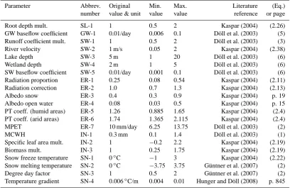
Table 1. Detailed information on the calibration parameter (col. 1; MCWH: maximum canopy water height, MPET: maximum potential
evapotranspiration, PT: Priestley-Taylor) is provided by belonging processes and numbering (col. 2; SL: Soil, GW: groundwater, SW: Surface water, ER: Evaporation and Radiation, SN: Snow, IN: Interception), original WGHM value (col. 3), minimum and maximum value (col. 4, 5). Literature references for the model parameter and according equation numbers are provided in columns 6 and 7.
Parameter Abbrev. Original Min. Max. Literature (Eq.) number value & unit value value reference or page Root depth mult. SL-1 1 0.5 2 Kaspar (2004) (2.26) GW baseflow coefficient GW-1 0.01/day 0.006 0.1 D¨oll et al. (2003) (5) Runoff coefficient mult. SW-1 1 0.5 2 D¨oll et al. (2003) (3) River velocity SW-2 1 m/s 0.05 2 Kaspar (2004) (2.38) Lake depth SW-3 5 m 1 20 D¨oll et al. (2003) (6) Wetland depth SW-4 2 m 1 5 D¨oll et al. (2003) (6) SW baseflow coefficient SW-5 0.01/day 0.001 0.1 D¨oll et al. (2003) (6) Radiation proportion ER-1 0.25 0.08 0.54 Kaspar (2004) (2.11) Radiation correction ER-2 1.0 0.7 1.3 Kaspar (2004) (2.13) Albedo snow ER-3 0.4 0.3 0.9 Kaspar (2004) p. 19 Albedo open water ER-4 0.08 0.03 0.5 Kaspar (2004) p. 15 PT coeff. (humid areas) ER-5 1.26 0.885 1.65 Kaspar (2004) (2.4) PT coeff. (arid areas) ER-6 1.74 1.365 2.115 Kaspar (2004) (2.4) MPET ER-7 10 mm/day 6.25 13.75 D¨oll et al. (2003) (2) MCWH IN-1 0.3 mm 0.1 1.4 D¨oll et al. (2003) (1) Specific leaf area mult. IN-2 1 −0.2 2.2 Kaspar (2004) (2.19) Biomass mult. IN-3 1 0.25 1.75 Kaspar (2004) (2.19) Snow freeze temperature SN-1 0◦C −1 3 Kaspar (2004) (2.22) Snow melting temperature SN-2 0◦C −3.75 3.75 G¨untner et al. (2007) (2) Degree day factor SN-3 1 0.5 2 G¨untner et al. (2007) (2) Temperature gradient SN-4 0.006◦C/m 0.004 0.01 Hunger and D¨oll (2008) p. 845
water albedo (ER-4) and sublimation of snow by the snow albedo (ER-3). Land surface evapotranspiration is limited by the maximum potential evapotranspiration (MPET, ER-7) parameter (see D¨oll et al., 2003).
Interception storage capacity depends on three parame-ters: The maximum canopy water height (MCWH, IN-1), a specific leaf area multiplier (IN-2), and a biomass multiplier (IN-3).
The rates of snow melting and accumulation depend on land cover and elevation. Snow melting is computed in WGHM by a degree-day approach. The degree-day factor depends on the type of land cover and is calibrated in this study by a multiplicative factor (SN-3). Sub-grid variability of elevation within a 0.5-degree model cell is represented in WGHM (100 sub-units per 0.5◦-cell) and elevation effects are accounted for by a temperature gradient (SN-4). Addi-tional effects on snow storage processes can be adjusted by a cell-averaged snow freeze temperature (SN-1) and snow melting temperature (SN-2).
2.2 Calibration technique
2.2.1 Calibration regions and parameter sensitivity
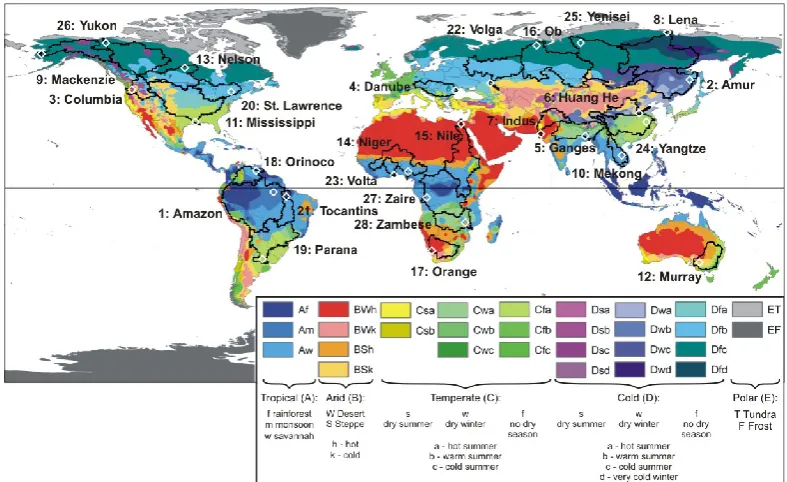
Due to the limited resolution of GRACE data, the 28 largest and most important river basins worldwide were selected for this study (Fig. 1). With the exception of Volta in western Africa, all basins are larger than 600 000 km2 in size (see Table 2). WGHM calibration is carried out separately for each basin.
Fig. 1. The 28 largest and most important river basins worldwide (black polygons) with underlying K¨oppen-Geiger climate zones from
1951–2000 (Peel et al., 2007) and gauging stations (white diamonds) of each basin that was used for the calibration of river discharge. See Table 2 for station names.
discharge (Table 3) were used for the regional calibration of each river basin. Non-sensitive parameters were set to their original values (Table 1, col. 3).
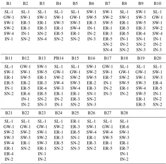
The results of the SA confirmed that the subset of sensitive parameters varied considerably across the river basins. While snow parameters are not sensitive in tropical basins, param-eters that control surface water transport appeared to be par-ticularly sensitive in basins with important flood plains, such as the Amazon. A broader range of sensitive parameters was visible in the Indus river basin, which is dominated by snow storage in the northern mountain area and has high evapora-tion rates in the desert region of the lower Indus. Hence, sen-sitive parameters belong to these two processes and soil wa-ter paramewa-ters are comparatively less important in the Indus basin. The important parameters for the Mississippi cover a variety of processes (soil, snow, evaporation, interception, and surface water) because this river basin stretches across three different climate regions (cold in the north, subtropical in the southeast, and dry in the southwest).
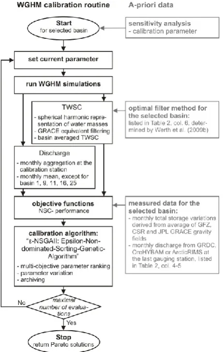
2.2.2 Multi-objective calibration approach
The Pareto-based multi-objective calibration approach that is used for WGHM was explained in detail by Werth et al. (2009a). Figure 2 and the description below provide an overview of this method. Calibration was performed for all 28 river basins in an automated framework for the period of time spanning January 2003–December 2007.
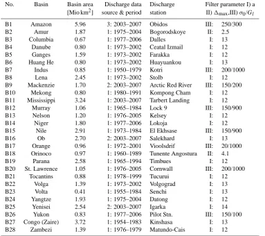
Table 2. Details of the 28 calibrated river basins (col. 1–3) and calibration data (col. 4–6) used. Col. 4: River runoff station, col. 5: Source
of discharge data (1: GRDC, 2: US-ACE, 3: ORE-HYBAM) and period runoff data applied for calibration, col. 6: applied GRACE filter method and belonging filter parameter (I: isotropic filter of Swenson and Wahr (2002) for an a-priori given maximum error of basin average
1max; II: Swenson and Wahr (2002) computed by the auto-correlation lengthGland standard deviationσ0of an exponential signal model;
III: decorrelation method by Kusche (2007) with the powerxfor the regularisation factora=10xof the signal covariance matrix).
No. Basin Basin area Discharge data Discharge Filter parameter I) a [Mio km2] source & period station II)1max,III)σ0/Gl
B1 Amazon 5.96 3: 2003–2007 Obidos III: 250/300 B2 Amur 1.87 1: 1975–2004 Bogorodskoye II: 2.5 B3 Columbia 0.67 1: 1977–2006 Dalles I: 13 B4 Danube 0.80 1: 1973–2002 Ceatal Izmail I: 12 B5 Ganges 1.59 1: 1973–2002 Farakka I: 12 B6 Huang He 0.80 1: 1973–2002 Huayuankou I: 13 B7 Indus 0.85 1: 1950–1979 Kotri III: 200/1000 B8 Lena 2.45 1: 1973–2002 Stolb I: 12 B9 Mackenzie 1.70 2: 2003–2007 Arctic Red River III: 150/200 B10 Mekong 0.80 1: 1980–1991 Kompong Cham I: 12 B11 Mississippi 3.24 1: 2003–2007 Tarbert Landing I: 12 B12 Murray 1.06 1: 1965–1984 Lock 9 III: 150/900 B13 Nelson 1.20 1: 1976–2005 Kelsey I: 12 B14 Niger 1.80 1: 1977–2006 Lokoja I: 12 B15 Nile 2.91 1: 1973–1984 El Ekhsase III: 150/900 B16 Ob 2.70 2: 2003–2007 Salekhard I: 13 B17 Orange 0.96 1: 1972–2001 Vioolsdrif III: 20/1000 B18 Orinoco 0.97 1: 1960–1989 Tunente Angostura II: 4.1 B19 Parana 2.58 1: 1965–1994 Timbues I: 12 B20 St. Lawrence 1.05 1: 1976–2005 Cornwall III: 200/1000 B21 Tocantins 0.88 1: 1978–1999 Tucurui I: 12 B22 Volga 1.39 1: 1973–2002 Volgograd I: 13 B23 Volta 0.41 1: 1955–1984 Senchi I: 13 B24 Yangtze 1.93 1: 1975–2004 Datong I: 12 B25 Yenisei 2.54 2: 2003–2007 Igarka I: 14 B26 Yukon 0.83 1: 1977–2006 Pilot Stn. III: 150/100 B27 Congo (Zaire) 3.72 1: 1954–1983 Kinshasa I: 13 B28 Zambezi 1.39 1: 1976–1979 Matundo-Cais I: 12
Without additional information on factors such as the reli-ability of the observation data or a pre-defined priority of calibration success for one of the objectives, all Pareto so-lutions are equally valid optimal model runs. In order to define the parameter set after calibration that produced the most balanced model improvement with regard to both ob-jectives (river discharge and TWSV), the Pareto solution that was closest to the optimum of the objectives (here a value of NSC=1 for both objectives) was selected in this study as the best parameter set and was used for further analyses.
The -Non-dominated Sorting Genetic Algorithm-II (-NSGAII, Kollat and Reed, 2006) was used to vary, rank, and archive the parameter sets during the WGHM pro-cess. The multi-start scheme and the evolutionary strat-egy of the algorithm (mutation, crossover, and selection) enable a global optimisation of the parameter values and are able to solve highly non-linear optimisation problems. This algorithm is one of the most efficient and effective
multi-objective optimisation methods used in hydrological modelling (Tang et al., 2006). These features enable a Pareto-based multi-objective calibration for more than one parame-ter of the non-linear and computationally expensive WGHM model system. -NSGAII operators were set to the values proposed by Kollat and Reed (2006), and a population size of N=12, an-resolution of 0.05 for both objectives, and a generation size of 100 (a maximum of 1200 model evalua-tions) were used.
Fig. 2. The concept scheme of multi-objective WGHM calibration
for a specific river basin using input from Werth et al. (2009b) for applied GRACE filter methods.
2.3 Calibration data
2.3.1 Discharge data
River discharge data for the most downstream gauging sta-tion of each river basin were used (Table 2, col. 4 and Fig. 1). Data were obtained from the Arctic Regional Integrated Hydrological Monitoring System for the Pan-Arctic Land Mass (Pan-ArcticRIMS, http://rims.unh.edu), the Environmental Research Observatory for geodynamical, hy-drological and biogeochemical control of erosion/alteration and material transport in the Amazon (ORE HYBAM, http://www.ore-hybam.org/), and the Global Runoff Data Center (GRDC, http://www.bafg.de/GRDC/EN/).
Monthly discharge data were available for the GRACE operation period for the Amazon, Mississippi, Mackenzie, Ob and Yenisei basins. For all other basins, up-to-date measurements were not available and mean monthly river discharge (for January–December) was computed from the
most recent period of available data (maximum period of 30 years, see Table 2).
Errors in discharge measurements depend on the individ-ual measurement methods and channel cross-sections are likely to vary for the individual stations and time periods. Unfortunately, the data centres do not provide details on the accuracy of discharge measurements. Therefore, the error in discharge measurements was set to a conservative value of 20% for the uncertainty analysis of the calibration results.
2.3.2 GRACE data
GRACE data used in this study were provided in the form of a monthly spherical harmonic representation of the gravity field (Level-2 products, most recent release RL04) by three different processing centres: the German Research Center for Geosciences (GFZ, until spherical harmonic degree 120), the Center for Space Research (CSR, until degree 60), and the Jet Propulsion Laboratory (JPL until degree 120). Atmo-spheric and oceanic gravity effects have been removed from the GRACE gravity fields by all centres (Flechtner, 2009). The three data sets show significant differences (see, e.g. the Lena basin in Fig. 3), which are due to different process-ing strategies, background models, or processprocess-ing software (Schmidt et al., 2008a). An average of GRACE gravity fields from three processing centres was used for the present study and the differences between the data sets were considered as a measure of uncertainty in GRACE TWSC data (see details below). The three sets of coefficients were averaged from degree 2 to 60 for each month in the period ranging from February 2003 to December 2008, excluding June 2003 and April 2004 due to missing data from GFZ. For GFZ, regu-larised solutions for July–October 2004 and December 2006 were applied.
The method to transform the spherical harmonic coeffi-cients of GRACE gravity fields to regional averaged water mass variations by Swenson and Wahr (2002) was applied using river basin boundaries (Fig. 1). Long-term trends deter-mined from both the hydrology model WGHM and from the GRACE gravity fields were removed from the TWSV time series in this study.
Table 3. Most sensitive calibrated parameter for the 28 river basins. See Tables 1 and 2 for complete basin names and parameter description.
B1 B2 B3 B4 B5 B6 B7 B8 B9 B10 SL-1 SL-1 SL-1 SL-1 SL-1 SW-1 SW-1 SL-1 SW-1 SL-1 GW-1 SW-1 SW-1 SW-1 GW-1 SW-5 SW-2 SW-1 SW-3 GW-1 SW-1 ER-3 ER-1 SW-3 SW-3 ER-3 SW-5 ER-1 SW-5 SW-1 SW-2 ER-1 ER-3 ER-1 SW-4 IN-1 ER-1 ER-3 ER-3 SW-2 SW-4 IN-1 SN-2 ER-5 ER-1 IN-2 ER-3 ER-5 ER-4 SW-4 IN-1 SN-2 SN-4 SN-2 SN-2 IN-3 ER-5 IN-1 SN-1 IN-1
SN-2 IN-2 SN-2 IN-2 SN-4 SN-2 SN-3 IN-3 B11 B12 B13 PB14 B15 B16 B17 B18 B19 B20 SL-1 GW-1 SW-1 SL-1 SL-1 SW-1 GW-1 SL-1 SL-1 SL-1 SW-1 SW-1 SW-5 GW-1 GW-1 SW-2 SW-1 GW-1 GW-1 SW-1 ER-1 SW-5 ER-1 SW-2 SW-2 SW-5 ER-7 SW-2 SW-1 SW-3 ER-5 ER-2 ER-3 SW-4 SW-3 ER-2 IN-1 SW-5 SW-3 ER-4 IN-1 ER-5 ER-4 SW-3 SW-4 ER-3 IN-2 ER-1 SW-4 ER-5 SN-2 ER-6 ER-5 ER-1 ER-1 SN-1 IN-3 IN-2 SW-5 IN-1 IN-1 SN-2 IN-2 ER-3 SN-2 ER-1 IN-2 IN-2 SN-3 IN-1 SN-2 SN-3 ER-5 SN-2 B21 B22 B23 B24 B25 B26 B27 B28
SL-1 SL-1 SL-1 SL-1 ER-1 SL-1 SL-1 SL-1 GW-1 GW-1 GW-1 SW-2 ER-3 SW-1 GW-1 ER-6 SW-2 SW-2 SW-1 ER-1 ER-5 SW-4 SW-4 SW-1 SW-3 SW-3 SW-2 ER-3 SN-1 ER-1 SW-5 SW-3 SW-4 ER-1 SW-3 ER-5 SN-2 ER-3 ER-1 ER-1 ER-1 SN-2 ER-1 SN-2 SN-3 SN-2 ER-5 ER-7
ER-4 IN-1 IN-1
[image:8.595.71.524.454.651.2]IN-2 IN-2 IN-2
Fig. 3. Basin-averaged time series of TWS variations from GRACE for the Lena river basin from the processing centres CSR (green), GFZ
data. Consequently, the error budget of derived TWSV is also influenced by signal leakage errors from surrounding areas.
The selection of an optimal filter method that leads to a proper error reduction as well as to a sufficient separa-tion of signal from the region of interest and its neighbour-ing regions is one of the greatest challenges when resolv-ing GRACE data for TWSV. Filterresolv-ing might change the fi-nal TWSV sigfi-nal properties and the magnitude of errors varies between particular regions and months. Werth et al. (2009b) showed that filter-induced amplitude damping and phase shifts in the time series of basin-averaged TWSV dif-fers between regions due to varying signal characteristics in-side and outin-side of the river basin as well as the basin shape. Therefore, the user must decide on an adequate filter method and adequate filter parameters for each river basin specifi-cally in order to optimally balance and minimise GRACE measurement errors and leakage errors.
In the present study, the optimal filter methods and fil-ter paramefil-ter values of Werth et al. (2009b) were applied to smooth GRACE and hydrological data from 22 river basins. Optimal filter settings were derived by repeating the method that is described by Werth et al. (2009b) for the remaining six basins (Columbia, Huang He, Mekong, Murray, Orinoco and Volta). See Table 2 for a summary of applied filter meth-ods. The optimal spatial resolution varies between 200 and 600 km (see Werth et al. (2009b), Table 5, col. I with the val-ues for each river basin), though resolutions achieved in the present study are likely to be higher since filtering methods that are more sophisticated than the Gaussian were used for each basin.
All processing centres publish GRACE errors as errors of the spherical harmonic coefficients. Since errors are too op-timistic if they are derived from the adjustment equation sys-tem that is used to process GRACE gravity fields, the GFZ and CSR processing centres adjust them to apparent signal noise in the spatial domain (Schmidt et al., 2008a; Wahr et al., 2006). Such correlated errors were not available for JPL gravity fields. Therefore, assuming a normal distribution of the GRACE errors, the confidence interval of the JPL coef-ficient error assessment was increased to 99% for this study. This results in a≈2.6-times greater error than the original JPL coefficient errors. According to the law of error propa-gation, the final error for the averaged coefficients from the three processing centres amounts to:
knmavefield= q
knmGFZ2+knmCSR2+knmJPL2, (1)
k= [0,1], n= [2,60], m= [0,60] .
[image:9.595.312.542.61.216.2]Subsequently, errors in the coefficients are propagated to basin averages of water storage for each river basin. Fig-ure 3 provides an example of basin-averaged TWSV that is derived from the three gravity solutions, the average solution, and associated errors.
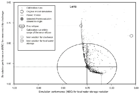
Fig. 4. Calibration results for the Lena river basin in terms of
ob-jective function values. Each point (gray and black) represents one model run. The Pareto optimal solutions form a frontier (gray solid line) toward the optimal model fit (lower left corner). The Pareto so-lution closest to the optimum (gray large dot) is selected as the op-timal solution of the calibration providing a balanced improvement for both objectives and is used for further studies. Best solutions for the single objectives are located at the end of the Pareto fron-tier (crossed large dots). An uncertainty range for both objectives is indicated by an error ellipse around the selected Pareto solution from errors of the measured calibration data. The solutions lying in that range (black small dots) show a significant improvement in the calibrated model compared to the original model simulation (plain black circle).
2.4 Uncertainty estimation due to observational errors
The uncertainty of the calibration results due to errors in the calibration data is estimated for each river basin by the fol-lowing procedure: 1) Selection of the calibration run with the Pareto solution closest to the optimum (see an example for the Lena river basin in Fig. 4). 2) Propagation of GRACE co-efficient errors to basin-averaged estimates of TWSV as well as determination of the 20% discharge error. 3) Generation of 5000 normally-distributed samples within the estimated error ranges for the monthly data points of GRACE-based TWSV and monthly river discharge, respectively. The sam-ple size was tested ahead of time and selected to provide sta-ble statistical results. 4) Estimation of the objective functions (NSC) for each sample against simulated time series of the selected optimal solution for TWSV and discharge, respec-tively. 5) Determination of the NSC standard deviations for both objectives as the semi-axis for an error ellipse around the selected optimal solution. And 6) Selection of all cali-bration runs within the error ellipse (see Fig. 4 for the Lena basin).
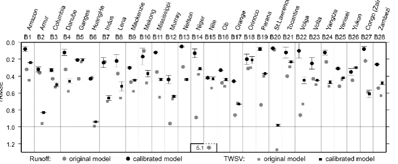
Fig. 5. Simulation performance for the 28 calibrated river basins in terms of relative root mean squared error (rRMSE) for river discharge
(circles) and TWSV (squares) of the original (gray) and the calibrated model version (black) (see Table 4 for absolute values). Error bars are derived from GRACE and discharge measurement errors as described in Sect. 2.4.
3 Results and discussion
3.1 Calibration results
Detailed results for Lena basin (Fig. 4) demonstrate a typi-cal objective function response that was found following the calibration of most river basins. A clear trade-off exists be-tween both objective functions for TWSV and mean monthly discharge. The best solutions for the single objectives are lo-cated at the end of the Pareto frontier (crossed dots). Best results for a single objective, however, give an undesirable decrease in the accuracy for the other objective. The selected Pareto optimum (large gray dot) provides a balanced im-provement between both objectives. The multi-objective cal-ibration approach also decreases equifinality of the parameter sets since unacceptable parameter sets for any of the objec-tives are excluded by the multi-objective evaluation scheme. A more pronounced equifinality for simulating total water storage variations originates from the nature of total water storage data. GRACE provides no absolute values but only variations in water masses. Therefore, the same storage vari-ations may be simulated by different model representvari-ations with different absolute amounts of water stored in the river basin. This is not the case for river discharge where both absolute values and variations are given by the observation data. Hence, a smaller number of model realisations pro-vide good objective values for evaluation by discharge than by TWSV. The large ellipse around the selected Pareto op-timum represents its uncertainty caused by measurement er-rors in the calibration data. Variations in parameter values or model output for model realisations within this range are not significant for the assumed observation data errors. Nev-ertheless, a significant improvement was achieved for both objective values relative to the original model in the analysis of the Lena basin.
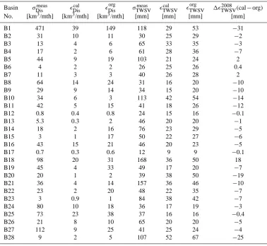
Table 4. Root mean squared signal of observed river discharge (σDismeas, col. 2) and standard deviation of GRACE TWSV (σTWSVmeas , col. 5) compared to the root mean squared error (RMSE) of the calibrated (cal, col. 3 and 6) and the original (org, col. 4 and 7) model against respective observation data for all 28 river basins. Column 8 provides differences of RMSE values of TWSV from the calibrated and the original model for the validation period (January 2008–December 2008). Here, negative values indicate an improved simulation of the calibrated compared to the original model.
Basin σDismeas Discal Disorg σTWSVmeas TWSVcal orgTWSV 1TWSV2008 (cal−org)
No. [km3/mth] [km3/mth] [km3/mth] [mm] [mm] [mm] [mm] B1 471 39 149 118 29 53 −31
B2 31 10 11 30 25 29 −2
B3 13 4 6 65 33 35 −3
B4 17 2 6 61 28 36 −7
B5 44 9 19 103 21 24 2
B6 4 2 2 26 25 26 0.4
B7 11 3 3 40 26 28 2
B8 64 14 24 31 16 20 −10
B9 29 9 14 34 15 20 −10
B10 34 6 3 113 42 54 −14
B11 42 5 15 41 18 26 −12
B12 0.8 0.4 0.8 24 15 16 −0.1
B13 5.3 0.3 2 46 20 20 −1
B14 18 2 16 76 23 29 −5
B15 3 1 17 50 22 27 −6
B16 43 15 21 46 20 23 −5
B17 0.7 0.3 0.6 12 9 9 −0.1
B18 98 20 31 168 36 50 18
B19 45 4 33 49 17 20 −7
B20 20 1 2 39 38 50 −19
B21 36 4 14 157 36 46 −10
B22 23 2 20 48 22 35 −7
B23 3 0.9 1 84 38 42 −7
B24 80 10 18 36 17 19 −3
B25 73 23 38 37 16 16 −0.4
B26 21 8 10 65 20 20 −5
B27 112 9 25 41 25 24 −4
B28 9 2 5 107 52 67 −25
With the selected optimum parameter sets, WGHM simulations were repeated between January 2008– December 2008 beyond the calibration period for validation against the GRACE-based TWSV. Table 4 shows that the improvement relative to the original model is similar to the calibration period for most of the river basins. For example, RMSE differences from the original model are promising for the Amazon (31 mm≈26%), the Lena (10 mm≈32%), Mackenzie (10 mm≈29%), Mekong (14 mm≈12%), St. Lawrence (19 mm≈49%), and Zam-bezi (25 mm≈23%). Only a slight improvement in the TWSV simulation is achieved in the validation period for the Murray, Nelson, Orange and Yenisei. A larger RMSE than for the original model was found for the Ganges, Huang He, Indus, Orinoco, Nelson, Orange, and Congo. This corresponds to the calibration failure of the latter three basins mentioned above.
3.2 Simulation of seasonal TWSV
Fig. 6. Results for seasonal amplitude (circles) and phase (squares) of TWSV for the original (gray) and the calibrated model version (black)
compared to GRACE (red). Error bars for TWSV amplitudes are derived from GRACE and discharge measurement errors as described in Sect. 2.4.
3.3 Parameter values and single storage compartments
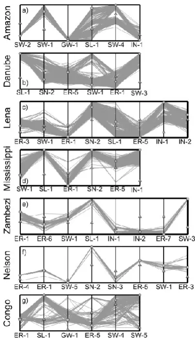
A detailed analysis of parameter changes (Fig. 7) and their effects on single storage compartments (Fig. 8–11) is pro-vided for seven river basins from different continents, cli-matic conditions, and with different calibration successes. Storage in lakes, floodplains, and wetlands (denoted surface water) is analysed separately from water in the river channel (denoted river storage) in the following sections.
AMAZON. The improved representation of TWSV simula-tions for the tropical Amazon after multi-criterial calibration is mainly due to a lower river flow velocity (SW-2) in the cal-ibrated model version and a larger runoff coefficient (SW-1). The adjustment of both parameters is stable against calibra-tion uncertainty from observacalibra-tion errors (Fig. 7a). The pa-rameter changes cause a longer-lasting storage of more water in the river network that leads to larger and delayed seasonal amplitudes of TWS, which is in line with GRACE observa-tions (Fig. 8a). Furthermore, inter-annual variaobserva-tions of TWS, such as the heavy drought that was experienced in the Ama-zon in 2005 (Zeng et al., 2008), are better represented with the calibrated model (Fig. 8a). A slightly increased soil wa-ter storage is due to the larger rooting depth (SL-1) in the re-calibrated model. However, the rooting depth parameter is
highly uncertain and it is not significant relative to the orig-inal model. This can be seen in the wide spread of param-eter values for the Pareto solutions in Fig. 7a. The larger value for the parameter wetland depth (SW-4) has nearly no effect on the storage variability in lakes and wetlands de-spite the great importance of wetlands and floodplains for water storage in the Amazon (Papa et al., 2008). Surface water storage is mainly attributed to river channel storage in WGHM (Fig. 8a), although the large inundation areas are taken into account as model input. This might indicate struc-tural model errors in representing surface water exchange processes between floodplains and the channel due to the conceptual model formulations and the cell-based simulation of surface water bodies in WGHM.
and soil storage are supported by a lower radiation propor-tion absorbed by the surface, which leads to higher snow ac-cumulation as well as a delayed snow melting. Compared to the original model, these parameter changes for the Mis-sissippi are reliable considering the calibration uncertainty (Fig. 7d). An earlier seasonal peak of simulated TWS com-pared to GRACE data (see Fig. 8b) might be attributed to underestimated groundwater storage that is typically charac-terised by a later seasonal phase compared to near-surface storage. In fact, studies by Rodell et al. (2007) and Zaitchik et al. (2008) demonstrate a higher groundwater volume than was represented by WGHM. A change for groundwater was prevented by the missing sensitivity of the groundwater pa-rameter for WGHM (B11 in Table 3), which might be due to the overlap with soil storage variations. The groundwater parameters should therefore be included in further calibration studies.
LENA. In the Lena basin, the seasonality of river water storage exhibits an opposite phase to total storage, which is dominated by snow storage variations. This makes a fit of the overall small TWSV amplitude (below 50 mm w.eq. on aver-age) more difficult than for the two previous basins. Model improvements by calibration for this cold, high-latitude basin (Fig. 1) are mainly temporal. The phase of TWSV could be corrected (Fig. 6) based on changes in water accumulation in snow, the river, and soil (Fig. 9a). Due to a higher snow melting temperature (SN-2), snow accumulation lasts nearly one month longer and snow melting finally occurs later but more rapidly during April and May. The larger snow albedo (ER-3) decreases snow sublimation and supports the slightly larger variability in snow storage. In line with later and faster snow melting in the spring, water storage dynamics in the river network change accordingly. A larger and later monthly runoff peak also corresponds to the river discharge measure-ments and is better represented by the calibrated model (see embedded graph in Fig. 9a). Changes in the soil storage dy-namics due to calibration are of minor importance in the Lena basin. In general, they are characterised by slightly larger seasonal variations with a later phase commensurate to the snow dynamics but also to overall lower evapotranspiration rates caused by smaller radiation proportion (ER-1) and PT-coefficient (ER-5) parameters.
[image:13.595.325.527.60.411.2]DANUBE. Similar to Lena, mainly a phase correction of TWSV was achieved by calibration (Fig. 6) for the cold and partly temperate (Fig. 1) Danube basin. This resulted in a smaller RMSE of TWSV time series (Fig. 5). While the seasonal amplitude was not changed, a better fit for ex-treme events such as heat waves or floods (Andersen et al., 2005; Seitz et al., 2008) is visible in the time series for the autumns of 2003, 2005, and 2006, as well as for the water mass maxima in 2004 and 2006 (Fig. 9b). In the calibrated model, snow is melting faster due to a higher snow melt-ing temperature, hence reducmelt-ing the snow storage volume. The released water is mainly stored in the soil that has an in-creased storage capacity due to a larger root depth parameter
Fig. 7. Normalised parameters for exemplary river basins (a–g).
Parameter sets are shown for the selected optimum (circular sym-bols), the original model version (triangles), and all calibration runs within the uncertainty range (gray solid lines) due to observational errors.
after calibration. Additionally, river water is reallocated to the soil where it can remain for longer periods than in the quickly draining river network during the spring season. The smaller river discharge in spring is confirmed by observations (not shown here, due to limited space) resulting in a smaller RMSE for the mean monthly discharge (Fig. 5). Groundwa-ter storage variations slightly decreased and were delayed in the Danube basin.
Fig. 8. Basin-averaged time series of single storage compartments from the calibrated and the original model version (unsmoothed, below) as
well as smoothed total storage from both model versions and GRACE (smoothed, above) for (a) the Amazon and (b) the Mississippi basins. See Fig. 11 for the legend.
[image:14.595.122.473.399.689.2]Fig. 10. Same as Fig. 8 but for (a) the Zambezi and (b) the Nelson basins.
observation of increased groundwater volume, which con-firms the high relevance of water exchange with deeper soil zones for the Zambezi basin (Winsemius et al., 2006a). Sur-face water volume changes in wetlands increase after calibra-tion and result in longer residence times of water in the Zam-bezi basin. The importance of this storage mechanism in the Zambezi basin was also noted by Winsemius et al. (2006a).
NELSON. The seasonality of snow and groundwater stor-age exhibits a marked anti-phase in the Nelson basin ac-cording to the WGHM simulation results (Fig. 10b). This decreases model sensitivity for TWS variations and makes an effective calibration of the individual storage components difficult, since many combinations of different snow and groundwater states can lead to an equally good fit of sim-ulated to GRACE-based TWSV. In addition, the required smoothing of GRACE data has a huge effect on overall water storage dynamics for this basin (Fig. 10b). Major seasonal signals are smoothed, but the remaining TWSV time series correspond reasonably well between GRACE and WGHM. Comparatively small changes occur by model re-calibration relative to the original model.
CONGO. TWSV in the Congo (Zaire) basin is domi-nated by inter-annual patterns such as the water loss that occurred between 2003 and 2005 (Crowley et al., 2006). As assumed by Crowley et al. (2006), the loss is not sec-ular and the storage is filled up again during 2006 and 2007 (Fig. 11). Although the calibrated WGHM exhibits an
improved simulation for the seasonal amplitude and phase of the Congo basin (Fig. 6), the simulated inter-annual vari-ability of basin-average TWS is still different from GRACE, e.g. a too large negative anomaly in 2005. Also, RMSE values did not improve after calibration (Table 4). The inter-annual variations in TWS mainly derive from soil and groundwater storage (Fig. 11). For the calibrated model, a larger seasonal variability in soil storage causes a slightly de-layed phase of storage variability. This delay appears to be compensated by a negative phase shift in groundwater. As a result, the faster outflow of the groundwater due to a larger outflow coefficient GW-1 causes a smaller groundwater vol-ume and decreases the inter-annual variation of groundwater storage in the calibrated model.
Fig. 11. Same as Fig. 8 but for the Congo basin.
additional drawback for the Congo is that the available dis-charge data for this basin are only from 1954–1983.
The water mass variations of the Orange basin, which also exhibit inter-annual variations (not shown), are smaller than 12 mm of a water column (see Table 4, Fig. 6) and are below GRACE data accuracy for some months. While inter-annual variations are not relevant for the Yukon basin, a clear anti-phase between snow and groundwater storage as well as soil storage causes a small model sensitivity for TWS variations, similar to Nelson.
3.4 Global analysis
A global analysis of simulated TWSV for the calibrated model (see spatial distribution in Fig. 12 and variability of basin averages in Table 5) shows that its variability increased for most river basins compared to the original model. On the global average (last row of Table 5), TWS variabil-ity increased by 7 mm w.eq., which is mainly due to larger variations in soil, river, and surface water storage. Most variability is gained within the tropical and temperate re-gions, such as the Amazon (total 60 mm for the basin aver-age), Congo (9 mm), Niger (14 mm), Mekong (35 mm), and the Mississippi (14 mm). A spatial redistribution between sub-regions for some of these basins is visible in Fig. 12, e.g. Ganges and Parana. A smaller total water budget appears only for the basins in cold regions including the Mackenzie, St. Lawrence, Volga, and Yangtze (Table 5). Some further cold regions such as the Lena or Ob exhibit an unchanged water budget. This comparison shows that TWS variability in the original WGHM was mainly underestimated in tropi-cal and temperate regions but overestimated in cold regions, similar to the seasonal components (Fig. 6).
For the individual basins and storages, largest differences from the original model occur within soil storage, mainly for tropical and temperate regions such as the Mekong,
Mississippi, Orinoco, Volta, or Zambezi basins. This is vis-ible by area distributed TWSV differences compared to the original model (the lower section of Fig. 12) and is reflected in the basin averages (Table 5). Soil has the highest sea-sonal capacity to store water and contributes the most to the gravity signal discovered by GRACE, which is usually dom-inated by seasonal features. Linear structures in the spatial distribution of TWSV differences compared to the original model are mainly due to changes in river storage, the sec-ond greatest contributor to changes for the basin averages (Table 5). Very large increases in river water volumes occur in the rainy tropical regions of Amazon the, Mekong, and Orinoco, where a slow discharge in the river network causes a longer maintenance of river water in the basin (see analysis for Amazon in Sect. 3.3 above). In contrast, a decrease in river water volume is found in temperate and dry regions. Snow storage increases for regions in cold climate zones, such as the Columbia, Ob, and Yenisei basins. Snow stor-age decreases in cold climates that have warm summers, such as the St. Lawrence, Volga, and Danube. In these transition zones, less snow precipitation might be due to global climate warming, which is relevant for the calibration period but was not incorporated in the calibration of the original model.
Table 5. Variability of unfiltered and basin-averaged continental TWSV simulations from the calibrated WGHM version for total storage
and single compartments:σcal(storage)(TS: total storage, SL: soil, GW: groundwater, SN: snow, R: river, SW: surface water, C: canopy). Every other line provides deviations of storage variability to the original model:1σstorage=σcal(storage)−σorg(storage).
Basin σcal(TS) 1σTS σcal(SL) 1σSL σcal(GW) 1σGW σcal(SN) 1σSN σcal(R) 1σR σcal(SW) 1σSW σcal(C) 1σC
B1 150 +60 37 +8 25.7 +0.4 0.1 +0.0 82.9 +49.6 2.1 +0.8 0.0 +0.0
B2 20 +3 10 +3 7.8 −0.4 21.0 +1.7 5.0 +0.2 1.4 +0.2 0.5 +0.3
B3 55 −1 12 −7 4.4 −0.6 40.2 +6.1 3.5 +0.1 1.7 −0.2 0.2 +0.0
B4 64 +4 43 13 10.6 −2.2 16.0 −9.4 4.1 −3.0 1.4 +0.9 0.4 +0.0
B5 90 +7 17 −8 21.0 −5.6 1.8 +0.3 20.1 +3.6 10.6 +4.2 0.1 +0.1
B6 18 −2 9 +1 5.9 −1.4 0.3 +0.0 2.7 −0.6 0.3 −0.2 0.1 +0.1
B7 28 +4 7 +1 4.8 +0.7 24.6 +3.4 6.4 +0.2 1.0 +0.4 0.0 +0.0
B8 32 +0 8 +2 1.7 +0.2 47.9 +2.8 15.2 +4.7 1.8 +0.1 0.8 +0.5
B9 44 −8 7 −1 7.8 +0.5 50.7 +0.1 6.9 +3.5 1.5 −1.3 0.3 +0.0
B10 129 +36 54 +22 33.5 +0.6 0.3 +0.0 37.1 +11.2 3.1 +0.7 0.1 +0.1
B11 48 +14 27 +11 6.3 −0.4 12.1 +2.6 3.4 −0.6 1.9 +0.0 1.1 +0.9
B12 17 +3 9 +1 2.1 −0.6 0.0 +0.0 0.6 +0.4 2.4 +0.7 0.0 −0.1
B13 57 +2 10 −1 12.2 +1.2 39.8 +2.4 0.5 −0.2 7.7 +0.5 0.2 +0.0
B14 58 +14 26 +12 14.8 −4.6 0.0 +0.0 11.1 +4.2 3.2 −0.2 2.6 +2.6
B15 35 +2 21 +8 1.6 −5.3 0.0 +0.0 9.7 +1.2 3.5 +0.3 0.0 +0.0
B16 61 +0 14 −2 14.6 +2.2 67.5 +9.3 5.3 +0.4 1.5 −0.7 0.3 +0.0
B17 6 −1 3 −1 2.3 −0.3 0.0 +0.0 0.5 −0.3 0.4 −0.1 0.3 +0.3
B18 169 +51 57 +18 35.8 +1.7 0.0 +0.0 54.6 +26.0 7.6 +1.3 0.1 +0.0
B19 59 +1 22 +6 19.3 −0.8 0.0 +0.0 5.1 −10.3 5.6 +2.4 0.1 +0.0
B20 78 −20 15 −5 9.8 −4.9 43.4 −21.4 1.2 −1.4 9.2 −0.3 0.6 +0.3
B21 145 +18 39 +17 43.0 +0.8 0.0 +0.0 16.0 −9.4 13.1 +2.3 0.3 +0.3
B22 68 −16 33 +8 11.9 −2.6 56.0 −15.1 11.5 −5.4 1.7 +0.6 0.3 +0.0
B23 80 +26 49 +28 19.2 +1.9 0.0 +0.0 2.5 −0.4 4.6 −1.8 1.0 +1.0
B24 30 −5 4 −2 13.0 +1.2 1.2 +0.5 12.3 −3.4 0.7 +0.0 0.3 +0.0
B25 41 +2 9 +1 6.8 +1.3 56.0 +7.5 9.1 +3.9 1.9 +0.5 0.3 +0.0
B26 52 −3 7 +0 3.4 +0.3 57.6 +0.0 8.8 +1.1 2.9 +0.5 0.2 +0.0
B27 47 +9 26 +12 6.3 −8.8 0.0 +0.0 7.3 +1.2 2.8 +0.6 0.0 +0.0
B28 80 +26 41 +20 23.3 +5.3 0.0 +0.0 3.6 −0.7 9.1 +2.6 0.0 +0.0
global 66 +7 24 +3 15.4 −0.6 20.5 +0.2 9.4 +3.3 13.2 +2.7 0.2 +0.1
by the soil storage with a different seasonal phase. There-fore, future calibrations against GRACE data should include groundwater timing and volume parameters for each river basin.
Calibration results are also influenced by errors and un-certainties in climate data. Fiedler and D¨oll (2007) analysed those influences on WGHM model output and could show that uncertainties from climate input are smaller than differ-ences to GRACE for WGHM output.
4 Summary and conclusions
A consistent and globally-improved simulation of continen-tal water storage variations was achieved in this study by taking into account the following key points in a multi-objective calibration framework with GRACE water storage data: 1) Consistency of GRACE and model TWSV data by representing the most important storage compartments in the WGHM model (soil, snow, canopy, surface water, and groundwater). 2) Multi-objective calibration by absolute val-ues of river discharge and relative valval-ues of TWS variations. 3) Basin-specific calibration of the dominant processes by varying the most sensitive model parameters. 4) Consistency of the observables and model state variables (equal spatial
scale) by identical smoothing of GRACE and model data, as well as the application of the optimal filter method for each river basin. 5) Consideration of measurement errors in an uncertainty analysis of the calibration results.
The multi-objective calibration of WGHM led to improved simulation results, particularly for seasonal amplitudes and phases of both TWS variations and river discharge for most of the 28 calibrated river basins. TWS variability was largely increased for tropical regions in the calibrated model. A bet-ter representation of TWS variability in the calibrated model was corroborated by reasonable changes in simulated water storage in single storage compartments for seven river basins from different continents and diverse climatic regions. Addi-tionally, possible model structural errors were uncovered by the calibration, such as wetland volumes that are too low in the Amazon and the Mississippi basin.
Fig. 12. Global distribution of total storage variability of the
cali-brated WGHM (above) and its deviations to the original model ver-sion (below). Negative values below indicate decreased and positive values increased variability. Units are in mm of water column.
This will restrict the independence of observation data and model re-calibrations but also emphasises that the ment of large-scale hydrological models and the improve-ment of GRACE water mass estimates must be considered as an iterative process.
For some basins, errors or limitations in the calibration data restrict calibration success. The integrative nature of GRACE TWS data, their limited spatial resolution, and the lack of absolute water storage values imply that calibrating a hydrological model with GRACE data leaves the calibration results with a considerable degree of parameter equifinality. Considering the complex interaction between single storage components and the inability to separate these storages with the integrative TWSV data, GRACE data alone are not ade-quate to calibrate water storage state variables in large-scale hydrological models. Progress in remote sensing techniques for individual storages such as snow storage (e.g. by MODIS, Parajka and Bl¨oschl, 2008), surface water (Papa et al., 2008), or soil moisture from the upcoming satellite missions SMOS and SMAP are applicable for tuning or validating large scale-hydrological models with more than one or two objectives. An update of global river discharge data sets to the GRACE mission period is another urgent need for further progress.
Due to the large diversity of processes in different regions of manifold climatic conditions, global hydrological mod-elling is a challenging task. The present study expands ex-periences in the representation of hydrological processes to a global scale with a particular emphasis on water storage dynamics. The continuation of similar studies is further mo-tivated by the steadily improved accuracy of GRACE solu-tions and the future prospect of a GRACE follow-on mis-sion. Longer time series of gravity data will in particular allow focusing on hydrological extremes, inter-annual varia-tions, and secular trends in both observations and modelling capabilities.
Acknowledgements. We acknowledge J. Alcamo and P. D¨oll for
providing the WGHM model code. The German Ministry of Education and Research (BMBF) supported these investigations within the geoscientific R+D programme GEOTECHNOLOGIEN, “Erfassung des Systems Erde aus dem Weltraum”. The authors also want to thank Ross Woods for productive discussions about the calibration analysis methods.
Edited by: J. Liu
References
Alcamo, J., D¨oll, P., Henrichs, T., Kaspar, F., Lehner, B., R¨osch, T., and Siebert, S.: Development and testing of the WaterGAP 2 global model of water use and availability, Hydrolog. Sci. J., 48, 317–338, 2003.
Andersen, O. B., Seneviratne, S. I., Hinderer, J., and Viterbo, P.: GRACE-derived terrestrial water storage depletion associated with the 2003 European heat wave, Geophys. Res. Lett., 32, L18405, doi:10.1029/2005GL023574, 2005.
Beven, K. and Binley, A.: The future of distributed models: Model calibration and uncertainty prediction, Hydrol. Process., 6, 279– 298, 1992.
Crowley, J. W., Mitrovica, J. X., Richard, C. B., Tamisiea, M. E., and Davis, J. L.: Land water storage within the Congo Basin inferred from GRACE satellite gravity data, Geophys. Res. Lett., 33, L19402, doi:10.1029/2006GL027070, 2006.
Dirmeyer, P. A., Gao, X., Zhao, M., Guo, Z., Oki, T., and Hanasaki, N.: GSWP-2: Multimodel Analysis and Implications for Our Perception of the Land Surface, B. Am. Meteorol. Soc., 87, 1381–1397, 2006.
D¨oll, P. and Fiedler, K.: Global-scale modeling of groundwater recharge, Hydrol. Earth Syst. Sc., 12, 863–885, 2008.
D¨oll, P. and Lehner, B.: Validation of a new global 30-min drainage direction map, J. Hydrol., 258, 214–231, 2002.
D¨oll, P., Kaspar, F., and Lehner, B.: A global hydrological model for deriving water availability indicators: model tuning and vali-dation, J. Hydrol., 270, 105–134, 2003.
Fenicia, F., Savenije, H. H. G., Matgen, P., and Pfister, L.: Understanding catchment behavior through stepwise model concept improvement, Water Resour. Res., 44, W01402, doi:10.1029/2006WR005563, 2008.
Fiedler, K. and D¨oll, P.: Global modelling of continental water storage changes – sensitivity to different climate data sets, Adv. Goesci., 11, 63–68, 2007.
Flechtner, F.: GRACE Science Data System Monthly Report, Feb. 2009, Tech. rep., http://isdc.gfz-potsdam.de/, 2009.
Gulden, L. E., Rosero, E., Yang, Z.-L., Rodell, M., Jackson, C. S., Niu, G.-Y., Yeh, P. J. F., and Famiglietti, J.: Improving land-surface model hydrology: Is an explicit aquifer model better than a deeper soil profile?, Geophys. Res. Lett., 34, L09402, doi:10.1029/2007GL029804, 2007.
G¨untner, A.: Improvement of global hydrological models using GRACE data, Surv. Geophys., 29, 375–397, 2009.
G¨untner, A., Stuck, J., Werth, S., D¨oll, P., Verzano, K., and Merz, B.: A global analysis of temporal and spatial variations in continental water storage, Water Resour. Res., 43, W05416, doi:10.1029/2006WR005247, 2007.
Gupta, H. V., Sorooshian, S., and Yapo, P. O.: Toward improved calibration of hydrologic models: Multiple and noncommensu-rable measures of information, Water Resour. Res., 34, 751–763, 1998.
Gupta, H. V., Beven, K. J., and Wagener, T.: Model Calibration and Uncertainty Estimation, in: Encyclopedia of Hydrological Sciences, edited by: Anderson, M., Wiley, Chichester, 3, p. 131, 2005.
Han, S. C., Jekeli, C., and Shum, C. K.: Time-variable aliasing effects of ocean tides, atmosphere, and continental water mass on monthly mean GRACE gravity field, J. Geophys. Res., 109, B04403, doi:10.1029/2003JB002501, 2004.
Hornberger, G. M. and Spear, R. C.: An Approach to the Prelim-inary Analysis of Environmental Systems, J. Environ. Manage., 12, 7–18, 1981.
Horwath, M. and Dietrich, R.: Errors of regional mass variations inferred from GRACE monthly solutions, Geophys. Res. Lett., 33, L07502, doi:10.1029/2005GL025550, 2006.
Houtekamer, P. L. and Mitchell, H. L.: Data Assimilation Using an Ensemble Kalman Filter Technique, Mon. Weather Rev., 126, 796–811, 1998.
Hunger, M. and D¨oll, P.: Value of river discharge data for global-scale hydrological modeling, Hydrol. Earth Syst. Sci., 12, 841– 861, 2008,
http://www.hydrol-earth-syst-sci.net/12/841/2008/.
Kaspar, F.: Entwicklung und Unsicherheitsanalyse eines globalen hydrologischen Modells., Ph.D. thesis, Universit¨at Kassel, 2004. Kollat, J. B. and Reed, P. M.: Comparing state-of-the-art evolution-ary multi-objective algorithms for long-term groundwater moni-toring design, Adv. Water Resour., 29, 792–807, 2006.
Kollet, S. J. and Maxwell, R. M.: Capturing the influence of ground-water dynamics on land surface processes using an integrated, distributed watershed model, Water Resour. Res., 44, W02402, doi:10.1029/2007WR006004, 2008.
Kusche, J.: Approximate decorrelation and non-isotropic smooth-ing of time-variable GRACE-type gravity field models, J. Geodesy, 81, 733–749, 2007.
Legates, D. R. and Willmott, C. J.: Mean Seasonal and spatial vari-ability in gauge-corrected global precipitation, Int. J. Climatol., 10, 111–127, 1990.
Lettenmaier, D. P. and Famiglietti, J. S.: Hydrology: Water from on high, Nature, 444, 562–563, 2006.
Liu, J., Williams, J. R., Zehnder, A. J., and Yang, H.: GEPIC – modelling wheat yield and crop water productivity with high res-olution on a global scale, Agr. Syst., 94, 478–493, 2007. Liu, J., Zehnder, A. J. B., and Yang, H.: Global
consump-tive water use for crop production: The importance of green water and virtual water, Water Resour. Res., 45, W05428, doi:10.1029/2007WR006051, 2009.
Lo, M.-H., Yeh, P. J.-F., and Famiglietti, J.: Constraining water table depth simulations in a land surface model using estimated baseflow, Adv. Water Resour., 31, 1552–1564, 2008.
Lo, M.-H., Famiglietti, J. S., Yeh, P. J.-F., and Syed, T. H.: Improve parameter estimation and water table depth simulation in a land surface model using GRACE water storage and estimated base-flow data, Water Resour. Res., doi:10.1029/2009WR007855, in press, 2010.
Milly, P. C. and Shmakin, A. B.: Global modeling of land water and energy balances. Part I: The Land Dynamics (LaD) model, J. Hydrometeorol., 3, 283–299, 2002.
Nash, J. E. and Sutcliffe, J. V.: River flow forecasting through con-ceptual models part 1 – A discussion of principles, J. Hydrol., 10, 282–290, 1970.
Ngo-Duc, T., Laval, K., Ramillien, G., Polcher, J., and Cazenave, A.: Validation of the land water storage simulated by Organising Carbon and Hydrology in Dynamic Ecosystems (ORCHIDEE) with Gravity Recovery and Climate Experiment (GRACE) data, Water Resour. Res., 43, W04427, doi:10.1029/2006WR004941, 2007.
Niu, G.-Y., Yang, Z.-L., Dickinson, R. E., Gulden, L. E., and Su, H.: Development of a simple groundwater model for use in climate models and evaluation with Gravity Recovery and Climate Experiment data, J. Geophys. Res., 112, D07103, doi:10.1029/2006JD007522, 2007.
Papa, F., G¨untner, A., Frappart, F., Prigent, C., and Rossow, W. B.: Variations of surface water extent and water storage in large river basins: A comparison of different global data sources, Geophys. Res. Lett., 35, L11401, doi:10.1029/2008GL033857, 2008. Parajka, J. and Bl¨oschl, G.: The value of MODIS snow cover data in
validating and calibrating conceptual hydrologic models, J. Hy-drol., 358, 240–258, doi:10.1016/j.jhydrol.2008.06.006, 2008. Peel, M. C., Finlayson, B. L., and McMahon, T. A.: Updated world
map of the K¨oppen-Geiger climate classification, Hydrol. Earth Syst. Sci., 11, 1633–1644, 2007,
http://www.hydrol-earth-syst-sci.net/11/1633/2007/.
Priestley, C. H. and Taylor, R. J.: On the assessment of surface heat flux and evaporation using large-scale parameters, Mon. Weather Rev., 100, 81–92, 1972.
Reichle, R. H., McLaughlin, D. B., and Entekhabi, D.: Hydro-logic Data Assimilation with the Ensemble Kalman Filter, Mon. Weather Rev., 130, 103–114, 2002.
Rodell, M., Chen, J., Kato, H., Famiglietti, J., Nigro, J., and Wilson, C.: Estimating groundwater storage changes in the Mississippi River basin (USA) using GRACE, Hydrogeol. J., 15, 159–166, 2007.
Savenije, H. H. G.: HESS Opinions “The art of hydrology”*, Hy-drol. Earth Syst. Sci., 13, 157–161, 2009,
http://www.hydrol-earth-syst-sci.net/13/157/2009/.
Schmidt, R., Schwintzer, P., Flechtner, F., Reigber, C., G¨untner, A., D¨oll, P., Ramillien, G., Cazenave, A., Petrovic, S., Jochmann, H., and W¨unsch, J.: GRACE observations of changes in continental water storage, Global Planet. Change, 50, 112–126, 2006. Schmidt, R., Flechtner, F., Meyer, U., Neumayer, K. H., Dahle, C.,
K¨onig, R., and Kusche, J.: Hydrological signals observed by the GRACE satellites, Surv. Geophys., 29, 319–334, 2008a. Schmidt, R., Petrovic, S., G¨untner, A., Barthelmes, F., W¨unsch, J.,
and Kusche, J.: Periodic components of water storage changes from GRACE and global hydrology models, J. Geophys. Res., 113, B08419, doi:10.1029/2007JB005363, 2008b.
Schulze, K. and D¨oll, P.: Neue Ans¨atze zur Modellierung von Schneeakkumulation und -schmelze im globalen Wassermodell WaterGAP, in: 7th Workshop for large-scale modeling, in: Hy-drology. Munic, November 2003, edited by: Ludwig, R., Re-ichert, D., and Mauser, W., Kassel University Press, Kassel, 145– 154, 2004.
Seitz, F., Schmidt, M., and Shum, C. K.: Signals of extreme weather conditions in Central Europe in GRACE 4-D hydrological mass variations, Earth Planet. Sc. Lett., 268, 165–170, 2008.
Sheffield, J., Ferguson, C. R., Troy, T. J., Wood, E. F., and McCabe, M. F.: Closing the terrestrial water budget from satellite remote sensing, Geophys. Res. Lett., 36, L07403, doi:10.1029/2009GL037338, 2009.
Shuttleworth, W. J.: Evaporation, in: Handbook of hydrology, edited by: Maidment, D., McGraw-Hill Inc., 4.1–4.53, 1993. Swenson, S. and Wahr, J.: Methods for inferring regional
surface-mass anomalies from Gravity Recovery and Climate Experiment (GRACE) measurements of time-variable gravity, J. Geophys. Res., 107, 2193, doi:10.1029/2001JB000576, 2002.
Swenson, S., Famiglietti, J., Basara, J., and Wahr, J.: Estimating profile soil moisture and groundwater variations using GRACE and Oklahoma Mesonet soil moisture data, Water Resour. Res., 44, W01413, doi:10.1029/2007WR006057, 2008.
Syed, T. H., J. S., F., Rodell, M., Chen, J., and Wilson, C. R.: Analysis of terrestrial water storage changes from GRACE and GLDAS, Water Resour. Res., 44, W02433, doi:10.1029/2006WR005779, 2008.
Tang, Y., Reed, P., and Wagener, T.: How effective and efficient are multiobjective evolutionary algorithms at hydrologic model calibration?, Hydrol. Earth Syst. Sci., 10, 289–307, 2006, http://www.hydrol-earth-syst-sci.net/10/289/2006/.
Tapley, B. D., Bettadpur, S., Watkins, M., and Reigber, C.: The gravity recovery and climate experiment: Mission overview and early results, Geophys. Res. Lett., 31, L09607, doi:10.1029/2004GL019920, 2004.
Vrugt, J. A., Gupta, H. V., Bastidas, L. A., Bouten, W., and Sorooshian, S.: Effective and efficient algorithm for multiobjec-tive optimization of hydrologic models, Water Resour. Res., 39, 1214, doi:10.1029/2002WR001746, 2003.
Wahr, J., Swenson, S., Zlotnicki, V., and Velicogna, I.: Time-variable gravity from GRACE: First results, Geophys. Res. Lett., 31, L11501, doi:10.1029/2004GL019779, 2004.
Wahr, J., Swenson, S., and Velicogna, I.: Accuracy of GRACE mass estimates, Geophys. Res. Lett., 33, L06401, doi:10.1029/2005GL025305, 2006.
Werth, S., G¨untner, A., Petrovic, S., and Schmidt, R.: Integration of GRACE mass variations into a global hydrological model, Earth Planet. Sc. Lett., 277, 166–173, 2009a.
Werth, S., G¨untner, A., Schmidt, R., and Kusche, J.: Evaluation of GRACE filter tools from a hydrological perspective, Geophys. J. Int., 179, 1499–1515, doi: 10.1111/j.1365-46X.2009.04355.x, 2009b.
Widen-Nilsson, E., Halldin, S., and Xu, C.-y.: Global water-balance modelling with WASMOD-M: Parameter estimation and region-alisation, J. Hydrol., 340, 105–118, 2007.
Winsemius, H. C., Savenije, H. H. G., Gerrits, A. M. J., Zapreeva, E. A., and Klees, R.: Comparison of two model approaches in the Zambezi river basin with regard to model reliability and identifi-ability, Hydrol. Earth Syst. Sci., 10, 339–352, 2006a,
http://www.hydrol-earth-syst-sci.net/10/339/2006/.
Winsemius, H. C., Savenije, H. H. G., van de Giesen, N. C., van den Hurk, B. J. J. M., Zapreeva, E. A., and Klees, R.: Assessment of Gravity Recovery and Climate Experiment (GRACE) tempo-ral signature over the upper Zambezi, Water Resour. Res., 42, W12201, doi:10.1029/2006WR005192, 2006b.
Wouters, B., Chambers, D., and Schrama, E. J.: GRACE observes small-scale mass loss in Greenland, Geophys. Res. Lett., 35, L20501, doi:10.1029/2008GL034816, 2008.
Yapo, P. O., Gupta, H. V., and Sorooshian, S.: Mulit-objective global optimization for hydrologic models, J. Hydrol., 204, 83– 97, 1998.
Zaitchik, B. F., Rodell, M., and Reichle, R. H.: Assimilation of GRACE terrestrial water storage data into a land surface model: Results for the Mississippi River Basin, J. Hydrometeorol., 9, 535–548, 2008.