Seasonal Unit Root Tests: A Comparison

ZHANG, QIANYI. Seasonal Unit Root Tests: A Comparison. (Under the direction of Dr. David A. Dickey and Dr. Sastry G. Pantula .)

Three major regression-based seasonal unit root tests: the DHF test introduced by Dickey et al (1984), the HEGY test proposed by Hylleberg et al. (1990) and the Kunst test introduced by Kunst (1997) are compared. The regression model for the DHF test is a reduced form of that for the Kunst test. We modify the Kunst test by using the t-statistic instead of Kunst’s proposed joint F-statistic to study the influence of additional variables in the Kunst model. Also, we modify the HEGY test to test the presence of roots±1 and±iagainst the presence of roots±1. Through the comparison between the DHF test and the modified HEGY test, we find that the DHF test does not have an asymptotic power of one when the series only has some of the seasonal unit roots but not all of them. The asymptotic distributions derived in the paper provide the explanation of this limitation for the DHF test. Using simulation, we find that the probability that the DHF test fails to reject the seasonal unit root null hypothesis increases when the series contains more partial unit roots.

by

Qianyi Zhang

A dissertation submitted to the Graduate Faculty of North Carolina State University

in partial fulfillment of the requirements for the Degree of

Doctor of Philosophy

Statistics

Raleigh, North Carolina 2008

APPROVED BY:

Dr. David A. Dickey Dr. Sastry G. Pantula

Co-chair of Advisory Committee Co-chair of Advisory Committee

DEDICATION

BIOGRAPHY

ACKNOWLEDGMENTS

First of all, I owe a special word of thanks to my advisors Dr. David Dickey and Dr. Sastry Pantula for their guidance, time, and advice for my dissertation. They provided me with a tremendous amount of knowledge while still giving me the freedom to discover things on my own. I thank them for their encouragement to become an independent researcher. They are excellent statisticians and people. I am fortunate to work with them. I would also like to extend my sincere appreciation to my committee members for their contributions to the preparation of my dissertation. Thanks to Dr. Peter Bloomfield who provided helpful comments on the application to economic time series. Dr. Denis Pelletier also provided advice on getting the data for my analysis.

I am also thankful to Dr. Jacqueline Hughes-Oliver for her help and support during my program; I learned a lot of data mining techniques from her. I would like to thank Dr. Pam Arroway for her hard work to ensure the well-being of all students in the graduate program. I must thank Mr. Adrian Blue for his assistance in so many ways and Mr. Terry Byron for his professional technical support. My special thanks also go to Dr. Bibhuti Bhattacharyya, Dr. John Monahan, Dr. Leonard Stefanski, Dr. Sujit Ghosh and Dr. Hao Zhang for their wonderful lectures.

I would take the opportunity to thank my parents, who are always an unwavering source of support for me. They believe in me and encourage me in everything that I pursue. My parents have provided me with a tremendous amount of support. Without the love and support of my family, I would have never made it this far. Also, I am grateful for my friend, Yang Han, who encouraged me to keep trying when I thought I would never finish.

TABLE OF CONTENTS

LIST OF TABLES . . . vii

LIST OF FIGURES . . . ix

1 Introduction . . . 1

1.1 Statement of the Problem . . . 1

1.2 Literature Review . . . 3

1.2.1 Regression-Based Tests . . . 3

1.2.2 Graphical Test . . . 13

1.3 Summary of Chapters . . . 19

2 A Comparison of Seasonal Unit Root Test Criteria . . . 24

2.1 Motivations and Modifications . . . 24

2.2 Asymptotic Distributions . . . 27

2.2.1 Under the Null Hypotheses . . . 27

2.2.2 Under the Alternative Hypotheses . . . 41

2.3 Simulation Study . . . 56

2.3.1 Experimental Critical Values . . . 56

2.3.2 Empirical Powers . . . 59

2.4 Summary of Power Study . . . 84

3 Performance of Multiple-step Test Procedures . . . 87

3.1 Multiple-Step Test Criteria . . . 87

3.1.1 Introduction . . . 87

3.1.2 Three-Step Test Procedure . . . 88

3.1.3 Two-Step Test Procedure . . . 91

3.2 Simulations . . . 93

3.2.1 Simulation Design . . . 93

3.2.2 Simulation Results . . . 94

3.3 Summary of Empirical Study by Multiple-Step Test Criteria . . . 104

4 Augmented Seasonal Unit Root Models . . . 106

4.1 Extensions to Higher-Order Model . . . 106

4.2 Augmented DHF Model . . . 108

4.2.1 Introduction for Extensions of the DHF Test . . . 108

4.2.2 Empirical Comparison . . . 110

4.2.4 Improvement for the Biased Augmented DHF Models . . . 119

4.3 Augmented HEGY/Kunst Model . . . 129

4.3.1 Introduction for Extensions of the HEGY/Kunst Test . . . 129

4.3.2 Empirical Comparison . . . 133

4.4 Sensitivity to Lag Selection for the Augmented Models . . . 138

4.4.1 Over-fitting . . . 138

4.4.2 Under-fitting . . . 139

4.5 Summary . . . 140

5 An Application: Quarterly U.K. Household Disposable Income and Consumption Expenditure . . . 143

5.1 Introduction . . . 143

5.2 The Data . . . 145

5.3 Seasonal Unit Root Analysis . . . 149

5.4 Summary and Conclusions . . . 152

Bibliography . . . 154

Appendices . . . 157

Appendix A Proof of Asymptotic Diagonal for _N12X′X When s=4 . . . 158

Appendix B Weak Convergence . . . 160

Appendix C The Smoothing Model for Table 2.1 to 2.3 . . . 164

Appendix D S_{CM for} T = 400,800. . . 166

LIST OF TABLES

Table 2.1 Empirical Percentiles of ˆτ_ρ=1, ˆτ_α=0, ˆτ_θ4=0 and ˆF₁₂₃₄. . . 58

Table 2.2 Empirical Percentiles of ˆτ_ρµ=1, ˆτ_αµ=0, ˆτ_θµ 4=0, ˆF µ 1234 . . . 59

Table 2.3 Empirical Percentiles of ˆτ_ρd=1, ˆτ_θd 4=0 and ˆF d 1234. . . 60

Table 3.1 Models for The Two-Step (Three-Step) Approach . . . 92

Table 3.2 Empirical Critical Values for Multiple-Step Test Study. . . 97

Table 3.3 Empirical Size for Multiple-Step Test Study . . . 97

Table 3.4 Empirical Power for Stationary Simulated Series . . . 98

Table 3.5 Empirical Power for Non-Stationary Series . . . 100

Table 3.6 S_{CM for The Stationary Simulated Series . . . 102}

Table 3.7 S_{CM for the Non-Stationary Simulated Series . . . 104}

Table 4.1 Percentiles for ˆτ_ξ1=0 and ˆτ_ζ1=0for ADHF and ADHF-GLN on Simulated Series Y_t=Y_t−4+ǫ_t. . . 111

Table 4.2 Percentiles for ˆτ_ξ1=0 and ˆτ_ζ1=0for ADHF and ADHF-GLN on Simulated Series Y_t=Y_t−4+ 0.9(Y_t−1−Y_t−5) +ǫ_t. . . 112

Table 4.3 Test Statistic Percentiles for Consistent Model (ˆτ_ξc=0) and Improve ADHF (ˆτ_ξc′₌₀) on Simulated SeriesY_t =Y_t−4+ǫ_t. . . 123

Table 4.4 Test Statistic Percentiles for Consistent Model (ˆτ_ξc=0) and Improve ADHF (ˆτ_ξc′₌₀) on Simulated SeriesY_t =Y_t−4+ 0.9(Y_t−1−Y_t−5) +ǫ_t. . . 123

Table 4.5 Test Statistic Percentiles for AHEGY-GLN, AHEGY-P, AKUNST-GLN, AKUNST-P on Simulated Series Y_t=Y_t−4 +ǫ_t. . . 134

Table 4.6 Test Statistic Percentiles for AHEGY-GLN, AHEGY-P, AKUNST-GLN, AKUNST-P on Simulated Series Y_t=Y_t−4 + 0.9(Y_t−1−Y_t−5) +ǫ_t. . . . 135

Table C.1 The Coefficients for The Smoothing Models in Table 2.1 . . . 164

Table C.2 The Coefficients for The Smoothing Models in Table 2.2 . . . 165

Table C.3 The Coefficients for The Smoothing Models in Table 2.3 . . . 165

Table D.1 S_{CM for the Stationary Series . . . 166}

Table D.2 S_{CM for the Non-Stationary Series . . . 167}

Table E.1 Empirical Percentiles Obtained From ADHF and AHEGY-GLN Models with an Intercept and a Trend . . . 169

Table E.2 Empirical Percentiles Obtained From ADHF and AHEGY-GLN Models with Seasonal Dummies and a Trend . . . 170

LIST OF FIGURES

Figure 1.1 (a) Roots for Φ(B) = 1₋B4_{; (b) Spectrum Estimates forY}

t=Yt−4+ǫt

whereǫ_t i.i.d.N(0,1) . . . 3

Figure 1.2 The Run Sequence Plots for (a)Z_t=Z_t−4+ǫ_t; (b)Y_t = 5_×sin(π 2t)+ǫt 14 Figure 1.3 The Seasonal Subseries Plots for (a) Z_t = Z_t−4 +ǫ_t; (b) Y_t = 5_× sin(π 2t) +ǫt. . . 15

Figure 1.4 Autocorrelation Plots for series (a) Z_t = Z_t−4 +ǫ_t; (b) Y_t = 5 _× sin(π 2t) +ǫt. . . 17

Figure 1.5 Seasonal Subseries Autocorrelation Plots for Seasonal Random Walk Z_t = Z_t−4+ǫ_t: (a) mod(t,4)=1; (b) mod(t,4)=2; (c) mod(t,4)=3; and (d) mod(t,4)=0 . . . 18

Figure 1.6 Seasonal Subseries Autocorrelation Plots for Stationary Process Y_t= 5 _× sin(π 2t) + ǫt: (a) mod(t,4)=1; (b) mod(t,4)=2; (c) mod(t,4)=3; (d) mod(t,4)=0 . . . 19

Figure 1.7 Autocorrelation Plots for Testing Root 1 (ˆρ₁). . . 20

Figure 1.8 Autocorrelation Plots for Testing Root -1 (ˆρ₂) . . . 20

Figure 1.9 Autocorrelation Plots for Testing Roots_±i (ˆρ₄) . . . 21

Figure 2.1 The Asymptotic Behaviors Of ˆτ_ρ=1 for Series (a) Y_1,t = Y_1,t−4 +ǫ_t, (b) Y_2,t = .5Y_2,t−2+.5Y_2,t−4+ǫ_t, (c) Y_3,t = 1.5Y_{3,t−2 −}.5Y_3,t−4 +ǫ_t. (Series (a) is under the null hypothesis, while both series (b) and (c) are under the modified HEGY alternative hypothesis with β=.5 and -.5 respectively) . . 49

Figure 2.2 Empirical Power for Zero Mean Models on DGP1: Y_t=ρY_t−4+ǫ_t. . 63

Figure 2.3 Empirical Power for Zero Mean Models on DGP2: Y_t =αY_t−2+ (1₋ α)Y_t−4+ǫ_t. . . 65

Figure 2.4 Empirical Power for Zero Mean Models on DGP3: Y_t=₋(a₋b)Y_t−1+ b(a₋1)Y_t−2−b(a₋b)Y_t−3+ab2_Y t−4+ǫt with a= 0.5 . . . 67

Figure 2.6 Empirical Power for Zero Mean Models on DGP4: Y_t=Asinπt 2

+ǫ_t 70 Figure 2.7 Estimated Densities of Test Statistics (a) The DHF t Statistic ˆτ_ρ=1,

(b) The Kunst t Statistic ˆτ_θ4=0, (c) The Modified HEGY t Statistic ˆτ_α=0

and (d) The HEGY Overall F Statistic ˆF₁₂₃₄ on DGP4: Y_t =Asinπt 2

+ǫ_t

(T = 40) . . . 72 Figure 2.8 Empirical Power for Models with Quarterly Dummy Variables on

DGP1: Y_t =ρY_t−4+ǫ_t. . . 75 Figure 2.9 Empirical Power for Models with Quarterly Dummy Variables on

DGP2: Y_t =αY_t−2+ (1₋α)Y_t−4+ǫ_t. . . 76 Figure 2.10 The Asymptotic Behaviors of ˆτ_ρµ=1 for Series Generated under DGP2

with Varying Values of 1₋α and The Series under The Null . . . 77 Figure 2.11 Empirical Power for Models with Quarterly Dummy Variables on

DGP3: Y_t =₋(a₋b)Y_t−1+b(a₋1)Y_t−2−b(a₋b)Y_t−3 +ab2_Y

t−4+ǫt with a= 0.5 . . . 78 Figure 2.12 Empirical Power for Models with Quarterly Dummy Variables on

DGP3: Y_t =₋(a₋b)Y_t−1+b(a₋1)Y_t−2−b(a₋b)Y_t−3 +ab2_Y

t−4+ǫt with a= 0.9 . . . 79 Figure 2.13 Empirical Power for Models with Quarterly Dummy Variables and A

Single Trend on DGP1: Y_t=ρY_t−4+ǫ_t. . . 80 Figure 2.14 Empirical Power for Models with Quarterly Dummy Variables and A

Single Trend on DGP2: Y_t=αY_t−2+ (1₋α)Y_t−4+ǫ_t . . . 82 Figure 2.15 Empirical Power for Models with Quarterly Dummy Variables and A

Single Trend on DGP3: Y_t = ₋(a₋b)Y_t−1+b(a₋1)Y_{t−2 −}b(a₋b)Y_t−3+

ab2_Y

t−4+ǫt with a= 0.5 . . . 83

Figure 2.16 Empirical Power for Models with Quarterly Dummy Variables and A Single Trend on DGP3: Y_t = ₋(a₋b)Y_t−1+b(a₋1)Y_{t−2 −}b(a₋b)Y_t−3+

ab2_Y

t−4+ǫt with a= 0.9 . . . 84

Figure 4.1 Power Plots of ˆτ_ξ1=0 and ˆτ_ζ1=0 onY_t= ρY_t−4 +κ₁(Y_t−1−ρY_t−5) +ǫ_t

with ρ= 0.9,_{· · ·},0.99: (a) κ₁ = 0.5, (b) κ₁ = 0.9. . . 113

Figure 4.2 3D Plot of The Difference between The Limit of ˆζ₁ and (ρ₋1) with Varyingκ₁ and ρ. . . 116

Figure 4.3 3D Plot of The Difference between The Limit of ˆξ₁ and (ρ₋1) with Varyingκ₁ and ρ. . . 118

Figure 4.4 3D plot of the difference between the limits of ˆζ₁ and ˆξ₁ with varying κ₁ and ρ. . . 120

Figure 4.5 The Limiting Bias for ˆκ₁ with Varying Values of κ₁ and ρ. . . 121

Figure 4.6 Box Plot of (a) ˆκ₁ and (b) ˆκ_c for κ₁ = 0.5 . . . 125

Figure 4.7 Box Plot of (a) ˆκ₁ and (b) ˆκ_c for κ₁ = 0.9 . . . 126

Figure 4.8 Relative Improvement in Power . . . 128

Figure 4.9 Empirical Powers for AHEGY-GLN, AHEGY-P,AKUNST-GLN and AKUNST-P onY_t =ρY_t−4+ 0.9(Y_t−1−ρY_t−5) +ǫ_t with κ₁ = 0.9 . . . 137

Figure 4.10 Empirical Powers for AHEGY-GLN, AHEGY-P,AKUNST-GLN and AKUNST-P on Y_t =κ₁Y_t−1+αY_t−2−ακ₁Y_t−3+βY_t−4−βκ₁Y_t−5+ǫ_t with κ₁ = 0.9 and α+β = 1 . . . 137

Figure 4.11 Relative Power Reduction due to Fitting AR(6) Models on AR(5) SeriesY_t=ρY_t−4+ 0.9(Y_t−1−ρY_t−5) +ǫ_t. . . 139

Figure 4.12 Empirical Size v.s. κ₁. . . 140

Figure 5.1 Time Path of Household Disposable Income D_t and Consumption ExpenditureC_t: (a) in the Original Scale (b) in Natural logarithmic Scale . 146 Figure 5.2 Quarterly Subseries Plots for d_t and c_t. . . 147

Figure 5.3 Time Path of c_t−d_t: (a) Time Path for the Complete Series; (b) Quarterly Subseries Plots . . . 147

Chapter 1

Introduction

1.1

Statement of the Problem

Many time series display seasonality. Seasonality can be defined as a pattern which repeats at regular intervals every year. Seasonality comes from human activities and natural elements. For example, the demand for energy shows a seasonal pattern in that it is affected by the weather which depends on the time of a year. For economic time series, seasonality is quite common and economists usually employ seasonal differencing _△s =Yt−Yt−s, where s is the seasonal period, to remove most or some

seasonal variation(see Box and Jenkins (1970)). When using seasonal differencing, the time series is assumed to be

Y_t=Y_t−s+u_t, t= 1,2,_{· · ·}, T, (1.1)

where u_t is a stationary process. Seasonal differencing therefore renders the differ-enced time series to be stationary and sheds light on the model configuration.

The process in (1.1) can be expressed as a polynomial in the backward shift operator B, Bj_Y

t=Yt−j for j = 0,1,2,· · ·,:

Generally, if the modulus of each root of Φ(B) is greater than one,Y_t is a stationary process; otherwise, Y_t is non-stationary. With Φ(B) = 1₋Bs_{, there are s roots}

at equidistant points on the unit circle. These roots are called seasonal unit roots. The process with seasonal unit roots is non-stationary and shows cyclical fluctuations with a length of s observations. Assuming that u_t is a white noise series and s is an even number, the estimated spectrum ofY_t should have distinct peaks at frequencies

ω_{j ≡} 2πj/s, (j = 0,_{· · ·}, s/2) corresponding to roots of (1 ₋Bs_{). The estimated}

spectrum for the series Y_t = Y_t−4 +ǫ_t, where ǫ_t is a white noise series, for example, has a peak at zero frequency, a peak at the annual frequencyπ/2 and a peak at the semiannual frequency π corresponding to the root 1, roots of _±i and the root ₋1 respectively. Note that 1₋B4 _{can be expressed as}

(1₋B4) = (1₋B)(1 +B+B2+B3) = (1₋B)(1 +B)(1 +B2).

Accordingly, roots of_±iand -1 are called unit roots at seasonal frequencies, when s=4. In Figure 1.1(a), four points represent the four distinct unit roots for Φ(B) = 1₋B4_.

Clearly, the points are equally spaced and on the unit circle. Figure 1.1(b) illustrates the estimated spectrum based onn= 1000 observations for the processY_t=Y_t−4+ǫ_t. It is obvious that the estimated spectrum only has peaks at zero, semiannual and annual frequencies.

Seasonal differencing could cause model misspecification. For example, the sea-sonal differencing is not appropriate if the process only has some of the seasea-sonal unit roots but not all of them. Predictions and tests based on an incorrect model can lead to improper decisions. So it is necessary to verify the need of seasonal differencing before applying the seasonal differencing filter. The seasonal unit root test is used to decide whether the series should be adjusted by the seasonal differencing filter 1₋Bs

or not. For quarterly data, the seasonal unit root test is used to determine whether ±1 and _±i are roots for Φ(B), thus the null hypothesis is

(a)

0

200

400

600

800

1000

1200

frequency

spectrum

0 π 2 π

(b)

Figure 1.1: (a) Roots for Φ(B) = 1₋B4_{; (b) Spectrum Estimates forY}

t=Yt−4+ǫt

where ǫ_t i.i.d.N(0,1)

where u_t is a stationary AR(p₋4) process (where p > 4) or a white noise series. The alternative hypothesis is based on which seasonal unit root test is chosen. More details of the seasonal unit root test will be given in the next section.

1.2

Literature Review

There are many ways to detect the presence of seasonal unit roots. Such methods can be divided into two groups: regression-based tests and graphical tests. A brief review of the techniques in these two groups will be given below.

1.2.1

Regression-Based Tests

hypotheses considered. Some of the widely used regression-based tests are introduced below.

DHF

Dickey, Hasza and Fuller [DHF] (1984) extended the Dickey-Fuller [DF] single unit root test (1979) to seasonal unit root test by replacing Y_t−1 with Y_t−s in the regression model for regular unit root test. The DHF model is:

Y_t=ρY_t−s+ǫ_t, (1.3)

where ǫ_t are i.i.d. (0, σ2_{) random variables. It is clear that Y}

t is non-stationary and

contains all seasonal unit roots whenρ= 1. Also, note thatY_tis stationary if_|ρ_|<1. Accordingly, one can test ρ = 1 against ρ < 1 to find out whether the seasonal differencing filter of (1₋Bs_{) makes the filtered process stationary. Generally, the}

t-statistic for testing ρ= 1 is used as the DHF test statistic.

There are two different extensions of the above procedure to higher order AR processes which are in the form of (1.1) with the assumption that u_t is a stationary AR(p₋ s) (p > s) process. Dickey, et al. (1984) suggested regressing Y_{t −} Y_t−s

on Y_t−1−Y_t−s−1,_{· · ·}, Y_{t−(p−s)−}Y_t−p to estimate the parameters ˆκ₁,_{· · ·},ˆκ_p−s for the AR(p₋s) (p > s) process u_t and then regressing its residuals on (1₋κˆ₁B _{− · · · −}

ˆ

κ_p−sBp−s_)Y

t−sand Yt−1−Yt−s−1,· · ·, Yt−(p−s)−Yt−p to obtain ˆρ−1 and the estimates

of κ_{1 −}κˆ₁,_{· · ·}, κ_{p−s −} ˆκ_p−s. The t-statistic corresponding to the estimator ˆρ₋1, therefore, can be used to test ρ= 1. Another extension is provided by Ghysels et al. (1994). They just used one regression model:

Y_t−Y_t−s =φ₁Y_t−s+κ₁(Y_t−1−Y_t−s−1) +_{· · ·}+κ_p−s(Y_{t−(p−s)−}Y_t−p) +ǫ_t,

difference. In addition, the use of correct augmentation, i.e. the right number of lags p for Y_t (or p₋s for u_t), is important to the size and power of the test in finite samples.

Stationary processes with zero mean are not common in practice. If the process is stationary except for some non-zero deterministic terms but the deterministic terms are not included in estimation, the DHF regression estimate of ρ₋1 will converge to zero in most cases and the test will have asymptotic power zero. Dickey et al. (1984) suggested using the modified DHF test which uses the regression model (1.3) with appropriate deterministic terms (e.g. a constant or seasonal means). Hylleberg (1992) recommended the inclusion of deterministic terms such as an intercept, sea-sonal dummies and trend. Unfortunately, the asymptotic distribution changes with the inclusion of deterministic terms.

The DHF regression model has only one lag variable in addition to some deter-ministic variables. It is relatively easy to obtain the estimators and is straightforward to interpret the results. For higher order models, people use the augmented DHF test procedure based on the model with additional lag variables. If ρ= 1, the asymptotic distributions for the test statistics are not affected by the augmented structure as-suming that appropriate number of lags are included. Therefore, the critical values obtained from the basic DHF regression model can be applied to the test statistics from the augmented model.

A limitation for the DHF test is that it is not appropriate for testing other types of unit roots, such as roots of _±i and ₋1 without root 1 for the quarterly unit root series. In Chapter 2, an interesting simulation result related to this drawback will be presented. The result indicates that the DHF power will not converge to one when the true model has only some unit roots but not all of them. We will call this the case of “partial” unit roots. In addition to the simulation study, the asymptotic distributions for the relevant DHF test statistics are derived to find the reason why the DHF test is not appropriate for testing partial unit roots. Another drawback of the DHF test is that its alternative hypothesis is a specific sth _{order AR process. For example, when} s= 4 andρ <1, the roots for Φ(B) = (1₋ρB4_{) = (1 +}√_ρB2₎₍₁₋√_ρB2_{) are±ρ}−1/4

and thus, the alternative does not include models with a few, but not all, roots under the null.

HEGY

Based on Lagrange approximation, Hylleberg, Engle, Granger and Yoo [HEGY] (1990) showed that any polynomial Φ(B) can be expressed in terms of elementary polynomials and a remainder as follows:

Φ(B) = ₋λ₁B(1 +B)(1 +B2_)−λ

2(−B)(1−B)(1 +B2)

−λ₃(₋B2_)(1−B2_)−λ

4(−B)(1−B2) + Φ∗(B)(1−B4)

(1.4)

where λ₁ = ₋Φ(1)₄ , λ₂ = ₋Φ(₄−1), λ₃ =₋Φ(i)+Φ(₄ −i), λ₄ =₋Φ(i)−₄Φ(−i)i and Φ∗_(B)(1−

B4_{) is the remainder. Notice λ}

1 = 0 if and only if 1 is one of the roots for Φ(B); λ₂ = 0 if and only if -1 is one of the roots for Φ(B); λ₃ = λ₄ = 0 if and only if Φ(B) has the complex unit roots_±i. Thus testing the presence of roots _±1 and_±iis equivalent to testλ_i = 0 fori = 1,_{· · ·},4. Apply the polynomial approximation (1.4) to the seasonal time series:

Φ(B)Y_t = ₋λ₁B(1 +B)(1 +B2_)Y

t−λ2(−B)(1−B)(1 +B2)Yt

−λ₃(₋B2_)(1−B2_)Y

t−λ4(−B)(1−B2)Yt+ Φ∗(B)(1−B4)Yt

(1.5)

With the assumption that the series is generated by Φ(B)Y_t=ǫ_t, (1.5) is replaced by

Φ∗(B)_△4Yt =λ1y1,t−1+λ2y2,t−1+λ3y3,t−2+λ4y3,t−1+ǫt, (1.6)

where

y_1,t= (1 +B +B2 _+B3_)Y t, y_2,t=₋(1₋B+B2_−B3_)Y

t, y_3,t=₋(1₋B2_)Y

t.

It is clear that y_1,t, y_2,t and y_3,t remove all unit roots except root 1, -1, and _±i

respectively.

construc-tion, the design matrix is asymptotically orthogonal and thus 1

N2X′X is

asymptot-ically diagonal (Appendix A shows that y_1,t, y_2,t, y_3,t and y_3,t−1 are asymptotically uncorrelated). Furthermore, λ₁ = 0, λ₂ = 0 and λ₃ = λ₄ = 0 are equivalent to the existence of unit roots at zero, semiannual and annual frequencies respectively. Therefore, the HEGY approach can test the presences of unit roots at different fre-quencies independently. In other words, the HEGY method can test three exclusive hypotheses independently and separately:

H₀₀ : presence of root 1 or unit root at zero frequency,

H₀₁ : presence of root -1 or unit root at semi-annual frequency,

H₀₂ : presence of roots_±i or unit roots at annual frequency,

It is obvious that H₀ : _{presence of all four unit roots_} = H_00∩H_01∩H₀₂ and the test of H₀ is the combination of the tests for H₀₀, H₀₁ and H₀₂.

The test forH_0i fori= 0,1,2 or any combination of them is equivalent to test the correspondingλ(s) is(are) zero. The test for presence of root 1 (H₀₀) is equivalent to a test forλ₁ = 0, and the test for presence of root -1 (H₀₁) is equivalent to a test for

λ₂ = 0. To test the presence of complex roots _±i (H₀₂), a joint test of λ₃ = λ₄ = 0 is used. To test the presence of all unit roots at seasonal frequencies (H_01∩H₀₂), a joint test ofλ₂ =λ₃ =λ₄ = 0 is employed. The process has no quarterly unit roots if and only if all λ’s are different from zero. Thus, HEGY allows an individual test for presence of unit root(s) at a specific frequency or unit roots at two (or three) different frequencies for quarterly data. This advantage of the HEGY test has made it become a popular seasonal unit root test. Many researchers have used or modified it. One of the well known modifications of the HEGY test for monthly data was proposed by Beaulieu and Miron (1993).

When Φ∗_{(B) in (1.6) is equal to one, the test statistics can be obtained by}

re-gressing _△4Yt on y1,t−1, y2,t−1, y3,t−2 and y3,t−1. In general, Φ(B)∗ 6= 1. Ghysels

et al. (1994) extended the HEGY test to higher order AR process by assuming Φ∗_{(B) = 1−} Pp−4

i= 1,_{· · ·},4 obtained from the following augmented HEGY model:

△4Yt =λ1y1,t−1+λ2y2,t−1+λ3y3,t−2+λ4y3,t−1+κ1△4Yt−1+· · ·+κp−4△4Yt−(p−4)+ǫt.

(1.7) Psaradakis (1997) proposed another extension. Similar to the augmented DHF model proposed by Dickey et al (1984), Psaradakis’s approach obtains the initial estimation ofκ₁,_{· · ·}, κ_p−4 via a regression of_△4Yt on△4Yt−1,· · ·,△4Yt−(p−4). If ˆκ1,· · ·,κˆp−4 are

the results from OLS, the auxiliary model for the HEGY test is

△4Y˜t=λ1y˜1,t−1+λ2y˜2,t−1+λ3y˜3,t−2+λ4y˜3,t−1+ǫt, (1.8)

where

˜

Y_t= (1₋κˆ₁B ₋ˆκ₂B2_{− · · · −κˆ}

p−4Bp−4)Yt

˜

y_1,t= (1 +B+B2_+B3_{) ˜Y} t,

˜

y_2,t=₋(1₋B +B2_−B3_{) ˜Y} t,

˜

y_3,t=₋(1₋B2_{) ˜Y} t.

More discussion of the HEGY tests based on (1.7) and (1.8) will be given in Chapter 4.

To implement any of the above two augmented HEGY tests, it is necessary to choose the order for the autoregressive part. Ng and Perron (1995) [NP] explored the choice of the truncation lag order in context of the Said-Dickey test (1984) for the presence of root 1 in a general ARMA process. They favored the sequential test on the significance of the lag coefficients (in the regression model (1.7)) following a general to specific strategy (see also Hall, 1994). Hylleberg (1995) also advocated the general to specific strategy. However, the results reported by Taylor (1997) imply that the NP rule usually underestimates the lag structure when the model includes nonzero deterministic terms and the problem becomes worse with inclusion of more deterministic terms. As a result, Taylor suggested estimating the lag length without any deterministic components and then including relevant deterministic components in the test regression model of the estimated lag length.

relatively serious when the error is a MA process rather than a white noise series or an AR process. Both results in Ghysels et al. (1994) and Hylleberg (1995) showed that the empirical size is much higher than the specified nominal significance level when an MA root is close to one of the quarterly unit roots. Although the prewhitened modification of the HEGY test presented by Psaradakis is successful in reducing size distortion for finite samples, its empirical size increases as the sample size increases or more deterministic elements are added(see Table 2 in Psaradakis 1997).

Kunst

The regression model (1.6) with Φ∗_{(B) = 1 can be reparametrized to}

Y_t−Y_t−4 = (λ₁₋λ₂₋λ₄)Y_t−1+(λ₁+λ₂₋λ₃)Y_t−2+(λ₁₋λ₂+λ₄)Y_t−3+(λ₁+λ₂+λ₃)Y_t−4+ǫ_t.

(1.9)

Dickey (1993) gave a short discussion on the independent variables in models (1.6) and (1.9). The independent variables in model (1.6) are Fourier transforms and he suggested that they have little economic interpretation. The variable structure in model (1.9) is relatively easy to understand. A general AR(s) model proposed by Kunst (1997) for testing Φ(B) = 1₋Bs _{follows Dickey’s comments and is defined as:}

Y_t−Y_t−s =θ₁Y_t−1+θ₂Y_t−2+_{· · ·}+θ_sY_t−s+ǫ_t. (1.10)

To test the null hypothesis of Y_t−Y_t−s=ǫ_t, Kunst estimatedθ’s by Ordinary Least Squares (OLS) and then compared the F-statistic for the test of θ₁ = θ₂ = _{· · ·} =

in (1.9). Therefore, the asymptotic distribution for the Kunst F-statistic is the same as the asymptotic distribution for the HEGY overall F-statistic derived by Ghysels, Lee and Noh (1994).

The regression model for the DHF test can be considered as a reduced model of the Kunst model since Kunst’s model includes s lagged terms (Y_t−1,_{· · ·}, Y_t−s) andY_t−s

is the single lag variable in the DHF model. However, the asymptotic distributions ofY_t−s obtained from the DHF model and the Kunst model are much different under the null hypothesis (see Chapter 2 for details). The influence of the additional lag variables (Y_t−1,_{· · ·}, Y_t−s+1) can be studied by comparing the DHF test with Kunst’s t-test. Chapter 2 will compare the asymptotic distributions of the t statistics on

Y_t−4 obtained from the DHF model and the Kunst model for s = 4 case. Chapter 2 will also compare the performances of the DHF test and the modified Kunst test using the t statistic onY_t−4 instead of the F statistic on all lag variables for quarterly time series. The comparisons will throw some light on the influence of the extra lag variables in Kunst’s model.

The augmented Kunst model proposed by Kunst is:

△sYt=θ1Yt−1 +θ2Yt−2+· · ·+θsYt−s+κ1△sYt−1+· · ·+κp△sYt−p+ǫt. (1.11)

When s= 4, model (1.11) is only a linear transformation of model (1.7):

△4Yt = θ1Yt−1+θ2Yt−2+θ4Yt−3+θ4Yt−4+κ1△4Yt−1+· · ·+κp△4Yt−p+ǫt

= (λ₁₋λ₂₋λ₄)Y_t−1+ (λ₁+λ₂₋λ₃)Y_t−2

+(λ₁₋λ₂+λ₄)Y_t−3+ (λ₁+λ₂+λ₃)Y_t−4

+κ_1△4Y_t−1+_{· · ·}+κ_p△4Y_t−p+ǫ_t

Therefore, Kunst’s augmented model is also a reparametrized augmented HEGY model in the form of (1.7). Since Kunst’s model is a reparametrized HEGY model, it can also be extended to the higher order AR process using the transformation of (1.8):

where ˜Y_t is the same as the one defined in (1.8). The performances of the two augmented models for the modified Kunst test will be compared in Chapter 4.

OCSB

Osborn, Chui, Smith and Birchenhall [OCSB] (1988) modified the Hasza and Fuller test (1982) for the presence of multiplicative differencing filter _△1△s.

Ro-drigues and Osborn (1999) pointed out that the OCSB can also be applied to test the presence of 1₋Bs _{through the regression model}

△sYt =β1(Yt−1+· · ·+Yt−s+1) +β2Yt−s+ǫt. (1.12)

The overall F statistic for testing β₁ = β₂ = 0 is used to test the presence of all seasonal unit roots, and the t statistic onβ₁ relates to the test of the null hypothesis that no intermediate (nonseasonal) lag is involved in the data generation.

Note that the original OCSB regression model is

△1△sYt=β1△sYt−1+β2△1Yt−s+ǫt, (1.13)

and it is used to test whether_△1△sis a factor of Φ(B). The regression model (1.12) is

obtained from model (1.13) and assuming_△1 is valid. Therefore the OCSB seasonal unit root test does not allow explicit testing against stationarity.

Comparing model (1.10) with (1.12), it is clear that model (1.12) is also a restricted form of Kunst’s regression model with θ₁ = _{· · ·} = θ_s−1. The restriction has non-trivial asymptotic implications(see Osborn and Rodrigues 2002). The asymptotic distributions of θ_s and β₂ are quite different.

CH

Hylleberg (1995) suggested applying both the CH and HEGY tests if possible because they complement each other in some respects.

Consider a regression model:

Y_t=µ+V_t′α+f_t′γ_t+ǫ_t, (1.14)

with

γ_t=γ_t−1+u_t, (1.15) whereV_tis ak_×1 vector of explanatory variables which are not collinear withf_t′γ_t,f_t

is a s₋1 vector with f_jt′ = (cos((2j/s)πt),sin((2j/s)πt)) for 2j < s and f_jt = (₋1)t

for 2j =s, ǫ_t is a random series. Under the null, the series is stationary and u_t is a vector of 0. If Y_t has all seasonal unit roots, u_t is a vector of i.i.d. random variables (note that ǫ_t and u_t are independent). Notice that γ_t is also a s₋1 vector. If Y_t is stationary, γ_jt is the parameter for f_jt and corresponds to the seasonal cycle at the frequency (2j/s)π. With the set up of (1.14) and (1.15), E(u_tu′_t) = 0 implies that

γ_t=γ₀ (i.e. γ_t is a constants₋1 vector) and Y_t is stationary. IfE(u_tu′_t)>0, γ_t is a vector of random walks and Y_t must have all seasonal unit roots.

To allow for testing the presence of any subset of the unit roots at seasonal fre-quencies, the assumption (1.15) is modified as

A′γ_t=A′γ_t−1+A′u_t, (1.16)

where A is a (s₋1)_×(s₋1) matrix with rank equal to a and a is the number of roots for testing stationarity. Most of the elements inAare zero except the elements on the diagonal which correspond to the elements in γ_t for the stationarity test. On quarterly data, for example, set A = I3 to test for the presence of all seasonal unit

presence of roots _±i, whereA1 and A2 are defined as

A1 =

     

1 0 0 0 1 0 0 0 0

     

,A2 =

     

0 0 0 0 0 0 0 0 1

      .

As before, the test that the roots defined byAare outside the unit circle is equivalent to testing E(A′u_tu′_tA) = 0.

The CH test statistic for testing E(A′u_tu′_tA) = 0 is

L_(j/q)π = 1

T2tr (A

′_σˆf_A)−1_A′XT t=1

ˆ FtFˆ′tA

! ,

where ˆF_t = P_t

i=1fieˆi, ˆei are the OLS residuals from (1.14) and ˆσf is obtained by

Kernel estimation:

ˆ

σf =

m X

i=−m k _i m 1 T X j

f_j+ieˆ_j+if_i′eˆ_i.

The applied kernel k(.) can be the Bartlett, Parzen, or quadratic spectral. Under the null hypothesis, the roots defined in A are outside the unit circle and the test statistic L_(j/q)π has the following asymptotic distribution

L_{(j/q)π →} Z 1

0

W′a(t)Wa(t)dt,

whereWa is a vector of standard Brownian Motion of dimensionaand we use “→” to

denote convergence in distribution. Accordingly, the asymptotic distribution under

H₀ only depends on the rank of A or the number of roots for testing stationarity.

1.2.2

Graphical Test

0 10 20 30 40

−4

−2

0

2

4

Seasonal random walks

t

Z

(a)

0 10 20 30 40

−6

−4

−2

0

2

4

6

Pure seasonal means with noise

t

Y

(b)

Figure 1.2: The Run Sequence Plots for (a) Z_t=Z_t−4+ǫ_t; (b) Y_t= 5_×sin(π 2t) +ǫt Run Sequence Plot

In a run sequence plot, the Y axis is the time series and the X axis is the time index. The run sequence plot is the first step for analyzing any time series. It provides understanding on the behaviors of the trend, seasonal, and irregular components. Figure 1.2 (a) is the run sequence plot for the series of a quarterly random walk and shows periodic behavior. However, Figure 1.2 (b) also shows periodic behavior while the series is generated by pure deterministic means with white noise. As a result, it is difficult to determine whether a series needs a seasonal differencing filter only by checking the run sequence plot.

Seasonal Subseries Plot

Seasonal random walks

mod(t,4)

Z

1 2 3 0

−10

−5

0

5

(a)

Pure seasonal means with noise

mod(t,4)

Y

1 2 3 0

−5

0

5

(b)

Figure 1.3: The Seasonal Subseries Plots for (a)Z_t =Z_t−4+ǫ_t; (b)Y_t= 5_×sin(π 2t)+ǫt

periods are not known, an autocorrelation plot or spectral plot can be applied to find it.

Figure 1.3 (a) and (b) are the subseries plots for the same series in Figure 1.2 (a) and (b) respectively. Since the data are simulated as quarterly time series, each tick mark on the horizontal axis is the remainder from the division of the time index by 4. Displaying the sample mean for each group (or season), both (a) and (b) in Figure 1.3 show the seasonal patterns more clearly than Figure 1.2 (a) and (b). The subseries plots in (a) look like random walks which have increasing variance as the series evolves while the subseries plots in (b) display stable variation within group (or season). It is quite evident that the series displayed in (b) is stationary except for differences in mean between any two different subseries and the series shown in (a) is non-stationary and needs more investigation on the selection of differencing filters.

Autocorrelation Plot

the sample autocovariance obtained from

ˆ

C(k) = 1

T T−k

X

t=1

(Y_t−Y¯)(Y_t+k−Y¯) and ¯Y = 1

T T X

t=1 Y_t.

Note that some people may use 1

T−k instead of 1

T in the calculation of ˆC(k). The

sample autocovariances obtained by these two methods are asymptotically equivalent whenT is large andk is small relative toT. With the above definition of the vertical axis, it is intuitive to use the time lag as the horizontal axis.

The ACF plot can provide visual evidence for the tests of randomness and sta-tionarity. If the series is white noise, the autocorrelations should be near zero for non-zero time lags. To provide a visual check for randomness, two dashed lines are generated to show the 95% confidence band. The confidence band is defined as the vertical area within [−_√1.96

T , 1_√.96

T]. In this case, the confidence band has fixed width

that depends on the sample size. Therefore, most autocorrelations should be within the conficence band when the series is white noise. If the series is stationary, the autocorrelations should converge to zero very fast as the time lag increases. In the case of stationarity, people can find a lagk such that the autocorrelations for the lags greater than k are all within the 95% confidence band for the randomness test. If the series is non-stationary, the absolute value of such autocorrelations will not decay exponentially as the time lag goes up and we expect to see some autocorrelations for large time lags outside the confidence band.

Figure 1.4 presents the ACF plots for a seasonal random walk in (a) and a series of pure seasonal means and noise in (b). In Figure 1.4 (a), the value of ACF is large and slowly decreases only if the lag is a factor of 4 and the ACF of the 48th _{lag is}

still over the 95% confidence band (the area within the dashed lines) for randomness check. It is obvious that the ACF in Figure 1.4 (b) changes sign in a regular way. The ACF is positive when the lag is a factor of 4, negative when the lag is a factor of 2 but not a factor of 4, and 0 at odd lags. Unlike the ACF in (a), the absolute value of ACF in (b) is large and slowly decreases only if the lag is a factor of 2.

0 10 20 30 40 50

−0.2

0.0

0.2

0.4

0.6

0.8

1.0

Lag

ACF

(a)

0 10 20 30 40 50

−1.0

−0.5

0.0

0.5

1.0

Lag

ACF

(b)

Figure 1.4: Autocorrelation Plots for series (a)Z_t=Z_t−4+ǫ_t; (b)Y_t = 5_×sin(π 2t)+ǫt

1.6 for the series shown in Figure 1.4 (a) and (b) respectively. The ACF plots in Figure 1.5 have different patterns but all of them exhibit non-stationary behavior as the absolute value of the ACF decreases slowly with increasing lag. On the other hand, the ACF plots in Figure 1.6 look similar and the ACFs are within the 95% confidence band for the randomness check when the lags are greater than zero. The ACF pattern shown in Figure 1.6 implies that the series is stationary and the non-stationary ACF pattern for the whole series displayed in Figure 1.4 (b) is induced by seasonal deterministic components.

0 10 20 30 40 50

−0.5

0.0

0.5

1.0

Lag

ACF

(a)

0 10 20 30 40 50

−0.4

−0.2

0.0

0.2

0.4

0.6

0.8

1.0

Lag

ACF

(b)

0 10 20 30 40 50

−0.2

0.0

0.2

0.4

0.6

0.8

1.0

Lag

ACF

(c)

0 10 20 30 40 50

−0.4

−0.2

0.0

0.2

0.4

0.6

0.8

1.0

Lag

ACF

(d)

Figure 1.5: Seasonal Subseries Autocorrelation Plots for Seasonal Random WalkZ_t=

Z_t−4 +ǫ_t: (a) mod(t,4)=1; (b) mod(t,4)=2; (c) mod(t,4)=3; and (d) mod(t,4)=0

odd. If the series has roots _±i, the ACF of y_3,t, ρ₄(k), is approximate to

ρ₄(k) =

     

    

0, k is odd −1, k/2 is odd 1, k/2 is even

These results imply that sample ACFs ofy_1,t, y_2,t and y_3,t will oscillate with period-icity i, i = 1,2,4 about a slow linear decay under H₀₀, H₀₁ and H₀₂ defined in the HEGY test. Taylor and Leybourne used i_׈c_i/T for i = 1,2,4 as the test statistics to test H₀₀,H₀₁ and H₀₂ respectively. The value of ˆc_i is the lag order first satisfying

ˆ

0 10 20 30 40 50

−0.2

0.0

0.2

0.4

0.6

0.8

1.0

Lag

ACF

(a)

0 10 20 30 40 50

−0.2

0.0

0.2

0.4

0.6

0.8

1.0

Lag

ACF

(b)

0 10 20 30 40 50

−0.2

0.0

0.2

0.4

0.6

0.8

1.0

Lag

ACF

(c)

0 10 20 30 40 50

−0.2

0.0

0.2

0.4

0.6

0.8

1.0

Lag

ACF

(d)

Figure 1.6: Seasonal Subseries Autocorrelation Plots for Stationary Process Y_t = 5_×sin(π

2t) +ǫt: (a) mod(t,4)=1; (b) mod(t,4)=2; (c) mod(t,4)=3; (d) mod(t,4)=0

the correspondingi_׈c_i/T is less than the critical value. Figure 1.7, 1.8 and 1.9 show the sample ACFs ˆρ_i for a simulated quarterly random walkZ_t=Z_t−4+ǫ_t of size 200 which is the same series for the Figure 1.4 (a) and 1.5. From Figure 1.7 to 1.9, it is trivial to find ˆc₁ = 46, ˆc₂ = 78 and ˆc₄ = 124. All the three test statistics i_׈c_i/T

are greater than the critical values at 5% level in Table 1 of Taylor and Leybourne (1999). In this case, the null is not rejected and this is a correct decision.

1.3

Summary of Chapters

0 20 40 60 80 100 120

−0.4

−0.2

0.0

0.2

0.4

0.6

0.8

1.0

Lag

ACF

Figure 1.7: Autocorrelation Plots for Testing Root 1 (ˆρ₁)

0 20 40 60 80 100 120

−1.0

−0.5

0.0

0.5

1.0

Lag

ACF

0 20 40 60 80 100 120 140

−1.0

−0.5

0.0

0.5

1.0

Lag

ACF

Figure 1.9: Autocorrelation Plots for Testing Roots _±i (ˆρ₄)

Chapter 2

In this chapter, two modified tests are developed to extend the existing methods. The two tests are modified from the HEGY and Kunst tests. A comparison of the two modified tests, the DHF test and the overall HEGY F test is presented. First, we will discuss the asymptotic distributions of these test statistics under (1) the null hypothesis, (2) the alternative hypothesis of the DHF test, and (3) the alternative hypothesis of the modified HEGY test. Then the simulation results including (1) em-pirical percentiles for the test statistics under the null hypothesis, (2) emem-pirical powers for test statistics based on the models including different deterministic components, and (3) empirical powers for the model with misspecified deterministic components, are provided.

Chapter 3

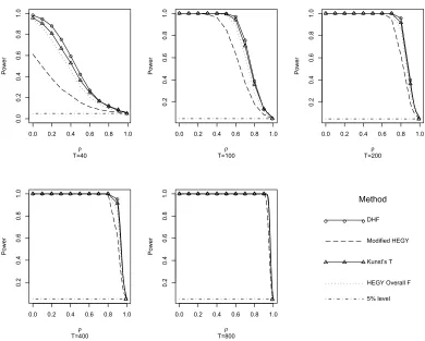
are stationary and 37 series are non-stationary) are generated to understand the prop-erties of the two multiple-step test procedures. According to the results of empirical power, which is the probability of rejecting the null when the null is not true, both multiple-step test procedures are superior to the DHF test but not much different from the Kunst t test and the HEGY test that combines the results of its subtests. According to the empirical sensitivity to the correct model, which is the conditional probability of choosing the right model given the null is rejected, the two-step test procedure is better than the three-step test procedure and it is asymptotically equiva-lent to the HEGY test. With the simulation results, we also discover some properties of the DHF, Kunst t and HEGY tests.

Chapter 4

The models in Chapter 2 assume that u_t in (1.2) is a white noise series. In Chapter 4, we extend our studies by allowingu_t to be a stationary AR(p₋4) (p >4) process. We focus on the case that u_t is a stationary AR(1) process and Y_t satisfies

Chapter 5

Chapter 2

A Comparison of Seasonal Unit

Root Test Criteria

2.1

Motivations and Modifications

The DHF test is a test of seasonal non-stationarity against a special seasonal stationarity. If only partial seasonal unit roots are present in Φ(B), its null and alternative hypotheses are both false. The results of Ghysels, Lee and Noh(1994) and Taylor (2003) imply that the DHF test has a non-zero probability of accepting the null hypothesis that the series admits all seasonal unit roots while the series only has partial seasonal unit roots. Taylor also provided large sample distributions of the DHF test statistics when the series is a random walk and thus validated that the DHF test can not distinguish between Y_t = Y_t−4 +ǫ_t and Y_t =Y_t−1+ǫ_t. To extend previous findings, we modify the HEGY model to test the presence of unit roots _±1 and _±i against the presence of unit roots _±1 only.

Consider the process

in (1.2). The polynomial Φ(B) for this process is

Φ(B) = 1₋αB2₋βB4 = (1₋B2)(1 +βB2),

and the roots of Φ(B) are

     

    

±1 and _±q₋1/β, β ₆= 0,1 (or α_∈(0,1)_∪(1,2)) ±1, β= 0 (or α= 1)

±1 and_±i, β= 1 (or α= 0)

To get a more intuitive expression, subtract Y_t−4 from both sides of (2.1):

Y_t−Y_t−4 =α(Y_t−2−Y_t−4) +u_t. (2.2)

It is trivial to see that the value of α in model (2.2) plays a critical role. When

α= 0, the process is generated by (1.2) and admits all four distinct unit roots; When

α_∈(0,2) (orα >0), the process is still nonsationary but only admits unit roots_±1. Consequently, the test of α = 0 against α > 0 is equivalent to the test of presence of roots _±1 and _±i against presence of roots _±1. It is obvious that model (2.2) is a reduced form of model (1.6). We call this test modified HEGY test throughout this study.

Unlike the DHF test, the modified HEGY test is a right tail test and does not allow testing against stationarity. An exploration of the properties of the DHF test statistics under the modified HEGY hypothesis can help us thoroughly understand why the DHF test does not have asymptotic power one when the series only has unit roots_±1. On the other hand, the modified HEGY model is a reduced HEGY model and the independent variables in the HEGY model are asymptotically independent. A study of the properties of the modified HEGY test can reveal the properties of the HEGY subtest on H₀₂.

introduced that Kunst’s model is a reparametrized HEGY model. From (1.9), it is trivial to find

        

       

θ₁ =λ₁₋λ₂₋λ₄;

θ₂ =λ₁+λ₂₋λ₃;

θ₃ =λ₁₋λ₂+λ₄;

θ₄ =λ₁+λ₂+λ₃.

λ’s are the coefficients in the HEGY model. λ₁ = 0, λ₂ = 0 and λ₃ = λ₄ = 0 are equivalent to the presence of root 1, -1 and _±i respectively. With the assumption

θ₁ =θ₂ =θ₃ = 0, (2.3)

θ₄ = 0 is equivalent to the presence of roots 1, -1 and _±i. θ₄ <0 implies that at least one of λ_i for i = 1,2,3 is less than zero and thus the corresponding H_0j (j = i₋1) and H₀ are rejected (see the definition of H_0j on page 7). According to these facts, we use the t-statistic to testθ₄ = 0 as the test statistic instead of using the F-statistic (F₁₂₃₄)to test θ₁ =θ₂ =θ₃ =θ₄ = 0. Although the t test may be not as powerful as the F test if the assumption (2.3) can not be ensured, the empirical results in Section 2.3 will show that τ_θ4=0 is usually preferred to F₁₂₃₄ for finite samples. In this study, the comparison betweenτ_θ4=0 andτ_ρ=1 (whereρis defined in (1.3)) is used to validate the significance of the additional variables, Y_t−1, Y_t−2 and Y_t−3. To be distinguished from the original Kunst test, the modified test is called Kunst’s t test in this paper.

2.2

Asymptotic Distributions

This section will provide and discuss the asymptotic distributions of the relative test statistics under the null hypothesis and the alternative hypotheses of the DHF and modified HEGY tests. The asymptotic distributions offer a good understanding of large sample behaviors for the tests under analysis.

2.2.1

Under the Null Hypotheses

To simplify the presentation, let _{u_t} in (1.2) be a white noise series, i.e. u_t =ǫ_t

and ǫ_{t ∼}i.i.d.(0, σ2_{). The series is a seasonal random walk and can be divided into}

four independent random walks:

        

       

X_1,n =Y_t =X_1,n−1+u_1,n and u_1,n =ǫ_t, mod(t,4) = 1;

X_2,n =Y_t =X_2,n−1+u_2,n and u_2,n =ǫ_t, mod(t,4) = 2;

X_3,n =Y_t =X_3,n−1+u_3,n and u_3,n =ǫ_t, mod(t,4) = 3;

X_4,n =Y_t =X_4,n−1+u_4,n and u_4,n =ǫ_t, mod(t,4) = 0.

For convenience, these X_i’s and u_i’s are used to derive the relevant asymptotic dis-tributions. In the following proofs, some asymptotic results from previous work are directly used without giving full proofs. These results are summarized in Appendix B. The number of observations for _{Y_t} is T = 4N and thus the size of _{X_i,n} for

i = 1,_{· · ·},4 is N. In this section, three scenarios for the deterministic components are considered: (1) zero mean; (2) seasonal means; (3) seasonal means and a single trend.

Scenario 1: Zero Mean Models

• N(ˆρ₋1) andˆτ_ρ=1

Let ˆρ and ˆτ_ρ=1 denote the estimator and t-statistic from model (1.3) withs = 4. The estimate ofρ₋1 in the DHF regression model is given by

ˆ

ρ₋1 =

P

Y_t−4(Y_t−Y_t−4)

P Y2

Under H₀, Y_t−Y_t−4 =ǫ_t, we have

ˆ

ρ₋1 =

P Y_t−4ǫ_t P

Y2 t−4

=

P

{X_1,n−1u_1,n+X_2,n−1u_2,n+X_3,n−1u_3,n+X_4,n−1u_4,n} P

{X2

1,n−1+X22,n−1+X32,n−1+X42,n−1}

= 1

N 1 N

P

{X_1,n−1u_1,n+X_2,n−1u_2,n+X_3,n−1u_3,n+X_4,n−1u_4,n} 1

N2

P

{X2

1,n−1+X22,n−1 +X32,n−1+X42,n−1}

From Lemma B.1 (see Appendix B), the asymptotic distribution forN(ˆρ₋1) is

N(ˆρ₋1)_→

P4 i=1

R1

0 Wi(t)dWi P₄

i=1 R₁

0 Wi2(t)dt

, (2.4)

where W_i(t) _∼ N(0, t) and are independent of W_j(t) if i ₆= j, and we use “_→” to denote convergence in distribution throughout this chapter. The sample t-statistic for testingρ = 1 is calculated by

ˆ

τ_ρ=1 = q ρˆ−1

ˆ

σ2_/P

{X2

1,n−1 +X22,n−1+X32,n−1+X42,n−1}

=

1 N

P

{X_1,n−1u_1,n+X_2,n−1u_2,n+X_3,n−1u_3,n+X_4,n−1u_4,n} q

1 N2ˆσ2

P

{X2

1,n−1+X22,n−1+X32,n−1+X42,n−1} ,

where ˆσ2 ₌ 1 T−2

P

(Y_t−ρYˆ _t−4)2 _→P _σ2 _{and “→}P _{” denotes convergence in probability}

throughout this chapter. With the results from (2.4), it is easy to see that,

ˆ

τ_ρ=1→ P4

i=1 R1

0 Wi(t)dWi q

P4 i=1

R₁

0 Wi2(t)dt

(2.5)

• Nθˆ₄ and ˆτ_θ4=0

asymptotically orthogonal, it is relatively simple to derive the asymptotic behavior of ˆθ₄ from the asymptotic results of the HEGY estimates.

According to the comparison between the HEGY reparametrization model shown in (1.9) and Kunst’s model, it is easy to observe that λ₁+λ₂+λ₃ = θ₄. The linear relation betweenθ’s andλ’s implies that the OLS estimate, ˆθ₄, can be obtained by the sum of the OLS estimates, ˆλ₁, ˆλ₂ and ˆλ₃. The asymptotic distributions of Nθˆ₄ and ˆ

τ_θ4=0 can be derived from the asymptotic results given by Beaulieu and Miron (1992). In particular, when s= 4, the asymptotic results forNλˆ’s and the corresponding ˆτ’s are                                 

Nλˆ_{1 →} 4 R1

0 B1(t)dB1

16R₀1B2 1(t)dt

, τˆ_{λ1 →}

R1

0 B1(t)dB1

q R1

0 B 2 1(t)dt

Nλˆ_{2 →} 4 R1

0 B2(t)dB2

16R₀1B2 2(t)dt

, τˆ_{λ2 →}

R1

0 B2(t)dB2

q R1

0 B 2 2(t)dt

Nλˆ_{3 →} 2 _R1

0 B3(t)dB3+

R1

0 B4(t)dB4

4R₀1(B2

3(t)+B42(t))dt

, τˆ_{λ3 →}

R1

0 B3(t)dB3+

R1

0 B4(t)dB4

[R₀1(B2

3(t)+B42(t))dt]1/2

Nλˆ_{4 →} 2 _R1

0 B4(t)dB3−

R1

0 B3(t)dB4

4R₀1(B2

3(t)+B42(t))dt

, τˆ_{λ4 →}

R1

0 B4(t)dB3−

R1

0 B3(t)dB4

[R₀1(B2

3(t)+B42(t))dt]1/2

B_i(t)_∼N(0, t) and are defined as the following functions of W_i’s:

                

B₁(t) = 1

2(W1(t) +W2(t) +W3(t) +W4(t)) B₂(t) = 1

2(−W1(t) +W2(t)−W3(t) +W4(t)) B₃(t) = _√1

2(W2(t)−W4(t)) B₄(t) = _√1

2(W1(t)−W3(t))

With the construction of the HEGY variables, the cross product of the resulting design matrix is asymptotically orthogonal when normalized by N2_{. Consequently,}

the variance of ˆθ₄ is approximately the sum of variances of ˆλ₁, ˆλ₂ and ˆλ₃, and the asymptotic distributions for Nθˆ₄ and its t-statistic are

Nθˆ_{4 →} 4 R₁

0 B1(t)dB1

16R1

0 B12(t)dt

+ 4

R₁

0 B2(t)dB2

16R1

0 B22(t)dt

+ 2

R₁

0 B3(t)dB3+ R₁

0 B4(t)dB4

4R1

0(B32(t) +B42(t))dt

and

ˆ

τ_{θ4=0 →}  



4R₀1B1(t)dB1

16R₀1B2 1(t)dt

+4

R1

0 B2(t)dB2

16R₀1B2 2(t)dt

+ 2

R1

0 B3(t)dB3+

R1

0 B4(t)dB4

4R₀1(B2

3(t)+B42(t))dt

 



×qR₁

0(16B12(t) + 16B22(t) + 4B23(t) + 4B42(t))dt

(2.7)

• Nαˆ and ˆτ_α=0

ˆ

α and ˆτ_α=0 are estimator and t-statistic in the regression model (2.2). The OLS estimate ˆα in the modified HEGY model can be obtained by

ˆ

α=

P

(Y_t−2−Y_t−4)(Y_t−Y_t−4)

P

(Y_t−2−Y_t−4)2

With the assumption that Y_t is generated by Y_t=Y_t−4+ǫ_t, ˆα is equal to

ˆ

α =

P

(Yt−2−Yt−4)ǫt

P

(Yt−2−Yt−4)2 =

=

P

{(X1,n−X3,n−1)u3,n+(X2,n−X4,n−1)u4,n+(X3,n−1−X1,n−1)u1,n+(X4,n−1−X2,n−1)u2,n}

P

{(X1,n−X3,n−1)2+(X2,n−X4,n−1)2+(X3,n−1−X1,n−1)2+(X4,n−1−X2,n−1)2}

According to Lemma B.2 in Appendix B, the numerator isO_p(N). When divided by N, the numerator will converge as follows:

1

N

P

{(X1,n−X3,n−1)u3,n+ (X2,n−X4,n−1)u4,n+ (X3,n−1−X1,n−1)u1,n+ (X4,n−1−X2,n−1)u2,n}

→R₀1W1(t)dW3+

R1

0 W2(t)dW4+

R1

0 W3(t)dW1+

R1

0 W4(t)dW2−

P4

i=1

R1

0 Wi(t)dWi;

moreover, the denominator converges at rateN2_: 1

N2

P

{(X_1,n−X_3,n−1)2_{+ (X}

2,n−X4,n−1)2+ (X3,n−1−X1,n−1)2+ (X4,n−1−X2,n−1)2} →2_{R1

0(W1(t)−W3(t))2dt+ R1

0(W2(t)−W4(t))2dt}

Combine the limits of both denominator and numerator:

Nαˆ _→

R1

0 W1(t)dW3+ R1

0 W2(t)dW4+ R1

0 W3(t)dW1+ R1

0 W4(t)dW2−P4i=1 R1

0 Wi(t)dWi

2_{R₁

0(W1(t)−W3(t))2dt+ R₁

0(W2(t)−W4(t))2dt