KEISLTER, PATRICK G. Simulation of Supersonic Combustion Using Variable Turbulent Prandtl/Schmidt Numbers Formulation. (Under the direction of Dr. Hassan A. Hassan.)
A turbulence model that allows for the calculation of the variable turbulent Prandtl (Prt) and Schmidt (Sct) numbers as part of the solution is presented. The model
also accounts for the interactions between turbulence and chemistry by modeling the corresponding terms. Four equations are added to the baseline k-ζ turbulence model: two equations for enthalpy variance and its dissipation rate to calculate the turbulent diffusivity, and two equations for the concentrations variance and its dissipation rate to calculate the turbulent diffusion coefficient. The variable Prt/Sct turbulence model is
used to simulate the SCHOLAR supersonic combustion experiments. The experiments include one model with normal hydrogen injection into a vitiated airstream at Mach 2.0, while the other injects hydrogen at Mach 2.5 and an angle of 30° to the vitiated airstream. Two sets of calculations are presented for each experiment, one where the turbulent Prandtl and Schmidt numbers are constant and one where they are allowed to vary. Two chemical kinetic models are employed for each calculation: a seven species/seven reaction model where the reaction rates are temperature dependent and a nine species/nineteen reaction model where the reaction rates are dependent on both pressure and temperature.
The simulation of the vectored injection experiment predicts an earlier ignition than what is suggested by the experimental data. Also, the downstream pressure is underpredicted. The temperature distribution in the downstream portion of the combustor is higher with the variable Prt/Sct model than with the constant model, which places it
Simulation of Supersonic Combustion Using Variable
Turbulent Prandtl / Schmidt Numbers Formulation
by
Patrick Keistler
A thesis submitted to the Graduate Faculty of North Carolina State University
in partial fulfillment of the requirements for the Degree of
Master of Science
Mechanical and Aerospace Engineering
Raleigh, North Carolina
2006
Approved by:
___________________________ ___________________________ Jack R. Edwards D. Scott McRae
___________________________ Hassan A. Hassan
Biography
Acknowledgements
Table of Contents
List of Figures ... vi
List of Tables ... viii
List of Symbols ... ix
1 Introduction... 1
2 Governing Equations ... 5
2.1 Reacting Gas Equation Set... 5
2.1.1 Navier-Stokes Equations... 5
2.1.2 Thermodynamic Relations ... 7
2.2 Governing Equations in Vector Form... 8
2.3 Reynolds and Favre Averaging... 9
2.4 Chemical Kinetics ... 11
2.4.1 Jachimowski Chemical Mechanism... 13
2.4.2 Connaire et al. Chemical Mechanism ... 13
2.5 Turbulence Closure ... 15
2.5.1 k-ζ Model ... 16
2.5.2 Variable Turbulent Prandtl Number Model ... 19
2.5.3 Variable Turbulent Schmidt Number Model ... 22
2.5.4 Turbulence / Chemistry Interactions... 25
2.6 Complete Equation Set ... 26
2.6.1 Solution Methods ... 26
3 Experimental Overview ... 27
3.1 The SCHOLAR Experiments ... 27
3.1.1 Vectored Injection Case ... 28
3.1.2 Normal Injection Case ... 30
3.2 CARS Measurement Techniques ... 32
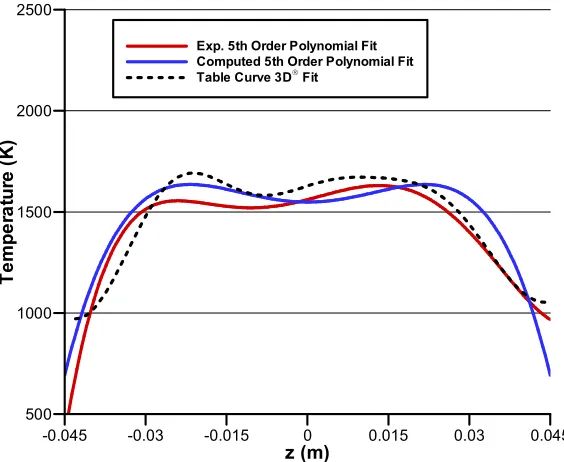
3.3 Experimental Data Fitting... 33
4 Implementation ... 35
4.2 Computational Geometry... 35
4.3 Wall and Inlet Boundary Conditions ... 39
4.3.1 Wall Boundaries... 39
4.3.2 Inflow and Outflow Boundaries... 41
5 Results and Discussion ... 42
5.1 General Results ... 42
5.2 Vectored Injection Model ... 47
5.2.1 Variable Prt / Sct Runs ... 47
5.2.2 Constant Prt / Sct Runs ... 56
5.3 Normal Injection Model... 60
5.3.1 Constant Prt / Sct Run ... 61
5.3.2 Variable Prt / Sct Run ... 64
6 Conclusions... 71
References... 73
Appendix A: Governing Equations Vectors ... 78
Appendix B: Transformation to Generalized Coordinates ... 80
Appendix C: Chemical Kinetic Mechanism Parameters ... 84
Appendix D: Complete Equation Set in Vector Form ... 88
List of Figures
Figure 3.1: Schematic of Vectored Injection SCHOLAR Experiment... 28
Figure 3.2: Detail of Vectored Hydrogen Injector... 29
Figure 3.3: Schematic of Normal Injection SCHOLAR Experiment ... 30
Figure 3.4: Detail of Normal Hydrogen Injector ... 31
Figure 3.5: Example of CARS Measurements and Curve Fit (Plane 6, y = 18.2 mm)... 34
Figure 4.1: Block Layout and H2 Injector Detail for Vectored Injection ... 36
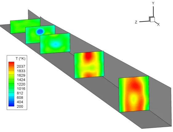
Figure 4.2: Vectored Block Layout with CARS Survey Planes Highlighted ... 37
Figure 4.3: Block Layout and H2 Injector Detail for Normal Injection... 38
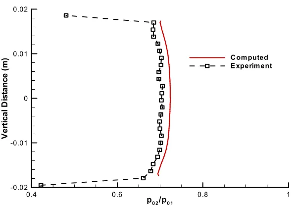
Figure 5.1: Pitot Pressure Profile at Vitiated Air Nozzle Exit... 44
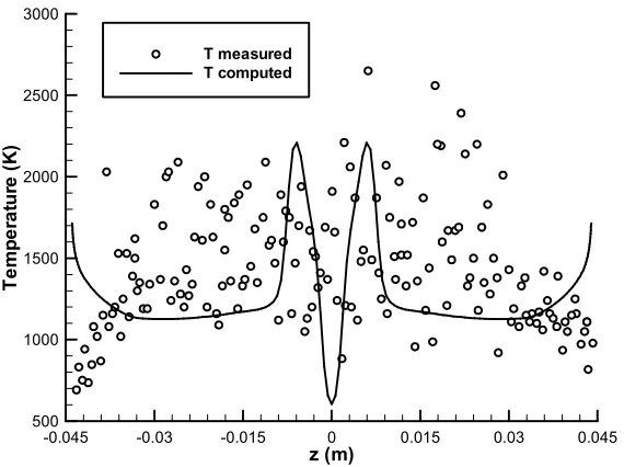
Figure 5.2: Temperature Slice with Adiabatic Wall Temperature... 45
Figure 5.3: Wall Temperature vs. Run Time at Three Locations (Ref [11]) ... 46
Figure 5.4: Temperature Slice of Plane 6 at y = 18.2 mm (Connaire)... 48
Figure 5.5: Mole Fraction Slices of Plane 6 at y = 18.2 mm (Connaire)... 49
Figure 5.6: 5th Degree Polynomial Fits of Exp. and Computed Temperature (Run 1) ... 50
Figure 5.7: 5th Degree Polynomial Fits of Exp. and Computed Mole Fractions (Run 1) . 50 Figure 5.8: Experimental Surface Fits of Temperature for Vectored Case ... 51
Figure 5.9: Temperature Contours for Run 1... 52
Figure 5.10: Nitrogen and Oxygen Mole Fractions for Run 1... 52
Figure 5.11: Temperature from Runs 1 and 2 (Left: Jach., Right: Connaire)... 53
Figure 5.12: Wall Pressures for Runs 1 and 2 ... 54
Figure 5.13: OH Mole Fractions for Runs 1 and 2 (Left: Connaire, Right: Jach.) ... 55
Figure 5.14: Turbulent Prantl Number (left) and Turbulent Schmidt Number (right) ... 56
Figure 5.15: Temperature Contours for Run 3... 57
Figure 5.16: Nitrogen and Oxygen Mole Fractions for Run 3... 58
Figure 5.17: Temperature from Runs 3 and 4 (Left: Jach., Right: Connaire)... 59
Figure 5.18: Wall Pressures for Runs 3 and 4 ... 60
Figure 5.20: Mole Fraction Contours for Run 5 (left: N2, right: O2) ... 62
Figure 5.21: Bottom Wall Pressure for Run 5 ... 63
Figure 5.22: Temperature Contours for Run 6... 64
Figure 5.23: Mach Contours on Symmetry Plane for Run 6 ... 65
Figure 5.24: Mach Contours on Symmetry Plane for Run 5 ... 66
Figure 5.25: Mole Fraction Contours for Run 6 (left: N2, right: O2) ... 67
Figure 5.26: Bottom Wall Pressure for Runs 5 and 6 ... 67
Figure 5.27: 3D Hydrogen Mole Fraction Contours for Run 6 ... 68
Figure 5.28: Stream Traces Originating in Hydrogen Injector ... 69
List of Tables
Table 2.1: Troe Parameters for Connaire et al. Mechanism ... 15
Table 2.2: k-ζ Model Closure Coefficients ... 19
Table 2.3: Variable Prandtl Number Model Constants... 22
Table 2.4: Variable Schmidt Number Model Constants... 25
Table 3.1: Inflow Conditions for Vectored Injection... 30
Table 3.2: Inflow Conditions for Normal Injection ... 32
Table 5.1: Runs Presented... 47
Table C.1: Abridged Jachimowski Mechanism Reactions ... 84
Table C.2: Abridged Jachimowski Mechanism Parameters ... 84
Table C.3: Connaire et al. Mechanism Reactions... 85
Table C.4: Connaire et al. Mechanism Parameters... 86
List of Symbols
Roman Symbols:
A Pre-exponential factor / face area A – G Euler Implicit matrix coefficients
a Speed of sound
a,T*,T**,T*** Fall-off reaction rate constants
a1,m – b1,m Thermodynamic curve fit coefficients Ch – βh Variable Prandtl number model constants Cm Species concentration
Cmix Mixture concentration
Cp Specific heat ratio at constant pressure
Cp,mix Mixture specific heat ratio at constant pressure CY – βY Variable Schmidt number model constants Cµ – Cζ1 k-ζ model closure coefficients
D Binary diffusion coefficient Dt Turbulent diffusion coefficient
E Total energy
Ea Activation energy G
F E
r r r
,
, x, y, and z direction inviscid fluxes G
F
Eˆ, ˆ, ˆ ξ, η, and ζ direction inviscid fluxes G
F
E~, ~, ~ Average interface fluxes
v v v F G E
r r r
,
, x, y, and z direction viscous fluxes
v v v F G
Eˆ , ˆ , ˆ ξ, η, and ζ direction viscous fluxes em Species internal energy
emix Mixture internal energy F Fall-off reaction rate function
F r
Flux vector
gˆ Gibbs free energy per mole
H Total enthalpy
~
2
h′′ Enthalpy variance
∆hf,m Species heat of formation hm Species enthalpy
m
hˆ Species enthalpy per mole hmix Mixture enthalpy
J Transformation Jacobian
k0 Low pressure reaction rate coefficient
kb,i Backward reaction rate coefficient
keq|C Equilibrium constant based on concentrations
keq|P Equilibrium constant based on partial pressures
kf,i Forward reaction rate coefficient km Species thermal conductivity
k∞ High pressure reaction rate coefficient
M Mach number
Mt Turbulent Mach number
m’,m” Forward and backward reaction order
i
x
nˆ Cell face normal vector
Pr Prandtl number
Prt Turbulent Prandtl number
p Pressure
pm Species partial pressure pr Reduced pressure
Qj Turbulent heat flux vector qj Heat flux vector
R r
Residual vector Rˆ Universal gas constant Rmix Mixture gas constant RRi Reaction rate
±
r Adjacent slope ratios S
S, ˆ r
Source vector
Sc Schmidt number
Sct Turbulent Schmidt number
sij Instantaneous strain rate tensor
T Temperature
Tij Reynolds stress tensor TBm,j Species third body efficiency Tu Turbulence intensity
t Time
U U, ˆ
r
Conservative variable vector
C C C V W
U~ ,~ , ~ Contravarient velocities
m m m V W
U~ , ~ , ~ Species contravarient velocities ui Cartesian velocity in index notation u,v,w Cartesian velocity components
V Cell volume
Vm,j Species diffusion velocityin index notation m
Wˆ Species molecular weight x,y,z Cartesian coordinates
~
2Y ′′ Mass fraction variance Ym Species mass fraction
Ym,j Turbulent species diffusion vector
Greek Symbols:
α Thermal diffusivity
αt Turbulent thermal diffusivity
∆ Different operator δij Kronecker delta
εh Dissipation rate of enthalpy variance εijk Permutation tensor
εY Dissipation rate of σY γmix Mixture specific heat ratio
η Temperature exponent
κ Parameter used in kappa scheme
µ Molecular viscosity
µm Species molecular viscosity µt Turbulent viscosity
ν Kinematic viscosity
νt Turbulent kinematic (eddy) viscosity i
m i m,,ν ,
ν′ ′′ Species reactant and product stoichiometric coefficients θd Activation temperature
ρ Density
ρm Species density σ System spectral radius
σY Sum of mass fraction variances τij Laminar stress tensor
ωi Vorticity vector m
ω
& Species production rateξ,η,ζ Generalized Coordinate Directions
i i
i x x
x
η
ζ
ξ
, , Metric derivatives in index notationΨ Limiter function
ζ Vorticity variance (enstrophy)
Subscripts:
b Backward
C Contravariant
CV Control volume
E Edwards (LDFSS)
eq Equilibrium
i,j,k Grid indices / index notation 2
1 2 1 2
1, + , +
+ j k
i Cell faces
L Left
m Species
mix Mixture property
NS Number of species
R Right
t Turbulent
V Viscous
VL van Leer
w Wall
∞ Freestream
Superscripts:
C Convective
I Inviscid
n Time step
P Pressure
Accents:
– Reynolds averaged
~ Favre averaged / average interface flux
^ Per mole
. Time rate of change
‘ Reynolds fluctuation / reactants “ Favre fluctuation / products
Abbreviations:
CARS Coherent anti-Stokes spectroscopy CFD Computational Fluid Dynamics CFL Courant Freidrichs and Lewy DNS Direct numerical simulation ENO Essentially non-oscillatory ILU Incomplete Lower Upper
LDFSS Low diffusion flux splitting scheme LES Large eddy simulation
MPI Message Passing Interface PDF Probability density function RANS Reynolds averaged Navier-Stokes TVD Total variation diminishing
Other symbols:
∂ Partial derivative
1
Introduction
Some efforts have been made to move toward the calculation, rather than specification, of the turbulent Prandtl and Schmidt numbers as part of the solution. Methods based on the mixing length have been employed as early as 1975, by Reynolds, to calculate both the turbulent Prandtl and Schmidt numbers [30]. In 1988, Nagano developed a two equation model for calculating the turbulent diffusivity, which was used in conjunction with the k-ε turbulence model [28]. However, the model was not developed for high speed flow and thus does not include the effects of compressibility. This model provided the framework for most of the work to follow. In 1993, Sommer et al. developed a variable turbulent Prandtl number model using methods very similar to those used by Nagano [35]. This model was also derived from the incompressible energy equation rather than the compressible energy equation, so compressibility effects, which have been determined to be quite important, are not accounted for. Two additional equations were added to the base incompressible k-ε turbulence model, temperature variance, and its dissipation rate. Solving these four equations allowed for the calculation of the turbulent diffusivity. In general the results for high Mach number, low wall temperature cases were improved over those utilizing the k-ε model alone. In 1999, another approach was taken by Guo et al. to create a variable turbulent Schmidt number model [18]. In addition to the k-ε turbulence model, Guo modeled the turbulent species diffusion vector with a single transport equation. A genetic algorithm technique was applied to efficiently obtain the model constants. Again, the results were improved over the baseline k-ε model for a jet-in-crossflow application.
was later applied by CRAFT Tech to a Large Eddy Simulation (LES) of reacting and non-reacting shear layers at high speeds [6][7]. The purpose of this work was to generate data to be used in improving RANS models. Compressibility corrections were applied in this work, but the model constants were modified in an ad hoc manner, without significant validation. The model was extended to include variable Prt and variable Sct in
2005 [4].
In 2005, Xiao et al. presented two similar approaches, one for calculating the turbulent Prandtl number (Prt) as part of the solution [42] and one for calculating the
turbulent Schmidt number (Sct) as part of the solution [41]. Each of these new models
used the k-ζ turbulence model of Robinson and Hassan as a base [31]. With the addition of two equations each, enthalpy variance and its dissipation rate for the variable Prt model
and concentrations variance and its dissipation rate for the variable Sct model, the
turbulent diffusivity and the turbulent diffusion coefficient were able to be determined. Improvements were observed for a coaxial jet flow [9] with the variable Sct model, and
improvements in heat flux predictions were seen with the variable Prt model. The
variable Sct model was later applied to the supersonic combustion experiment of Burrows
and Kurkov [5], while using a probability density function (PDF) to address the turbulence/chemistry interactions. In general the variable Sct formulation worked well
for both mixing and reacting supersonic flows; however, the PDF method for addressing turbulence/chemistry interactions did not necessarily improve the results [22]. A complete turbulence model, where both the Prt and Sct are calculated as part of the
The SCHOLAR combustor has been simulated extensively by Rodriguez and Cutler in conjunction with the actual experiments. Initially, only mixing was considered [13], then the reacting case [10]. Rodriguez and Cutler later continued the work in a more comprehensive study [33]. The simulation utilized the VULCAN CFD code, developed at NASA Langley Research Center. The k-ω turbulence model was used with various constant values of Prt and Sct. The computed results were seen to vary greatly
with the specification of these parameters. The best results were obtained with Prt = 0.9
and Sct = 1.0, therefore, the constant Prt/Sct runs in the current work use these values.
2
Governing Equations
This section will describe the set of partial differential equations that governs the physics of supersonic multi-component reacting gasses.
2.1
Reacting Gas Equation Set
2.1.1
Navier-Stokes Equations
The governing equations for multi-component compressible chemically reacting flows at high speeds are the Navier-Stokes equations, which consist of conservation of mass, momentum, and energy, along with a set of species mass conservation equations. The number of species equations required is NS – 1, where NS is the number of species. By including all of the species equations, the continuity equation may be removed, since the sum of the species mass conservation equations results in the continuity equation. If external forces such as gravity, and body forces are neglected, and thermal equilibrium is assumed, the equations are as follows:
( )
=0∂ ∂ + ∂ ∂
i i
u x
t ρ
ρ
(2.1)
( )
(
+ −)
=0∂ ∂ + ∂
∂
ij ij j i j
i uu p
x u
t
ρ
ρ
δ
τ
(2.2)( )
(
+ −)
=0∂ ∂ + ∂
∂
i ij j j j
u q Hu x E
t
ρ
ρ
τ
(2.3)(
)
(
m j m jm)
mj
m Y u Y V
x Y
t
ρ
ρ
ρ
ω
&
= +
∂ ∂ + ∂
∂
In these equations, ρ is the density, ui is the velocity, p is the pressure, τij is the stress
tensor, and qj is the heat flux vector. For the species mass conservation equations, Ym is
the species mass fraction, Vj,m is the diffusion velocity, and w&m is the production rate.
The viscous stress tensor, under the assumption of a Newtonian fluid, can be written as
k k ij ij ij
x u s
∂ ∂ −
=
µ
δ
µ
τ
3 2
2 (2.5)
∂ ∂ + ∂ ∂ =
i j
j i ij
x u x u s
2 1
(2.6)
where µ is the molecular viscosity and sij is the instantaneous strain rate tensor. The heat
flux vector is evaluated using the sum of Fourier’s Law and the heat flux due to diffusion.
∑
=+ ∂ ∂ −
= NS
m
i m m m i
i h Y V
x T k q
1
,
ρ (2.7)
Similar to the viscous stress and heat flux, a linear relationship can be developed for the species diffusion mass flux. This is called Fick’s Law [26], and it states that the diffusion mass flux is proportional to the species concentration gradients.
i m m i
m
x Y Y
D V
∂ ∂
=ρ
ρ , (2.8)
The binary diffusion coefficient, D, is defined by the Schmidt number (Sc).
D ρ
µ
=
Sc (2.9)
The total energy and total enthalpy are defined by the following equations.
ρ p H
E= − (2.10)
2
i i mix
u u h
H = + (2.11)
The mixture specific enthalpy is defined by a mass fraction weighted sum.
∑
== NS
m m m mix Y h
h
1
The species enthalpies, hm, will be defined in Section 2.1.2. The equation of state is used
to relate the pressure, bulk density, and temperature. It is known as Dalton’s Law of Partial Pressures.
T R p
p mix
NS
m
m =ρ
=
∑
=1
(2.13)
This law states simply that the pressure is the sum of the partial pressures of each species.
∑
== NS
m m m mix
W Y R R
1 ˆ
ˆ (2.14)
m
Wˆ is the molecular weight of species m, and Rˆ is the universal gas constant. The total energy can also be written in the form of Equation (2.11).
2
i i mix
u u e
E = + (2.15)
The mixture internal energy, emix, is also defined in terms of the species enthalpies.
∑
∑
− =
=
= m
m m NS
m m m mix
W T R h Y e
Y e
ˆ ˆ
1
(2.16)
2.1.2
Thermodynamic Relations
For a high temperature, chemically reacting flow, the flow is assumed to be thermally perfect. Unlike the assumptions of a calorically perfect gas, the specific heats at constant pressure and volume are no longer assumed constant. They are instead functions of temperature. A thermally perfect gas is based on the assumption that the internal energy modes of a molecule are always in a state of equilibrium. Curve fits given in [27] are used to calculate the specific heats along with other related properties. The species enthalpy can easily be obtained from these curve fits using the following equation.
T b T a T a T a T a a T R
h m
m m
m m
m
m 4 1,
, 5 3
, 4 2
, 3 ,
2 , 1
5 4
3 2
ˆ ˆ
+ +
+ +
+
The species enthalpy in this equation is defined on a per mole basis. To obtain the enthalpy per unit mass, simply multiply by the species molecular weight. Specific heat, entropy, and Gibbs free energy can be calculated in a similar manner.
The ratio of specific heats for the mixture, γmix, can be calculated using:
mix p
p mix
R C
C
mix mix
− =
γ
(2.18)∑
== NS
m p m pmix Y C m
C
1
(2.19)
Finally, the laminar viscosity and thermal conductivity must be determined. First the laminar viscosity for each species is calculated using Sutherland’s Law [38]. The laminar thermal conductivity is then calculated from the following relation to the laminar Prandtl number.
Pr
m
p m m
C
k = µ (2.20)
Then, using Wilke’s formula [26], the species viscosities and thermal conductivities are combined into a bulk or mixture viscosity and thermal conductivity.
2.2
Governing Equations in Vector Form
A convenient way to rewrite the Navier-Stokes equations is in compact vector form. This makes further formulations much simpler. The general form is as follows.
(
) (
)
(
)
S z
G G y
F F x
E E t
U v v v r
r r r
r r
r r
= ∂
− ∂ + ∂
− ∂ + ∂
− ∂ + ∂ ∂
(2.21)
2.3
Reynolds and Favre Averaging
While the Navier-Stokes equations describe continuum fluid flow down to the smallest scales of turbulent motion, the discrete computational grids on which the equations are solved are unable to resolve such small scales of motion. The small turbulence scales are very important however, in dissipating energy from larger scale motion and the mean flow. The traditional approach to this problem is not to resolve the smallest features of the flow, but rather to model them using the local characteristics and time history of the flow. This provides a macroscopic view of the affects of turbulence on the mean flow.
There are certainly alternatives to modeling the turbulence. One such alternative is direct numerical simulation (DNS), in which the exact Navier-Stokes equations are resolved down to the smallest turbulence scales. This requires many times more grid points than a solution where the turbulence is completely modeled, and the requirement is ever steeper with increasing Reynolds numbers. Another alternative is to resolve some of the large scale turbulent features and model the scales that occur on the sub-grid level. This is known as large eddy simulation (LES). This is a compromise, but it still requires a significantly higher resolution than simulations that model all turbulence scales. Due to the size of modern engineering problems and the limited computing power that is available, a completely modeled approach is adopted in the current work.
A method called Reynolds averaging is used to convert the governing equations to solve for the mean flow properties rather than the instantaneous properties. There are a number of ways to average the flow properties, but for stationary turbulence, such as that in steady flows, time averaging is the most appropriate [40]. The following equation represents this time averaging process.
(
)
∫
+∞ →
= t T
t i
T i
T f x t dt
T x
The instantaneous flow property is represented by f(xi,t) while FT(xi) is the time averaged
flow property. The instantaneous flow properties can then be expressed by the time averaged mean property plus a fluctuation.
q q
q= + ′ (2.23)
Here, q represents any flow property; q is the time averaged quantity and q′ is the fluctuation. This averaging is applied to the velocity and pressure fluctuations.
Applying this time averaging technique to the Navier-Stokes equations results in what is known as the Reynolds Averaged Navier-Stokes (RANS) equations. While this method works well for incompressible flows, more variables must be taken into account if the flow is compressible, namely density and temperature. However, if the same Reynolds averaging technique is used, terms arise that have no analogue to those in the incompressible equations. To alleviate this problem, a different type of averaging is introduced, Favre, or mass-weighted averaging. This average is obtained from the following equation.
(
) (
)
∫
+∞ →
= t T
t i i
T x t q x t dt
q~ 1 lim ρ , ,
ρ (2.24)
Here, q~ represents the Favre averaged quantity, and, just as before, the instantaneous quantity can be written as:
q q
q=~+ ′′ (2.25)
When averaging the equations, correlation terms appear that are not necessarily zero. Consider the averaging of the product of any two variables.
(
ϕ ϕ)(
ψ ψ)
ϕψ ϕψ ψϕ ϕψ ϕψ ϕψϕψ = + ′ + ′ = + ′+ ′+ ′ ′= + ′ ′ (2.26)
The terms with only one fluctuating term become zero when averaged, but the product of two fluctuating properties is not necessarily zero if there is a correlation between them. The density, pressure, stress tensor, heat flux, and species production rate are represented using the Reynolds average, while the other variables use the Favre average.
m m m i i i
ij ij ij q
q q
p p p
ω
ω
ω
τ
τ
τ
ρ
ρ
ρ
′ + = ′
+ =
′ + = ′
+ = ′ + =
& & &
,
, ,
,
T T T H H H E E E Y Y Y V V V u u
ui i i im im im m m m
′′ + = ′′ + = ′′ + = ′′ + = ′′ + = ′′ + = ~ , ~ , ~ , ~ , ~ , ~ , , , (2.28)
Substituting these quantities into the Navier-Stokes equations and performing the prescribed averaging results in the Favre averaged Navier-Stokes equations, still known as the RANS equations [43].
(
~)
=0∂ ∂ + ∂ ∂ i i u x t ρ ρ (2.29)
( )
(
)
m j mj m j m j j
m Y u
x Y D x Y u x Y
t
ρ
ρ
ρ
ρ
ω
& + ′′ ′′ − ∂ ∂ ∂ ∂ = ∂ ∂ + ∂ ∂ ~ ~ ~ ~ (2.30)
(
)
(
)
[
ij j i]
j i i
j j
i u u
x x p u u x u
t ∂ − ′′ ′′
∂ + ∂ ∂ − = ∂ ∂ + ∂ ∂
ρ
~ρ
~ ~τ
ρ
(2.31)( )
(
)
[
(
)
]
(
q uh)
x u u u x u H x E
t i i i j ij j i ∂ i i + i′′ ′′
∂ − ′′ ′′ − ∂ ∂ = ∂ ∂ + ∂ ∂
ρ
~ρ
~~τ
ρ
ρ
(2.32)Three new terms are introduced in this form of the equations, the turbulent stress tensor,
i ju
u′′ ′′
−
ρ
, the turbulent heat flux vector,ρ
uih′′ ′′, and the turbulent species diffusionvector, −
ρ
Ym′′uj′′. These terms are approximated by the turbulence model to be defined in Section 2.5. The turbulent stress tensor is also known as the Reynolds stress tensor.2.4
Chemical Kinetics
A chemical mechanism consists of a collection of exchange/recombination reactions and third body reactions, which when combined, result in the global reaction such as that for hydrogen oxidation. The Law of Mass Action for exchange/recombination reactions is:
∏
∏
= ′′
= ′
−
= NS
m m i b NS
m m i f i
i m i
m k C
C k
RR
1 , 1
,
,
, ν
ν
(2.33)
For third body reactions, which require any third molecule to initiate, the equation becomes:
−
=
∏
∏
∑
= =
′′
=
′ NS
m
i m m NS
m m i b NS
m m i f
i k C k C C TB
RR mi mi
1
, 1
, 1
,
,
, ν
ν
(2.34)
Cm is the species concentration, or molar density, which is the species density divided by
the molecular weight. The stoichometric coefficients for the reactants are designated by ν’ and for the products, ν”. The effects of the third body are combined into a single term called the third body efficiency, TBm,i. Each species has a third body efficiency for each
third body reaction. The forward reaction rate coefficient, kf,i, is determined by the
Arrhenius Law. It takes the following form.
) / exp( T AT
kf = η −
θ
d (2.35)The parameters A, η, and θd are specific to the chemical kinetic mechanism and will be
discussed in Sections 2.4.1 and 2.4.2. Rather than require a separate set of parameters for the backward rate coefficient, kb is calculated using the equilibrium coefficient with the
following relation.
) (
ˆ
101325 m m
P eq C eq b f
T R k
k k
k ′′− ′
=
= (2.36)
The above equation also demonstrates the conversion of the equilibrium constant from a partial pressure basis to a concentration basis, as indicated by the subscripts. The equilibrium constant for a particular reaction can be calculated from the change in Gibbs free energy.
∆−
=
T R
g k
P
eq ˆ
ˆ
∑
′′ − ′ =∆ NS
m
m m
m g
gˆ (
ν
ν
)ˆ (2.38)The production rate of each species can be determined using the preceding information.
m NR
i
i i m i m
m ( )RR Wˆ
1
,
,
′′ − ′
=
∑
=
ν
ν
ω
& (2.39)2.4.1
Jachimowski Chemical Mechanism
The abridged chemical kinetic mechanism of Jachimowski is one of two models used in this work [21]. The mechanism consists of seven species and seven reactions. The species are N2, O2, H2, H2O, OH, H, and O. The reactions are listed in Table C.1 of
Appendix C. Note that the first two reactions are third body reactions, where M represents the third body. Thus, each equation requires a third body (TB) efficiency for each species. The species H2 has TB = 2.5 for both reactions and H2O has TB = 16.0 for
both reactions. All other species have a third body efficiency of 1.0 for both reactions. The mechanism parameters, such as the pre-exponential factor and activation energies are listed in Table C.2.
2.4.2
Connaire et al. Chemical Mechanism
method for computing the forward rate constant. While the classic definition of the rate constant is a function of the temperature, many chemical reactions are also a function of the pressure. Reactions 9 and 15 are examples of this. At very high pressures the rate constant may be defined by one set of parameters and at very low pressures by another set of parameters, and some blend of the two in between. This is known as a “fall-off” rate constant [26]. The ‘A’ and ‘B’ portions of reactions 9 and 15 represent the lower and upper pressure bounds respectively. A method presented by Troe et al. is used to blend these two limiting cases for intermediate pressures [17]. Using the two sets of parameters specified for the equation, a high-pressure limit rate constant, k∞, and a low-pressure limit
rate constant, k0, are determined. The final forward rate constant is determined from the
following equation.
F p p k k
r r
+
= ∞
1 (2.40)
The reduced pressure, pr, is related to the concentration of the mixture.
∞
=
k C k
p mix
r
0 (2.41)
The mixture concentration can be determined by dividing the bulk density by the molecular weight of the mixture. The function F in the fall-off rate constant is determined from the following relations.
(
)
centr
r F
c p d n
c p
F log
log log 1
log
1
2 −
+ −
+ +
= (2.42)
where
) / exp( ) / exp( )
/ exp( ) 1 (
, 14 . 0 ,
log 27 . 1 75 . 0 ,
log 67 . 0 4 . 0
* * *
* * *
T T T
T a
T T a
F
d F n
F c
cent
cent cent
− + −
+ −
− =
= −
= −
− =
(2.43)
Table 2.1: Troe Parameters for Connaire et al. Mechanism
100 0
. 1 30 0 . 1 30 0 . 1 5
. 0 15
100 0
. 1 30 0 . 1 30 0 . 1 5
. 0 9
Reaction *** * **
+ +
−
+ +
−
E E
E
E E
E
T T
T a
2.5
Turbulence Closure
As discussed in Section 2.3, the Reynolds and/or Favre averaging of the governing equations results in the addition of three terms. These terms contain more than one fluctuating variable and thus do not go to zero when averaged. To achieve closure, these terms, the Reynolds stress tensor, the turbulent heat flux vector, and the turbulent species diffusion vector, must be modeled. A common assumption for computing the Reynolds stress is called the Boussinesq eddy-viscosity approximation [40]. A new property is defined called the “eddy-viscosity.” Similar to the Newtonian approximation, the Reynolds stress tensor is assumed to be a linear function of the rate of strain tensor with the viscosity µ, replaced by the turbulent viscosity, µt. This reduces the number of
unknowns from nine to one. There are a number of ways of specifying the eddy-viscosity, such as algebraic models or one/two equation models. The present work utilizes a two equation model, which requires one equation to determine a characteristic velocity of turbulent fluctuations and a second equation to determine a turbulence length scale or equivalent. The k-ζ turbulence model is the two equation model used in the current work and is described in Section 2.5.1.
An argument similar to Fourier’s Law is used to determine the turbulent heat flux using the turbulent diffusivity, αt, and an argument similar Fick’s Law is used to
number and turbulent Schmidt number, essentially the same way as their laminar counterparts. However, in the current work, these two parameters are modeled using two equations for each that characterize the turbulent heat conduction and turbulent species diffusion. The formulation of these equations can be found in Sections 2.5.2 and 2.5.3.
2.5.1
k-ζ Model
The turbulence model used in the current work is based on the k-ζ model of Robinson and Hassan [31][32][1]. This model has a number of desirable qualities including the absence of damping and wall functions, coordinate system independence, tensorial consistency, and Galilean invariance. The definition of the turbulent kinetic energy is:
2
~
i iu u
k = ′′ ′′ (2.44)
The enstrophy, ζ, is the variance of vorticity, and is defined by:
~
i iω
ω
ζ = ′′ ′′ (2.45)
The eddy-viscosity is determined from these two quantities through the following relation.
νζ
ν
t =Cµk2/ (2.46)All model constants are listed in Table 2.2. The exact Favre averaged turbulent kinetic energy equation is presented below.
′′ ′ − ′′ ′′ ′′ − ′′ ∂
∂ +
∂ ′′ ∂ ′ + ∂
∂ ′′ − − ∂ ∂ = ∂
∂ + ∂
∂
j i
i j i ji j
i i i
i i
i ij j
j
u p u u u u x
x u p x
p u x
u T k u x k t
2 ) ~ ( )
(
ρ
τ
ε
ρ
ρ
ρ
(2.47)
(
)
∂ ∂ ′ ∂ ′ + ∂ ′ ∂ − ∂ ′ ∂ ∂ ′ ∂ ′ + ∂ ∂ − ∂ ∂ ∂ ′ ∂ ′ + ∂ ′ ∂ − ∂ ′ ∂ ′ ∂ ∂ + ′′ ′′ − ′′ ′′ Ω − ′′ − ′′ ′′ ′′ + Ω ′′ ′′ + ′′ ′′ = ′′ ′′ ∂ ∂ Ω − ′′ + Ω ′′ ′′+ ′′ ′′ ∂ ∂ + ′′ ∂ ∂ m j km i m km k j i m km k j i m km k i j ijk i kk kk i i i kk im m i m i im im i m i k k i i i i k i i k k i x x x x p x x x p x x x p x s s s s s s u x u u u x tτ
ω
ρ
τ
ρ
ω
τ
ρ
ω
τ
ω
ρ
ρ
ε
ω
ρ
ω
ρ
ω
ρ
ω
ω
ρ
ω
ω
ρ
ω
ρ
ω
ρ
ω
ρ
ω
ρ
ω
ρ
ω
ρ
2 2 2 2 2 2 2 2 2 2 ~~
~
~
(2.48) where ρ µ ν ε ω ε = ∂ ′′ ∂ = ′′ ∂ ∂ = Ω ∂ ∂ + ∂ ∂ = ∂ ′′ ∂ + ∂ ′′ ∂ = ′′ , , ~ , ~ ~ 2 1 , 2 1 j k ijk i j k ijk i i j j i ij i j j i ij x u x u x u x u s x u x u s (2.49)These two equations are modeled term by term to retain as much of the real physics as possible. The dissipation rate in the k equation is defined as follows, with the assumption of negligible correlations between velocity gradient and kinematic viscosity fluctuations.
[
i j j i jj]
i i
i
i uu uu
x
u, 2 , ,
2 2 ) ( 2 ) ( 3 4 ) ( ′′ ′′ − ′′ ′′ ∂ ∂ + ′′ + ′′ =
ν
ρ
ω
ρ
ν
ρ
ρ
ε
ρ
(2.50)The second term in Equation (2.50) is simply added to the diffusion term. The term 2
, 3
4 ( )
i i u′′
ρ
ν is modeled as follows.
ρ
τ ρ ρ
ν ( ,)2 1 /
3
4 u C k
i
i′′ = (2.51)
where 2 1 2 1 1 ∂ ∂ = i x k ρ ρ
Typically, this compressibility term is modeled as proportional to the turbulent Mach number, Mt2 = 2k/a2. For incompressible flows, the sound speed is infinite and the
turbulent Mach number goes to zero, but for air, the sound speed is finite, and thus the modeled term never goes to zero, even at low Mach numbers. For constant density flows, such as those at low Mach numbers, the k-ζ modeled term clearly approaches zero.
The final version of the modeled k and ζ equations are shown below.
Table 2.2: k-ζ Model Closure Coefficients
07 . 0
10 . 2 3
. 2
00 . 2 50
. 1
60 . 0 10
. 0
10 . 0 37
. 2
46 . 1 /
1 42
. 0
80 . 1 /
1 35
. 0
90 . 91 40
. 0
13 . 0 09
. 0
Value Constant
Value Constant
1 8
7
1 6
5 4 3
r
k k p
C C C C
σ β β β
δ β
σ β
σ α
σ κ
σ
ζ ζ ρ µ
2.5.2
Variable Turbulent Prandtl Number Model
The turbulent Prandtl number is an important parameter in supersonic flows. It has a significant influence on heat flux at high speeds and the typical assumption that this number is constant is often inaccurate. A model that calculates the turbulent Prandtl number as part of the solution is used in the present work [42]. To achieve this goal two new equations are derived and modeled, one for the enthalpy variance and one for the dissipation rate of the enthalpy variance. Using these newly calculated parameters, the turbulent diffusivity is defined by the following relation.
) / (
5 .
0 h h t h
t C kτ ν β
α = + (2.56)
where
2
2
, /
~
∂ ′′ ∂ = ′′
=
i h
h h
x h
h ε ε α
τ (2.57)
Ch and βh are model constants. All the model constants for the variable Prandtl number
equation and its dissipation rate equation is to express Favre averaged energy equation as follows. ) ( ) ~ ~ ( ) ~ ( j j i i j j u h x x q Dt p D h u x h
t ∂ ′′ ′′
∂ − + ∂ ∂ − = ∂ ∂ + ∂ ∂
ρ
ρ
φ
ρ
(2.58) where ∂ ∂ + ∂ ∂ = ≡ ′′ ′′ − = + ∂ ∂ =∑
= NS m j m m t j t j j j i ij x Y h D x h Q u h x u 1 ~ ~ ~ , , ~ α ρ ρ νζ ε ε ρ τ φ (2.59)When multiple reacting species are present, Equation (2.58) must be rewritten in a way so as to split the entropy into the sensible entropy and that due to reactions.
∫
+∆= m f m
m Cp dT h
h , (2.60)
∑
∑ ∫
∑
= = = ∆ + = = NS m m f m NS m m m NS m mmh Y Cp dT Y h
Y h 1 , 1 1 (2.61)
From this, one can derive the exact equations for the enthalpy variance, h
~
′′2 , and its dissipation rate, εh. They are listed below.h j j j j j j S h h u x x h u h h u x h
t + ′′
′′ ′′ ∂ ∂ − ∂ ∂ ′′ ′′ − = ′′ ∂ ∂ + ′′ ∂
∂ 2 2 2
2 1 ~ ) ~ 2 1 ( ) 2 1
(
ρ
~
ρ
~
ρ
ρ
(2.62)These equations are then modeled as:
∑
′′ ∆ − − ′′ + ∂ ∂ − ∂ ∂ ′′ − − ∂ ∂ − ∂ ∂ + ∂ ∂ + ∂ ′′ ∂ + ∂ ∂ = ′′ ∂ ∂ + ′′ ∂ ∂ NS m m f m h h i i i i j j kk j i i j ij j h t j j j h h h C x h Q x u h Q x S Q x Q x S x h C x h u x h t , 2 4 , 2 2 2 , 2 2~
~
~
~
~
2 ~ ~ ) 1 ( 3 4 2 2 / ) ( ) 2 / ~ ( ) 2 / (ω
ε
ρ
γ
ζ
γµ
ρ
γ
ρ
µγ
ρ
ρ
µγ
α
γα
ρ
ρ
ρ
& (2.65) and h Y NS m m f m h h h k h h h h j h j h j h t h j j j h k j jk jk h h h j j h h h p k C Dt p D p Dt D C C C x h Q C x C x x h x h k C x u b C u x tτ
τ
ω
ρ
ρ
ρ
ε
τ
τ
ε
ρ
γ
τ
ε
α
γα
ρ
δ
ε
ρ
ε
ρ
ε
ρ
+ ∆ ′′ + + + + − ∂ ∂ + ∂ ∂ + ∂ ∂ + ∂ ∂ ∂ ′′ ∂ + ∂ ∂ − − = ∂ ∂ + ∂ ∂∑
=1 , 2 13 , 11 , 10 , 9 , 8 , 7 , 2 6 , 5 ,~
~
) / ( 0 . 0 , max ~ ) ( ~ ~ 3 ) ~ ( ) ( & (2.66) whereνζ
τ
δ
ρ
k k Tbjk = jk + jk, k = 3
2
(2.67)
∆hf,m is the heat of formation of species m. τY is a parameter used in the variable turbulent
Schmidt number formulation to be defined in Section 2.5.3. Note the final term in the modeled enthalpy variance equation,
∑
NS ′′ ∆m
m f
m h
turbulence/chemistry interactions and the modeling of this term is described in Section 2.5.4.
Table 2.3: Variable Prandtl Number Model Constants
7597 . 0
5 . 0 45
. 1
0 . 5 12
. 0
86 . 0 05
. 0
55 . 0 4
. 0
25 . 0 5
. 0
87 . 0 0648
. 0
Value Constant
Value Constant
8 ,
7 ,
13 , 6
,
12 , 5
,
11 , 4
,
10 , 2
,
9 ,
h
h h
h h
h h
h h
h h
h h
C C
C C
C C
C C
C C
C C
β
− −
− −
−
2.5.3
Variable Turbulent Schmidt Number Model
) / (
5 .
0 Y Y t Y
t C k
D =
τ
+ν
β
(2.68)where
∑
∑
= = ∂ ′′ ∂ = ′′ = = NS m i m Y NS m m Y Y Y Y x Y D Y 1 2 1 2 , , /ε
σ
~
ε
σ
τ
(2.69)σY, is the sum of the mass fraction variances, and εY is its dissipation rate.
The derivation of model equations for each of these quantities begins with the exact Favre averaged species conservation equation.
m j m j m j m j j
m Y u
x Y D x Y u x Y
t
ρ
ρ
ρ
ρ
ω
& + ′′ ′′ − ∂ ∂ ∂ ∂ = ∂ ∂ + ∂ ∂ ) ~ ~ ( ) ~ ( (2.70)
From this, one can derived the exact equations governing the sum of the mass fraction variances and its dissipation rate. They are as follows.
∑
∑
= = ′′ + ∂ ′′ ∂ − ∂ ∂ ′′ ′′ − + ′′ − ∂ ∂ ∂ ∂ = ∂ ∂ + ∂ ∂ NS m m m j m j m m j NS m m j j Y j Y j j Y Y x Y D x Y Y u Y u x D x u x t 1 2 1 2 ~ 2 ) ~ ( ) (ω
ρ
ρ
ρ
σ
ρ
σ
ρ
σ
ρ
& (2.71)∑
∑
= = ′′ ′′ ∂ ∂ − ′ ∂ ∂ ∂ ′′ ∂ = ∂ ′′ ∂ ∂ ′′ ∂ ∂ ′′ ∂ + ∂ ∂ ∂ ∂ ′′ ∂ ′′ + ∂ ′′ ∂ ∂ ∂ ′′ + ∂ ∂ ∂ ′′ ∂ ∂ ′′ ∂ + ∂ ∂ ∂ ′′ ∂ ∂ ′′ ∂ + NS m m j j Y k k m k m j m k j k j m k m j k m j j NS m j m k m k j k j j m k m Y Y u x S x x Y D x Y x Y x u D x x Y x Y u D x Y x u D x Y x Y x u D x u x Y x Y D Dt D 1 2 2 1 ) ( 1 2 2 ~ 2 ~ 2 ~ 2ρ
ρ
ρ
ρ
ρ
ρ
ρ
ρ
ρ
ε
ρ
(2.72) where m j m j Y x Y D xS
ρ
+ω
′ ∂ ′′ ∂ ∂ ∂ =
′ & (2.73)
∑
∑
= = ′′ + − ∂ ∂ + ∂ ∂ + ∂ ∂ = ∂ ∂ + ∂ ∂ NS m NS m m m Y j m t j Y t Y j Y j j Y Y x Y D x D C D x u x t 1 1 2 1 , 2 2 ~ 2 ) ( ) ~ ( ) (ω
ε
ρ
ρ
σ
ρ
σ
ρ
σ
ρ
& (2.74) + ′′ + − ∂ ∂ + ∂ ∂ ∂ ′′ + ∂ ∂ ∂ + ∂ ∂ ′′ ∂ ∂ + ∂ ∂ + ∂ ∂ + ∂ ∂ + ∂ ∂ = ∂ ∂ + ∂ ∂∑
∑
∑
∑
∑
= = = = = 0 . 0 , max ~ ~ ~ ~ ~ ~ 3 1 2 ) ( ) ~ ( ) ( , 1 2 9 , 7 , 1 2 6 , 1 1 2 2 42 , 2 2 41 , 1 2 3 , 2 , 5 ,~
~
~
Dt p D p C Y p k C C x Y C D x x Y Y C D x x Y D DC x Y Y x k C x u b C x u x D C D x u x t Y p Y NS m m m Y Y Y Y Y NS m j m Y Y t NS m NSm k k
m m Y Y j j m t Y NS m j m m j Y k j jk Y i i Y j Y T Y j Y j j Y
τ
ρ
ω
ρ
τ
τ
ε
ρ
τ
ρ
τ
ρ
ρ
ρ
ε
ρ
ε
ρ
ε
ρ
ε
ρ
& (2.75)All of the model constants can be found in Table 2.4. Note the last term in the σY
equation,
∑
= ′′ NS m m mY 1
2 ω& . Similar to the variable Prandtl number model, a term is present here
Table 2.4: Variable Schmidt Number Model Constants
0 . 1
5 . 0 0
. 1
1 . 0 45
. 0
4 . 4 025
. 0
4 . 0 095
. 0
78125 . 0 0
. 1
5 . 0 065
. 0
Value Constant
Value Constant
5 , 42 ,
, 41
,
9 , 3
,
8 , 2
,
7 , 1
,
6 ,
Y
Y Y
p Y Y
Y Y
Y Y
Y Y
Y Y
C C
C C
C C
C C
C C
C C
β
−
− −
2.5.4
Turbulence / Chemistry Interactions
As mentioned in Sections 2.5.2 and 2.5.3, terms arise in the enthalpy variance and concentrations variance equations that act as mechanisms for the interactions between turbulence and chemistry. There are a multitude of methods available for the estimation of these two terms. A common method makes use of either an assumed or an evolution Probability Density Function (PDF). It has been found that assumed PDF’s are unable to reasonably calculate higher order terms such as those containing chemical production source terms [3]. Evolution PDF’s on the other hand may be able to accurately calculate these terms, but the cost in computation time increases dramatically, potentially by a factor of ten. Considering these limitations, a modeling approach is adopted in the interest of saving computational time and retaining the effects of the terms [43]. The method in general provides good agreement with validation experiments. The turbulence/chemistry interaction terms, along with their corresponding models, are listed below. The term that appears in the enthalpy variance equation is:
∑
∑
∑
Ym′′ω
&m =CY,8 Y~
m′′2ω
&m2 (2.77)
For both of these models,
ω
&m is calculated using the mean temperature and massfractions. Refer to Table 2.3 and Table 2.4 for the model constants.
2.6
Complete Equation Set
Once the six turbulence equations are incorporated into the reacting gas equation set, the result is a system of 19 coupled nonlinear partial differential equations. For an explanation of the solution methods employed, refer to Appendix E. Just as before, the system of equations can be written in compact vector form for a generalized coordinate system. See Equation (B.2). Refer to Appendix D for these vectors.
2.6.1
Solution Methods
A finite volume method is used to solve this set of equations. An Essentially Non-Oscillatory (ENO) and/or Total Variation Diminishing (TVD) scheme is used in conjunction with the Low Diffusion Flux Splitting Scheme (LDFSS) of Edwards, and the system is advanced in time using a planar implicit scheme. The viscous and diffusion terms are evaluated using central differences.
An alternate version of the code was developed, which solved the turbulence equations separately. The species and conservation equations were solved using the planar implicit scheme, then the six turbulence equations were solved sequentially using a three-dimensional scheme. This modification resulted in a significant speed improvement without changing the computed results.
3
Experimental Overview
This chapter describes the experiments that are used for model validation in the present study. The experiment is one that has been adopted by a working group of the NATO Research and Technology Organization for use in CFD validation. The experiment is known as SCHOLAR. The sections below describe the two experimental configurations as well as the measurement techniques used.
3.1
The SCHOLAR Experiments
3.1.1
Vectored Injection Case
The first SCHOLAR model employs vectored hydrogen injection [29]. The hydrogen is injected at Mach 2.5 and a 30° angle to the vitiated air stream. Vitiated air is the result of hydrogen burning in oxygen enriched air. This technique is used to raise the enthalpy of the incoming gas to that of hypersonic flight conditions. A schematic of the experiment is shown in Figure 3.1.
Figure 3.1: Schematic of Vectored Injection SCHOLAR Experiment
allowed to cool between runs. As a result of this, the wall temperatures are constantly increasing with a rate depending on the location and local wall material. Measurements are available for the wall temperatures as a function of time [11], but the simulation is not time accurate, and thus these measurements cannot be used to provide a temperature boundary condition. The specification of wall temperatures is discussed further in Section 4.3.1. For clarification, a detail view of the hydrogen injector region is shown in Figure 3.2.
Figure 3.2: Detail of Vectored Hydrogen Injector
Table 3.1: Inflow Conditions for Vectored Injection
K 4 302 e Temperatur 1.0
of ratio
MPa 0.065 3.44
Pressure e
equivalenc to
s Correspond :
Injector H
O kg/s 0.005 0.300
K 75 1827 e Temperatur H
kg/s 0.0006 0.0284
MPa 0.008 0.765
Pressure Air
kg/s 0.008 0.915
: Heater
Stagnation Flow Rates
Location
2
2 2
± ± ±
± ±
± ±
3.1.2
Normal Injection Case
The second SCHOLAR model employs normal hydrogen injection [36]. There are some minor differences in the geometry of the combustor, but the major difference is the fuel being injected normal to the vitiated air stream at Mach 1.0. A schematic of this configuration can be seen in Figure 3.3, and a detailed view of the injector region is shown in Figure 3.4.
Figure 3.4: Detail of Normal Hydrogen Injector
Table 3.2: Inflow Conditions for Normal Injection
K 5 290 e Temperatur 0.7
of ratio
MPa 0.025 1.35
Pressure e
equivalenc to
s Correspond :
Injector H
O kg/s 0.003 0.281
K 75 1490 e Temperatur H
kg/s 0.0006 0.0231
MPa 0.015 0.795
Pressure Air
kg/s 0.006 1.196
: Heater
Stagnation Flow Rates
Location
2
2 2
± ± ±
± ±
± ±
3.2
CARS Measurement Techniques
3.3
Experimental Data Fitting
z (m)
T
e
m
p
e
ra
tu
re
(K
)
-0.045 -0.03 -0.015 0 0.015 0.03 0.045 500
1000 1500 2000 2500 3000
T measured T curve fit
4
Implementation
The code used in the present work is called REACTMB [15], which has been under development at NC State University for the past several years. It is a parallel general purpose Navier-Stokes solver for multi-phase multi-component reactive flows at all speeds. It employs a second order essentially non-oscillatory and/or total variation diminishing scheme based on the Low Diffusion Flux Splitting Scheme of Edwards, which is described in Appendix E.
4.1
Multiblock Parallel Approach
Parallelization is achieved through domain decomposition. The grid is divided into many smaller blocks, which are distributed among a number of processing nodes in a computing cluster. The Message Passing Interface (MPI) is then used for communication among processors [34]. The data from the edges of each block is passed to the processor containing the adjacent block. The computations were carried out on the IBM Blade Center at NC State University’s High Performance Computing Center.
4.2
Computational Geometry
and oddly shaped cells. Note that symmetry is used on the vertical centerplane so that only half of the combustor needs to be modeled.
Figure 4.1: Block Layout and H2 Injector Detail for Vectored Injection
Figure 4.2: Vectored Block Layout with CARS Survey Planes Highlighted
Figure 4.3: Block Layout and H2 Injector Detail for Normal Injection
4.3
Wall and Inlet Boundary Conditions
For the representation of boundary conditions, the ghost cell method is employed. Rather than imposing boundary conditions directly on the fluxes at a wall or inlet, an imaginary cell on the opposite side of the boundary is created. The data in these cells is defined in a way such that the flux at the interface between them corresponds to the physical boundary conditions, such as the no-slip velocity condition and constant or adiabatic wall temperature. When higher order flux reconstruction schemes are used, multiple layers of cells may be required. The code can accommodate up to three layers of ghost cells. Since symmetry is utilized, a symmetry boundary condition is necessary. This is achieved by merely mirroring all scalar properties into the ghost cells from the interior cells. Care must be taken with the velocity vector however. Since the plane is of constant z, the w velocity component must be made negative. The other components are simply copied.
4.3.1
Wall Boundaries
A number of different wall boundary conditions are required for the present simulation. The first condition corresponds to the no-slip condition.
0
= =
= w w
w v w
u (4.1)
0 = ∂ ∂
w n p
(4.2)
For the species equations, the normal concentration gradient must be zero at the wall.
0 = ∂ ∂
w m n Y
(4.3)
This is enforced in a manner similar to the pressure.
There are various options for the wall temperature. The first and simplest condition is an adiabatic wall. Since the heat flux is proportional to the temperature gradient, the normal temperature gradient at the wall must be zero for it to be adiabatic. Conditions similar to the pressure and mass fractions can be used for this. The second possibility is to have an isothermal wall, meaning that the temperature is constant. To accomplish this, the temperature is extrapolated from the first internal layer of cells through the wall into the ghost cell. Many times this can result in a negative temperature in the ghost cell. This of course must be limited to a small positive value, or the calculation of the viscosity or other thermal properties in that cell will cause the program to crash. A third option is the isothermal ghost cell wall. This is somewhere between an adiabatic wall and an isothermal wall. The wall temperature is allowed to change but still remains close to the specified ghost cell value.
For the turbulence model, k = 0 at the walls. For ζ, the wall condition reduces to the following.
w w
n k n
∂ ∂ ∂
∂
= ν
νζ (4.4)
The boundary conditions for the variable turbulent Prandtl/Schmidt number models are
similar to those of the k-ζ model. σY and
~
24.3.2
Inflow and Outflow Boundaries
Both of the inflow boundaries, the vitiated air nozzle and the hydrogen nozzle, are subsonic. With grid aligned subsonic flow, there is one characteristic that propagates backward, out of the domain. For this reason, some information must be extrapolated from the flow inside the boundary. The velocity components are best suited for this. For the k-ζ turbulence model, the incoming turbulence intensity Tu and the initial length scale (νt / ν) must be specified.
5
Results and Discussion
This chapter presents the results that have been obtained using the procedures and models described in the previous sections for both the vectored injection experiment and the normal injection experiment. Below is a list of the important factors investigated in this work.
• Wall temperatures and thermal boundary conditions. Since the walls were not cooled, a variety of methods were investigated.
• Specification of various inflow conditions such as turbulence intensity, length scale (νt / ν), and OH concentration.
• Grid resolution and refinement for the vectored injection case.
• Role of software in comparing computed data with experimental data.
• Variable vs. constant turbulent Prandtl/Schmidt numbers.
• Role of chemical kinetic mechanisms.
• Role of the compressibility term.
5.1
General Results
As mentioned above, one of the factors investigated was the effect of the inflow conditions on the solution. The sensitivities of several parameters were examined. First is the initial turbulence intensity, which is defined as:
2
3 2 100
∞ ∞
=
u k
This term is basically used to specify the initial turbulent kinetic energy. Some turbulence models are sensitive to this value, but the k-ζ model is not. Values from 5% to 25% were inspected. Little to no influence on the solution was observed. The second factor, the initial turbulent length scale (νt / ν)∞, also had only a minor impact on the
solution. The pressure along the bottom wall in the combustor section seemed to be loosely related to the specification of this value. Values from 5 to 2000 were used. In the lower range, from 5 to 500, the pressure increased very slightly with an increase in (νt / ν)∞. However, any increase above 500 did not seem to change the solution. Finally,
the effects of freestream OH concentration were observed. Other than the baseline case, where the freestream OH mass fraction was zero, values from 1.0x10⁻⁶ to 1.0x10⁻³ were considered. It was observed that the degree of combustion was increased with the addition of OH in the freestream composition. This, in turn, produced higher pressures in the combustor.
The freestream turbulence intensity was set to 25% for all of the runs presented here, and the turbulent length scale was 2000. The freestream OH mass fraction was 1.0x10⁻⁵ for the vectored injection case and 1.0x10⁻⁶ for the normal injection case.
p0 2/p0 1
V
e
rt
ic
a
l
D
is
ta
n
c
e
(m
)
0 .4 0 .6 0 .8 1
-0.0 2 -0.0 1 0 0.0 1 0.0 2
C om puted E xperim ent
Figure 5.1: Pitot Pressure Profile at Vitiated Air Nozzle Exit
z (m)
T
e
m
p
e
ra
tu
re
(K
)
-0.045 -0.03 -0.015 0 0.015 0.03 0.045
500 1000 1500 2000 2500 3000
T measured T computed
Figure 5.2: Temperature Slice with Adiabatic Wall Temperature
Figure 5.3: Wall Temperature vs. Run Time at Three Locations (Ref [11])


![Figure 5.3: Wall Temperature vs. Run Time at Three Locations (Ref [11])](https://thumb-us.123doks.com/thumbv2/123dok_us/1705075.1216454/61.612.183.467.160.388/figure-wall-temperature-vs-run-time-locations-ref.webp)