R E S E A R C H
Open Access
A segmented Adomian algorithm for the
boundary value problem of a second-order
partial differential equation on a plane
triangle area
Yin-shan Yun
1, Ying Wen
2*, Temuer Chaolu
3and Randolph Rach
4*Correspondence:
[email protected] 2College of Information
Engineering, Shanghai Maritime University, Shanghai, China Full list of author information is available at the end of the article
Abstract
For the boundary value problem (BVP) of a second-order partial differential equation on a plane triangle area, we propose a new algorithm based on the Adomian decomposition method (ADM) combined with a segmented technique. In addition, we present a new theorem that ensures the convergence of the algorithm. By this algorithm, the model for the effect of regional recharge on the plane triangle groundwater flow region is solved, from which we obtain the segmented exact solution of the problem, which satisfies the governing equation and all of the specified boundary conditions. Then, by the algorithm combined with Taylor’s formula, the heterogeneous aquifer model on the plane triangle groundwater flow region is considered, from which we obtain the segmented high-precision
approximate solution of the problem.
Keywords: Adomian decomposition method; Dirichlet boundary value problems; Groundwater flow equation
1 Introduction
So far, many researchers have proposed and developed various techniques for solving par-tial differenpar-tial equations such as Lie symmetry [1,2], homotopy perturbation method [3,
4], homotopy analysis method [5,6], the Adomian decomposition method (ADM) [7,8], auxiliary equation methods [9,10], variational iteration method [11–13], and so on.
Among those methods, the Adomian decomposition method is a practical technique for solving (initial) boundary value problems for differential equations. What is more, the ADM has been demonstrated to be practical and effective for BVPs of ordinary differential equations. Several different resolution techniques for solving BVPs based on the ADM were considered by Adomian [14], Rach, Wazwaz [15,16], Dehghan [17,18], Duan [19], and so on.
On the other hand, for the (initial) boundary value problem of partial differential equa-tions, the solution can be obtained by the ADM that satisfies all of the boundary conditions only with modification of the algorithm to accommodate the boundary. For this reason, Adomian [20] first proposed an algorithm for (initial) boundary value problems of partial differential equations based on the ADM by taking the average of its two partial solutions.
Shidfar and Garshasbi [21] proposed a weighted algorithm of the ADM by combining the two partial solutions with a weight. Yun et al. [22] proposed a segmented and weighted Adomian decomposition algorithm to decease the boundary error of the Adomian solu-tion, they also presented a corresponding algorithm.
In [23], although the boundary error of the approximate solution is smaller, there is no guarantee to make the boundary error smaller than any positive real number. To over-come this shortcoming, we propose a new algorithm for solution of the BVP of a partial differential equation on a triangle region based on the ADM combined with a segmented technique. In addition, a theorem is given to ensure that the boundary error in the algo-rithm can be controlled to become smaller than any positive real number. By the proposed algorithm, the effect of regional recharge model and the heterogeneous aquifer model of the plane triangle groundwater flow are considered in this paper.
2 Segmented Adomian algorithm on the triangle area
We consider a general second-order partial differential equation as follows:
Lxh+ Lyh+ Rh+g(x,y) = 0, (x,y)∈D, (1)
D:a≤x≤b,c≤y≤c+d–c
b–a(x–a), (2)
with
h(b,y) =f1(y), (3)
h(x,y) =f2(x), ony=c+
d–c
b–a(x–a), (4) h(x,c) =f3(x), (5)
where Lx=∂2/∂x2, Ly=∂2/∂y2, R is a remainder operator, g(x,y) is a given continuous function, andfi(i= 1, 2, 3) are given continuous functions of the corresponding bound-aries.
Corresponding to boundary problem(1)–(5),the concrete steps of the segmented Adomian algorithm are as follows:
Step 1: Leti= 0,Ai=∅,Bi=∅(empty set),Ci=D,x0=a,y0=c,x1=b,y1=d.
Step 2: Letx¯= (x0+x1)/2,y¯= (y0+y1)/2,l1(x) =y0+(y¯–y0)/(x¯–x1)(x–x1),l2(x) =y0+(y1–
y0)/(x1–x0)(x–x0),l˜1(y) =x1+ (x¯–x1)/(y¯–y0)(y–y0),l˜2(y) =x0+ (x1–x0)/(y1–y0)(y–y0).
Step 3: The Adomian decomposition method is applied to solve Eq. (1) with (3)–(4). In this process, the inverse operator L–1C is taken as follows:
L–1C =
x
˜ l2(y)
x
˜ l2(y)
dx dx– x–l˜2(y)
x1–l˜2(y)
x1
˜ l2(y)
x
˜ l2(y)
dx dx. (6)
For convenience,HCi(x,y) is used to denote the solution onCiobtained in this step. Step 4: Except on the boundary liney=y0onCi, the boundary conditions are precisely
satisfied byHCi. So, we use the following formula to characterize the boundary error:
BE=HCi(x,y0) –f3(x)
2
2=
x1
x0
HCi(x,y0) –f3(x) 2
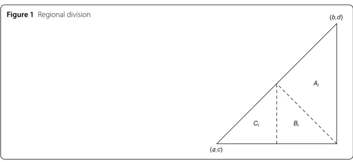
Figure 1Regional division
Step 5: IfBE>δ(δ is a given small number that is preassigned as the boundary error limit), then the calculation is continued toStep 6. Otherwise, the calculation is stopped, and one obtains the segmented approximate solution as follows:
H(x,y) =
⎧ ⎪ ⎪ ⎨ ⎪ ⎪ ⎩
HAj(x,y), (x,y)∈Aj,j= 0, 1, 2, . . . ,i; HBj(x,y), (x,y)∈Bj,j= 0, 1, 2, . . . ,i; HCi(x,y), (x,y)∈Ci.
(8)
Step 6: Settingi=i+ 1 andHAi(x,y) =HCi–1(x,y). Then, using the linesy=y0+ (y¯–y0)/(x¯– x1)(x–x1) andx=x¯, the areaCi–1is divided into three partsAi,Bi, andCi(see Fig.1):
Ai:x¯≤x≤x1,l1(x)≤y≤l2(x);
Bi:x¯≤x≤x1,y0≤y≤l1(x);
Ci:x0≤x≤ ¯x,y0≤y≤l2(x).
(9)
Step 7: Eq. (1) with the boundary conditionsh(x,y0) =f3(x),h(x,l1(x)) =HAi(x,l1(x)) is
solved by the Adomian decomposition method. In this process, the inverse operator L–1B is taken as follows:
L–1B =
y
y0 y
y0
dy dy– y–y0
l1(x) –y0
l1(x)
y0 y
y0
dy dy, (10)
whereHBi(x,y) ((x,y)∈Bi) denotes the solution obtained in this step. Step 8: Setx1=x¯,y1=y¯,f1(y) =HBi(x1,y), then proceed toStep 2.
3 The convergence theorem of the algorithm
Definition The norm of a continuous functionf(x) on the closed interval [a,b] is defined as follows:
f(x)[a,b]=max
x∈[a,b]
The norm of a continuous functionf(x,y) on the plane closed regionDis defined as fol-lows:
f(x,y)D= max
(x,y)∈Df(x,y). (12)
There relations (11) and (12) are considered theL∞-error. Thus, the approximate degree of congruence off(x,y) withg(x,y) onDshould be characterized byf(x,y) –g(x,y)D.
Theorem For an arbitrary small real numberδ> 0,there exists a natural number N> 0
such that when i>N(i is the number of iterations of the algorithm,namely the number of times dividing the area(2)),one has
BE=HCi(x,y0) –f3(x)
2
2<δ, (13)
if there exists a real number> 0such thatH(x,y) –h(x,y)D<,namely the approximate
solution H(x,y) ((x,y)∈D)uniformly converges to the exact solution h(x,y)of boundary problem(1)–(18).
Proof According to the continuity of the functionsHCi(x,y0) andf3(x) on [x0,x¯], one has
BE =
x¯
x0
HCi(x,y0) –f3(x) 2
dx
≤HCi(x,y0) –f3(x)
2
[x0,¯x]·(x¯–x0)
≤HCi(x,y0)[x0,x¯]+f3(x)[x0,x¯] 2
·b–a 2i
≤HCi(x,y)Ci+f3(x)[x0,x¯] 2
·b–a 2i
≤HCi(x,y) –h(x,y)Ci+h(x,y)Ci+f3(x)[x0,x¯] 2
·b–a 2i
≤HD(x,y) –h(x,y)D+h(x,y)D+f3(x)[a,b]
2 ·b–a
2i ≤M·2–i,
whereM= (+h(x,y)D+f3(x)[a,b])2·(b–a).
Thus, for an arbitrarily small real numberδ> 0, whileN= [log2(M/δ)] andi>N, the
resultBE<δis established.
Because we are unable to calculateH(x,y) –h(x,y)D, we define the residual error func-tion to characterize the accuracy of the approximate solufunc-tions. Define an error funcfunc-tion as follows:
Error(h) = Lxh+ Lyh+h+g(x,y). (14)
Then EE=Error(h(x,y))2
2 characterizes the accuracy of the approximate solutions to
Eq. (1), where · 2 denotes theL2-norm. IfEEandBE are equal to zero at the same
approximate solution, where the values ofEE,BEcharacterize the equation and boundary errors.
4 Application of this algorithm
4.1 The model for the effect of regional recharge of the triangle groundwater flow region
Syafrin and Serrano [24] used the model for the effect of regional recharge to study the groundwater flow in the Louisville aquifer. Serrano [25] studied a simple approach to groundwater modeling with decomposition. Dehghan [26] uses the orthogonal decom-position discrete empirical interpolation method (POD-DEIM) to prevent groundwater pollution. In this section, we reconsider the model for the effect of regional recharge on the triangle groundwater flow region. The governing equation of the model is as follows:
∂2h
∂x2 +
∂2h
∂y2 = –
Rg
T , 0≤x≤600, 0≤y≤x, (15)
with the boundary conditions
h(600,y) = – y
2
450,000+ 3y
1000+ 102, (16)
h(x,y) = – x
2
125,000+ 49x
5000+ 100, ony=x, (17)
h(x, 0) = – 3x
2
500,000+ 13x
1875+ 100, (18)
wherehis the hydraulic head [L];Rg is mean monthly recharge from rainfall [LT–1];T is the mean aquifer transmissivity [L2T–1]; and aand b are the aquifer horizontal
di-mensions in thexandydirection, respectively [L]. A typical recharge rate from rainfall
Rg= 10 mm/month, aquifer transmissivity ofT= 100 m2/month. Then Eq. (15) is rewrit-ten
Lxh(x,y) + Lyh(x,y) = –Rg
T. (19)
The specific process of the algorithm for the model is as follows:
Step 1: Seti= 0,x0= 0,y0= 0,x1= 600,y1= 600,l1(x) = –x+ 600,l2(x) =x, andC0= {(x,y)|0≤x≤600, 0≤y≤x}.
Step 2: Problem (15) with boundary conditions (16) and (17) is considered. Applying the inverse operator L–1C on the both sides of Eq. (15), we obtain
∞
n=0
hn=f2(y) +
x–y
600 –y
f1(y) –f2(y)
– L–1C Rg
T – L
–1
CLy ∞
n=0
hn, (20)
where
L–1C =
x
y
x
y
dx dx– x–y 600 –y
600
y
x
y
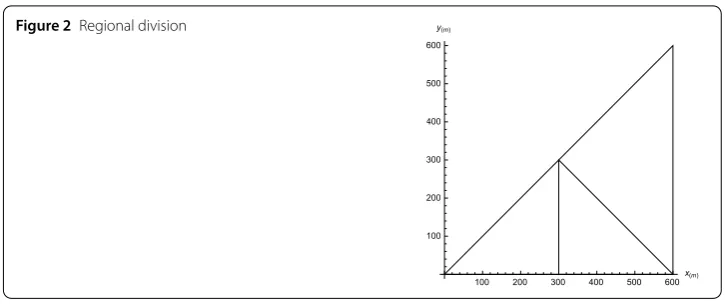
Figure 2Regional division
The following recursion formulae are constructed from the above equation:
h0=f2(y) +
x–y
600 –y
f1(y) –f2(y)
– L–1C Rg
T ,
hn= –L–1CLyhn–1, n= 1, 2, . . . .
(21)
From the recursion formulae (21), we obtainh0,h1, thenhn= 0 (n≥2), i.e., the solution
HC0 of (15) with conditions (16) and (17) is obtained as follows:
HC0(x,y) = –
43x2
900,000+ 21xy
500,000+ 4x
125–
y2
450,000– 111y
5000+ 100, (x,y)∈C0. (22)
Step 3: BecauseBE= 4524, we setHA1(x,y) =HC0(x,y) and continue to the next step. Step 4: Applying the linesx= 300 andy= 600 –x, the domainC0: 0≤x≤600, 0≤y≤x
is divided into three parts (see Fig.2):
A1: 300≤x≤600, 600 –x≤y≤x;
B1: 300≤x≤600, 0≤y≤600 –x;
C1: 0≤x≤300, 0≤y≤x.
(23)
Step 5: Solving the problem in the domainB1 with the boundary conditionsh(x, 0) =
f3(x),h(x, 600 –x) =HA1(x, 600 –x). After applying L
–1
B on the both sides of Eq. (15), the following recursion formulae are constructed:
h0=f3(x) +
y
600 –x
HA1(x, 600 –x) –f3(x)
– L–1B Rg
T, hn= –L–1B Lxhn–1, n= 1, 2, . . . ,
(24)
where
L–1B =
y
0
y
0
dy dy– y 600 –x
600–x
0
y
0
dy dy.
From the recurrence formulae, we obtainhn= 0 (n≥2), i.e., the solution is as follows:
HB1(x,y) = –
3x2
500,000+ 21xy
500,000+ 13x
1875– 11y2
250,000+ 43y
Step 6: Solving the problem onC1with the boundary conditionsh(y,y) =f2(y),h(300,y) =
HB1(300,y). After applying L–1C on both sides of Eq. (15), the following recursion formulae are constructed:
Thus, the solution is obtained as follows:
HC1= –
At this moment, the boundary errorBE= 0, so the calculation is stopped. The segment solution is obtained as follows:
H(x,y) =
4.2 A heterogeneous aquifer model of the triangular groundwater flow region
The governing differential equation of the model is as follows:
∂
Boundary conditions (16)–(18) are also considered in this model. Thus Eq. (28) is rewritten as follows:
Lxh(x,y) + Lyh(x,y) = –
The function 1/T(x,y) is expanded at the origin according to Taylor’s formula as follows:
where
The concrete process of the calculation for the model by the algorithm is as follows:
Step 1: Settingi= 0,x0= 0,y0= 0,x1= 600,y1= 600 andAi=∅,Bi=∅,Ci={(x,y)|0≤
x≤600, 0≤y≤x}.
Step 2: Settingx¯=x1/2,l1(x) =x1–x,l2(x) =x,˜l1(y) =x1–y,˜l2(y) =y.
Step 3: Problem (28) with the boundary conditionsh(x1,y) =f1(y) andh(y,y) =f2(y) is
considered by the ADM. Applying L–1
C on the both sides of Eq. (28), we obtain
From the aforementioned equation, the following recursion formulae are obtained:
h0=f2(y) +
Thus, then-term approximate Adomian solution of the problem onCiis obtained as fol-lows:
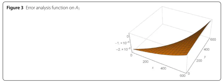
Figure 3Error analysis function onA1
Step 4: IfBE>δ(for example,δ= 0.001), seti=i+ 1,HAi(x,y) =HCi–1(x,y) and continue
to the next step. Otherwise, the calculation is stopped, as one obtains the segmented ap-proximate solution (8).
For the 3-term approximate solutionHC0,BE= 8.11375 < 0.01, so seti=i+ 1,HA1(x,y) = HC0(x,y) and continue to the next step.
Step 5: Using the linesx=x¯andy=x1–x, the domainCi–1is divided into three parts
(see Fig.2):
Ai:x¯≤x≤x1,l1(x)≤y≤l2(x);
Bi:x¯≤x≤x1,y0≤y≤l1(x);
Ci:x0≤x≤ ¯x,y0≤y≤l2(x).
(36)
Step 6: Solving the problem inBiwith the boundary conditionsh(x, 0) =f3(x),h(x,x1–
x) =HAi(x,x1–x). After applying L–1B on both sides of Eq. (28), the following recursion formulae are constructed:
h0=f3(x) +
y x1–x
h(x,x1–x) –f3(x)
– L–1B Rgt1,
hn= –L–1B Lxhn–1– L–1B Rgtn+1– L–1B
∂T
∂x
n–1
j=0
tn–j
∂hj
∂x +
∂T
∂y
n–1
j=0
tn–j
∂hj
∂y
,
n= 1, 2, . . . ,
where
L–1B =
y
0
y
0
dy dy– y
x1–x
x1–x
0
y
0
dy dy.
From the above recurrence formulae, then-term approximate Adomian solution of the problem onBiis obtained as follows:
HBi(x,y) =
n
i=0
hi. (37)
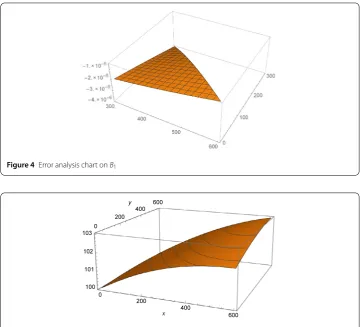
For the 3-term approximate solutionHB1(x,y),EE= 2.23031×10
–7, and the graph of
Figure 4Error analysis chart onB1
Figure 5The segmented solutionH(x,y), where (x,y)∈D
Step 7: Setx1=x¯,y1=y1/2,f1(y) =HBi(x1,y), then go toStep 2.
In the same way, the calculation is repeated. Sincei= 2,BE= 0.007, the calculation is stopped, we obtain the segmented approximate solution (as shown in Fig.5) as follows:
H(x,y) =
⎧ ⎪ ⎪ ⎪ ⎪ ⎪ ⎪ ⎪ ⎪ ⎨ ⎪ ⎪ ⎪ ⎪ ⎪ ⎪ ⎪ ⎪ ⎩
HA1(x,y), (x,y)∈A1; HB1(x,y), (x,y)∈B1; HA2(x,y), (x,y)∈A2; HB2(x,y), (x,y)∈B2;
HC2(x,y), (x,y)∈C2.
(38)
5 Discussion and conclusions
Through the proposed algorithm, we can make the boundary error of the BVP smaller than any positive number. As for the model for the effect of regional recharge on the plane trian-gle groundwater flow region, we have obtained the segmented exact solution of the prob-lem by our new algorithm, which satisfies the governing equation and all of the boundary conditions of the boundary value problem.
results are compared with the results in [23], the boundary has been controlled to smaller than any real number, but not in [23]. From those processes, we can validate the effective-ness of the algorithm.
If the remainder operator R in Eq. (1) were to include a nonlinear operator, then our proposed algorithm would become an algorithm for solving of a second-order nonlinear partial differential equation on a triangle domain. Thus the proposed method can be used to solve either a general second-order nonlinear or a linear partial differential equation on a plane triangle domain.
We will consider modifying the ADM with supplemental algorithms depending on whether it is an IVP, or various types of BVPs, e.g., whether it is a Dirichlet BVP, Neu-mann BVP, Robin BVP, or possible combinations of mixed boundary conditions. Further-more, we will always need to consider modifying the ADM with supplemental algorithms depending on the shape of the boundary contours, i.e., rectangular boundary contours are usually simpler; for highly irregular boundary contours, we can do so because of the versatility of the ADM.
In addition, based on the idea of the algorithm, other methods (such as homotopy per-turbation method, the variational iteration method, the homotopy analysis method [6,
11–13,27,28], and the segmented technique are used to solve the boundary value prob-lem of a second-order partial differential equation on a plane triangle area. Now, we take the homotopy perturbation method as an example to consider the model for the effect of regional recharge of the triangle groundwater flow region. Specific steps are as follows.
Step 1: Problem (15) with boundary conditions (16) and (17) is considered. First, the homotopy equations of Eq. (15) are constructed as follows:
Lxh(x,y) +pLyh(x,y) = –
Rg
T. (39)
Then, substitutingh(x,y) =∞i=0piu
i(x,y) into (39), then letting the coefficients of vari-ous powers ofpbe zero, we obtain a series of systems foruias follows:
Lxu0(x,y) +
1
10,000= 0, (40)
Lyui–1(x,y) + Lxui(x,y) = 0, i= 1, 2, . . . . (41)
Solving this system, we obtainedhn= 0 (n≥2), and the solutionHA1(x,y) of (15) with
conditions (16) and (17) is obtained again as follows:
HA1(x,y) = –
43x2
900,000+ 21xy
500,000+ 4x
125–
y2
450,000– 111y
5000 + 100, (x,y)∈C0. (42)
Step 2: Solving the problem in the domainB1in Fig.2with the boundary conditions
h(x, 0) =f3(x),h(x, 600 –x) =HA1(x, 600 –x). There the homotopy equations of Eq. (15) are
constructed as follows:
pLxh(x,y) + Lyh(x,y) = –Rg
T. (43)
hn= 0 (n≥2), and the solutionHB1(x,y) of (15) with conditions (16) and (17) is obtained
again.
Step 3: Solving the problem onC1in Fig.2with the boundary conditionsh(y,y) =f2(y),
h(300,y) =HB1(300,y).There the homotopy equations of Eq. (15) are constructed as
fol-lows:
Lxh(x,y) +pLyh(x,y) = –
Rg
T. (44)
Then, substitutingh(x,y) =∞i=0piui(x,y) into (44), then letting the coefficients of various powers ofpbe zero, we obtain a series of systems forui. Solving this system, we obtained
hn= 0 (n≥2), and the solutionHC1(x,y) of (15) with conditions (16) and (17) is obtained
again. Thus, the segment solution (26) is obtained again. The result shows the effectiveness of the idea of the algorithm.
Acknowledgements
Grateful acknowledgement is made to Mr. Yinshan who gave me considerable help by means of suggestion and criticism. His encouragement and unwavering support has sustained me through frustration and depression. Without his pushing me ahead, the completion of this thesis would be impossible. In addition, I deeply appreciate the contribution to this thesis made in various ways by Mr. Chaolu and Rach.
Funding
The present work was supported by the National Natural Science Foundation of China (No. 11571008, 11661059), Natural Science Foundation of Inner Mongolia (No. 2016MS0109), Research Projects of Higher Education of Inner Mongolia (NJZY094), Key Projects of Inner Mongolia University of Technology (ZD201515).
Competing interests
As far as we know, there are no conflicts of interest, financial or other conflicts between the designated author and the editors, reviewers, and readers of this magazine.
Authors’ contributions
The author YY’s contribution is to discover the subject matter, complete the calculation, and derivation process with YW, CT’s contribution to this article is to help with machine calculation, and RR’s contribution is to correct the errors in the literature. All authors read and approved the final manuscript.
Author details
1College of Sciences, Inner Mongolia University of Technology, Hohhot, China.2College of Information Engineering, Shanghai Maritime University, Shanghai, China.3College of Sciences and Arts, Shanghai Maritime University, Shanghai, China.4Hartford, USA.
Publisher’s Note
Springer Nature remains neutral with regard to jurisdictional claims in published maps and institutional affiliations.
Received: 27 April 2019 Accepted: 4 September 2019
References
1. Bluman, G.W., Kumei, S.: Symmetries and Differential Equations. Springer, New York (1989) 2. Olver, P.J.: Applications of Lie Groups to Differential Equations. Springer, New York (1999)
3. He, J.H.: A coupling method of a homotopy technique and a perturbation technique for non-linear problems. Int. J. Non-Linear Mech.35, 37–43 (2000)
4. He, J.H.: An elementary introduction to the homotopy perturbation method. Comput. Math. Appl.57, 410–412 (2009)
5. Liao, S.J.: The proposed homotopy analysis technique for the solution of nonlinear problems. PhD thesis, Shanghai Jiao Tong University (1992)
6. Dehghan, M., Manafian, J., Saadatmandi, A.: Solving nonlinear fractional partial differential equations using the homotopy analysis method. Numer. Methods Partial Differ. Equ.26, 448–479 (2010)
7. Adomian, G.: A review of the decomposition method in applied mathematics. J. Math. Anal. Appl.135, 501–544 (1988)
8. Rach, R.: A new definition of the Adomian polynomials. Kybernetes37, 910–955 (2008)
9. Fan, E.G.: Extended tanh-function method and its applications to nonlinear equations. Phys. Lett. A277, 212–218 (2000)
11. Tatari, M., Dehghan, M.: On the convergence of He’s variational iteration method. J. Comput. Appl. Math.207, 121–128 (2007)
12. Anjum, N., He, J.H.: Laplace transform: making the variational iteration method easier. Appl. Math. Lett.92, 134–138 (2019)
13. Dehghan, M., Aryanmehr, S., Eslahchi, M.R.: A technique for the numerical solution of initial-value problems based on a class of Birkhoff-type interpolation method. J. Comput. Appl. Math.244, 125–139 (2013)
14. Adomian, G., Rach, R.: Analytic solution of nonlinear boundary-value problems in several dimensions by decomposition. J. Math. Anal. Appl.174, 118–137 (1993)
15. Wazwaz, A.M.: A note on using Adomian decomposition method for solving boundary value problems. Found. Phys. Lett.13, 493–498 (2000)
16. Wazwaz, A.M.: The numerical solution of sixth-order boundary value problems by the modified decomposition method. Appl. Math. Comput.118, 311–325 (2001)
17. Dehghan, M., Salehi, R.: Solution of a nonlinear time-delay model in biology via semi-analytical approaches. Comput. Phys. Commun.181, 1255–1265 (2010)
18. Dehghan, M., Tatari, M.: Finding approximate solutions for a class of third-order non-linear boundary value problems via the decomposition method of Adomian. Int. J. Comput. Math.87, 1256–1263 (2010)
19. Duan, J.S., Rach, R., Wazwaz, A.M.: Steady-state concentrations of carbon dioxide absorbed into phenyl glycidyl ether solutions by the Adomian decomposition method. J. Math. Chem.53, 1054–1067 (2015)
20. Adomian, G.: Stochastic Systems. Academic Press, New York (2013)
21. Shidfar, A., Garshasbi, M.: A weighted algorithm based on Adomian decomposition method for solving an special class of evolution equations. Commun. Nonlinear Sci. Numer. Simul.14, 1146–1151 (2009)
22. Yun, Y.S., Chaolu, T., Duan, J.S.: A segmented and weighted Adomian decomposition algorithm for boundary value problem of nonlinear groundwater equation. Math. Methods Appl. Sci.37, 2406–2418 (2014)
23. Wen, Y., Yun, Y.S.: Segmented Adomian approximate solution of heterogeneous aquifer model of ground-water flow. Adv. Appl. Math.37, 435–441 (2017)
24. Syafrin, T., Serrano, S.E.: Regional groundwater flow in the louisville aquifer. Ground Water53, 550–557 (2015) 25. Serrano, S.E.: A simple approach to groundwater modelling with decomposition. Hydrol. Sci. J.58, 177–185 (2013) 26. Dehghan, M., Abbaszadeh, M.: A combination of proper orthogonal decomposition discrete empirical interpolation
method (POD-DEIM) and meshless local RBF-DQ approach for prevention of groundwater contamination. Comput. Math. Appl.75, 1390–1412 (2018)
27. He, J.H.: Homotopy perturbation method with an auxiliary term. Abstract and Applied Analysis (2012)