R E S E A R C H
Open Access
Iterative learning control for MIMO
second-order hyperbolic distributed
parameter systems with uncertainties
Xisheng Dai
1*, Chao Xu
2, Senping Tian
3and Zhenglin Li
1*Correspondence:
1School of Electrical and
Information Engineering, Guangxi University of Science and Technology, Liuzhou, 545006, China Full list of author information is available at the end of the article
Abstract
In this paper, we consider an iterative learning control (ILC) problem for a class of multiinput-multioutput (MIMO) second-order hyperbolic distributed parameter systems with uncertainties. A P-type ILC scheme is proposed in the iteration
procedure for distributed systems with an initial deviation in the state. A convergence of tracking error with respect to the iteration index can be guaranteed in the sense of L2norm. Feasibility in theory of the iterative learning algorithm with difference method is proposed. Numerical simulation results are presented to illustrate the effectiveness of the proposed ILC approach.
Keywords: iterative learning control; second-order hyperbolic distributed parameter systems; convergence
1 Introduction
ILC is an intelligent control methodology for repetitive processes and tasks over a finite interval. ILC was first formulated mathematically by Arimotoet al.[]. In the last three decades, it has been constantly studied and widely applied in various engineering prac-tice, such as robotics, freeway traffic control, biomedical engineering, industrial process control,et cetera[–]. The major benefit of ILC are completely tracking feasible refer-ence trajectories (or evolutional profiles) for that complex systems include uncertainty or nonlinear. It can be achieved only based on the input and output signals [–]. It is a truly model-free method motivated by the human trial-and-error experience in prac-tice.
Despite ILC has been widely investigated for finite-dimensional systems, research work of related to spatial temporal processes are quiet few and even less using infinite-dimensional framework. Qu [] proposed an iterative learning algorithm for boundary control of a stretched moving string, which is a pioneer work of extending the ILC frame-work to distributed parameter systems. Tension control system is studied in [] by using the PD-type learning algorithm. Both P-type and D-type iterative learning algorithms based on the operator semigroup theory are designed for one-dimensional distributed parameter systems governed by parabolic PDEs in [] and have been extended to a class of impulsive first-order distributed parameter systems in []. In [], a steady state ILC scheme is proposed for single-input-single-output nonlinear PDEs. A D-type
tory ILC scheme is applied to the boundary control of a class of inhomogeneous heat equations in [], where the heat flux at one side is the control input, whereas the tem-perature measurement at the other side is the control output. The learning convergence of ILC is guaranteed by transforming the inhomogeneous heat equation into its integral form and exploiting the properties of the embedded Jacobi theta functions. In [], for applied convenience, using Crank-Nicholson discretization, ILC for a heat equation is de-signed, where the control allows the selection of a finite number of points for sensing and actuation. Recently, a frequency domain design and analysis framework of ILC for inho-mogeneous distributed parameter systems are proposed in []. However, these works did not involve MIMO second-order hyperbolic distributed parameter systems.
The control problem of hyperbolic distributed parameter systems has been frequently encountered in many dynamic processes, for example, wave transportation, fluid dynam-ics, elastic vibration. In [], a P-type ILC algorithm is proposed for a first-order hyper-bolic distributed parameter system arising in a nonisothermal tubular reactor using a set of ordinary differential equations (ODEs) for model approximation. In addition, ILC prob-lem is considered in [] for a first-order strict hyperbolic distributed parameter system in a Hilbert space, where convergence conditions are given based on P-type algorithms and require the initial state value to be identical.
In this paper, an ILC problem is considered for a class of MIMO second-order hyper-bolic distributed parameter systems with uncertainties. A P-type ILC scheme is intro-duced, and a sufficient condition for tracking error convergence in the sense of Lnorm
is given. The conditions do not require analytical solutions but only bounds and an ap-propriate norm space assumption for uncertainties of the system coefficients matrix. The proposed control scheme is the first work on extension to MIMO second-order hyperbolic distributed parameter systems with admissible initial state error. On the other hand, the convergence analysis is more complex than for finite-dimensional systems because it in-volves time, space, and the iterative domain. We do not simplify the infinite-dimensional systems to finite-dimensional systems or replace them with discrete-time equivalences (see []). Only in simulation, in order to illustrate the effectiveness of the presented ILC approach, we used the forward difference method to discretize the infinite-dimensional systems.
Notation The superscript ‘T’ denotes the matrix transposition;Iand denote the iden-tity matrix and zero matrix of appropriate dimensions, respectively. For ann-dimensional
constant vector q = (q,q, . . . ,qn)T, its Euclid norm is defined as q=
n
i=qi. The
spectrum norm of an n×n-order square matrix A is defined as A=λmax(ATA),
whereλmax(·) (λmin(·)) represents the maximum (minimum) eigenvalue. Let L() be the
set of measurable functionsqdefined on a bounded domain∈Rm such thatq
L =
|q(x)|dx<∞. Ifqi(x)∈L() (i= , , . . . ,k) (for convenience, we denote L() as
L(; R)), then we write q(x) = (q
(x), . . . ,qn(x))∈Rn∩L(), andqL=
qT(x)q(x) dx.
For w(x,t) :×[,T]→Rmsuch that w(·,t)∈Rm∩L(),t∈[,T], givenλ> , its (L;λ)
norm is defined as
w(L;λ)= sup
≤t≤T
w(·,t)L()e–λt
2 ILC system description
We consider the following MIMO second-order hyperbolic distributed parameter system governed by partial differential equations:
∂q(x,t)
∂t =Dq(x,t) –A(t)
∂q(x,t)
∂t +B(t)u(x,t),
y(x,t) =C(t)q(x,t) +G(t)u(x,t), ()
where (x,t)∈×[,T], that is,x,tdenote the space and time variables, respectively, T is given, is a bounded open subset of Rm with smooth boundary∂, q(·,·)∈Rn,
u(·,·)∈Ru, and y(·,·)∈Ry are the state vector, input vector, and output vector of the
systems, respectively, D is a bounded positive constant diagonal matrix, that is, D=
diag{d,d, . . . ,dn}, <pi≤di<∞(i= , , . . . ,n), andpiare known,=
m
i=
∂ ∂xi is the
Laplacian operator defined over,A(t) is a bounded and positive definite matrix for all t∈[,T], andB(t), C(t), andG(t) are the bounded time-varying uncertain matrices of appropriate dimensions.
The initial and boundary conditions of () are given as
q(x,t) = , (x,t)∈∂×[,T], ()
q(x, ) =ϕ(x), ∂q(x,t)
∂t
t=
=ψ(x). ()
The control target is to determine an input vector ud(x,t) such that the output vector y(x,t)
is capable tracking a desired feasible trajectory yd(x,t), namely seeking a corresponding
desired input ud(x,t) such that the actual output of the system (),
y∗(x,t) =C(t)qd(x,t) +G(t)ud(x,t),
approximates the desired output yd(x,t). Because in the system there exists uncertainty,
it is difficult to obtain a complete tracking, so we will gradually gain the control sequence
uk(x,t), using the ILC method, such that
lim
k→∞uk(x,t) = ud(x,t),
where thekth iteration control input satisfies
∂qk(x,t)
∂t =Dqk(x,t) –A(t)∂qk∂(tx,t)+B(t)uk(x,t),
yk(x,t) =C(t)qk(x,t) +G(t)uk(x,t).
()
Assumption . We assume that there exists a unique bounded classic solution q(x,t) for system (). Thus, for a desired output yd(x,t), there exists a unique ud(x,t) such that
∂qd(x,t)
∂t =Dqd(x,t) –A(t)∂qd∂(tx,t)+B(t)ud(x,t),
yd(x,t) =C(t)qd(x,t) +G(t)ud(x,t),
()
satisfying the initial and boundary conditions
qd(x, ) = qd(x),
∂qd(x,t) ∂t
t=
=q˙d(x), x∈, ()
where qd(x,t) is the desired state, and (qd(x),q˙d(x)) is the initial value of the desired state.
Assumption . In a learning process, we assume the following boundary and initial con-ditions:
qk(x,t) = , (x,t)∈∂×[,T], ()
qk(x, ) =ϕk(x),
∂qk(x, )
∂t =ψk(x), x∈. ()
The functionsϕk(x),ψk(x) satisfy
∂ϕk+
∂x –
∂ϕk(x) ∂x
L()≤
lαk, ψk+–ψkL()≤lβk, ()
wherel,lare constants, andα,β∈[, ).
Remark . Assumption . is a necessary condition for ILC method. Assumption . means that, in the initial state, there may exist an error and the identical initial condition in ILC systems () is not required. On the other hand, from practical point of view, in iterations, the initial condition reset should be closer and closer to the initial value of the desired state, so condition () is reasonable.
3 ILC design and convergence analysis
In this paper, we employ the following P-type ILC law:
uk+(x,t) = uk(x,t) + (t)ek(x,t), ()
where (t) is the learning gain. For a brief presentation, let
ek+(x,t) = yd(x,t) – yk+(x,t),
¯
qk(x,t) = qk+(x,t) – qk(x,t),
¯
uk(x,t) = uk+(x,t) – uk(x,t),
where ek+(x,t) is the tracking error of the (k+ )th iteration. Then the control target can
be rewritten as
lim
k→∞
ek(·,t)L()= , ∀t∈[,T]. ()
We need the following technical lemmas, which are widely used in the proof of the main theorem.
Lemma .([]) Let A∈Rn×m,B∈Rn×l,ζ∈Rm,η∈Rl.Then we have
ζTATBη≤
ζTATAζ+ηTBTBη. ()
Lemma .([]) Let a nonnegative real series{ak}∞k=satisfy
ak+≤rak+zk, ()
where≤r< andlimk→∞zk= .Then we have
lim
k→∞ak= . ()
Theorem . Consider the ILC updating law()applied to the repetitive system()under (), ()and satisfying Assumptions.and..If the gain matrix (t)satisfies
I–G(t) (t)≤ρ∈[, ), ρ< , ()
then the tracking error converges to zero in the sense ofLnorm for all t∈[,T]as k→ ∞,
that is,
lim
k→∞
ek(·,t)L()= , ∀t∈[,T]. ()
Proof According to the learning law (), we have
ek+(x,t) = ek(x,t) – yk+(x,t) + yk(x,t)
= ek(x,t) –G(t)
uk+(x,t) – uk(x,t)
–C(t)qk+(x,t) – qk(x,t)
=I–G(t) (t)ek(x,t) +C(t)
qk+(x,t) – qk(x,t)
eˆk(x,t) +qˆk(x,t), ()
where
ˆ
ek(x,t)
I–G(t) (t)ek(x,t), qˆk(x,t)C(t)
qk+(x,t) – qk(x,t)
.
Then, by Lemma . we have
eTk+(x,t)ek+(x,t) =
ˆ
eTk(x,t) +qˆTk(x,t)eˆk(x,t) +qˆk(x,t)
≤eˆTk(x,t)ˆek(x,t) +qˆTk(x,t)ˆqk(x,t)
≤λG eTk(x,t)ek(x,t) + λCq¯Tk(x,t)¯qk(x,t), ()
where
λG = max
≤t≤T
I–G(t) (t)
, λC= max
≤t≤T
C(t)
Meanwhile, because
By the Bellman-Gronwall inequality we have
Choosing a sufficiently large constantλ> and multiplying both sides of () bye–λt, we
On the other hand, according to the P-type ILC law (), we have
uk+(·,t) –uk(·,t)
Then, by (), we can select a suitable largeλsuch that
we have the convergence
lim
k→∞
ek(·,t)L()= , t∈[,T]. ()
This completes the proof of Theorem ..
Remark . In Theorem ., we must point out that () requiresG(t) to be a nonsingular matrix (or regular matrix), that is, there exists a direct channel in between the output and input for systems (). We will consider the caseG(t) = in the future.
4 Numerical simulations
In order to illustrate the effectiveness of the proposed ILC scheme, we give the following specific numerical example:
and (x,t)∈[, ]×[, ]. The desired evolutionary profile vector is given as the iterative learning:
the input value of the controlling at the beginning of learning are set to be andα=β= in (). Then the condition of Theorem . is satisfied. that is,I–G = . < .. We use the following forward difference method:
∂qk(x,t)
whereh,τ are space and time sizes, respectively, and (xi,tj) is discrete point.
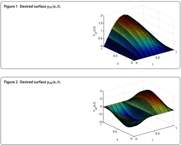
Figure 1 Desired surfaceyd1(x,t).
Figure 2 Desired surfaceyd2(x,t).
• Step. Iterative numberk= (for convenience, the iterative time begins from ). .. Let control inputu(x,t) = withq(,t) = = q(,t),q(x, ),∂q∂(tx,),A(t),
B(t),D. Based on the second-order differential equations and above difference method, we can solve () and obtainq(x,t).
.. By the output equationy(x,t) =C(t)q(x,t) +G(t)u(x,t)we calculatey(x,t).
.. Calculatee(x,t) = yd(x,t) – y(x,t).
• Step. Iterative numberk= ,u(x,t) = u(x,t) + (t)e(x,t).
• Step. Repeating Step , but with control inputu(x,t)(= ), we obtaine(x,t).
• Step. At thekth iteration, if the tracking errorek(x,t)is less than the given error, then end, else continue.
It should be pointed out that we did not need know (but require to be bounded) the uncertain coefficientsA(t),B(t),C(t),G(t) in practical process control; we only need re-member the tracking error and calculate (offline) the next time control input uk+(x,t).
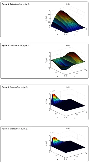
The simulation results obtained using this iterative learning algorithm and difference method are shown in Figures -.
Figures and show the desired profile, Figures and show the relative profile at the twentieth iteration, Figures and show the error curved surface, whereeki(x,t) =
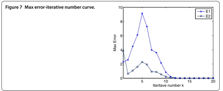
ydi(x,t) –yki(x,t),i= , ,k= . Figure is the curve chart describing the variation of the
maximum tracking error with iteration numbers. Numerically, in the twentieth iteration, the absolute values of the maximum tracking error are .×– and .×–. These simulation results demonstrate the efficacy of the ILC law ().
5 Conclusions
Figure 3 Output surfaceyk1(x,t).
Figure 4 Output surfaceyk2(x,t).
Figure 5 Error surfaceek1(x,t).
Figure 7 Max error-iterative number curve.
that guarantee the tracking error convergence in the sense of Lnorm. A simulation
ex-ample is given to illustrate the effectiveness of the proposed algorithm.
Competing interests
The authors declare that they have no competing interests.
Authors’ contributions
This work was carried out in collaboration between all authors. XD raised these interesting problems in this research. CX, ST, and XD proved the theorems, interpreted the results, and wrote the article. The numerical example is given by ZL. All authors defined the research theme, read, and approved the manuscript.
Author details
1School of Electrical and Information Engineering, Guangxi University of Science and Technology, Liuzhou, 545006, China. 2The State Key Laboratory of Industrial Control Technology, Institute of Cyber-Systems and Control, Zhejiang University,
Hangzhou, Zhejiang 310027, China.3School of Automation Science and Engineering, South China University of
Technology, Guangzhou, 510640, China.
Acknowledgements
The authors are grateful to the referees for their careful reading of the manuscript and valuable comments. The authors thank for the help from the editor too. The work was supported by the National Natural Science Foundation of China (Nos. 61364006, 61374104) and Key Laboratory of Intelligent integrated automation of Department of Guangxi Education, Project of Outstanding Young Teachers’ Training in Higher Education Institutions of Guangxi.
Received: 29 January 2016 Accepted: 30 March 2016
References
1. Arimoto, S, Kawamura, S, Miyazaki, F: Bettering operation of robots by learning. J. Robot. Syst.1(2), 123-140 (1984) 2. Oh, S, Bien, Z, Suh, I: An iterative learning control method with application for the robot manipulator. IEEE J. Robot.
Autom.4(5), 508-514 (1988)
3. Hou, ZS, Xu, JX, Freeway, ZHW: Traffic control using iterative learning control based ramp metering and speed signaling. IEEE Trans. Veh. Technol.56(2), 466-477 (2007)
4. Wang, YQ, Dassau, E, Doyle, FJ III: Close-loop control of artificial pancreaticβ-cell in type diabetes mellitus using model predictive iterative learning control. IEEE Trans. Biomed. Eng.57(2), 211-219 (2010)
5. Ruan, XE, Wan, BW: The iterative learning control for saturated nonlinear industrial control systems with delay. Acta Autom. Sin.27(2), 219-223 (2001)
6. Chen, HF: Almost sure convergence of iterative learning control for stochastic systems. Sci. China, Ser. F, Inf. Sci.46(1), 67-70 (2003)
7. Chen, WS, Zhang, ZQ: Nonlinear adaptive learning control for unknown time-varying parameters and unknown time-varying delays. Asian J. Control13(6), 903-913 (2011)
8. Liu, SD, Wang, JR, Wei, W: A study on iterative learning control for impulsive differential equations. Commun. Nonlinear Sci. Numer. Simul.24(1-3), 4-10 (2015)
9. Zhang, CL, Li, JM: Adaptive iterative learning control of non-uniform trajectory tracking for strict feedback nonlinear time-varying systems with unknown control direction. Appl. Math. Model.39(10-11), 2942-2950 (2015)
10. Moore, KL: Iterative Learning Control for Deterministic Systems. Springer, London (1993)
11. Bien, Z, Xu, JX: Iterative Learning Control-Analysis, Design, Integration and Applications. Kluwer Academic, Boston (1998)
12. Xu, JX, Tan, Y: Linear and Nonlinear Iterative Learning Control. Lecture Notes in Control and Information Science, vol. 291. Springer, Berlin (2003)
13. Chen, YQ, Wen, CY: Iterative Learning Control-Convergence, Robustness and Applications. Lecture Notes in Control and Information Sciences, vol. 248. Springer, Berlin (2003)
15. Qu, ZH: An iterative learning algorithm for boundary control of a stretched moving string. Automatica38(1), 821-827 (2002)
16. Zhao, H, Rahn, CD: Iterative learning velocity and tension control for single span axially moving materials. J. Dyn. Syst. Meas. Control130(5), 051003 (2008)
17. Xu, C, Arastoo, R, Schuster, E: On iterative learning control of parabolic distributed parameter systems. In: Proc. of 17th Mediterranean Conference on Control Automation, Makedonia Palace, Thessaloniki, Greece, pp. 510-515 (2009) 18. Yu, XL, Wang, JR: Uniform design and analysis of iterative learning control for a class of impulsive first-order
distributed parameter systems. Adv. Differ. Equ.2015, 261 (2015)
19. Huang, DQ, Xu, JX: Steady-state iterative learning control for a class of nonlinear PDE processes. J. Process Control
11(8), 1155-1163 (2011)
20. Huang, DQ, Xu, JX, Li, XF, Xu, C, Yu, M: D-type anticipator iterative learning control for a class in homogeneous heat equations. Automatica49(8), 2397-2408 (2013)
21. Cichy, B, Gakowski, K, Rogers, E: Iterative learning control for spatio-temporal dynamics using Crank-Nicholson discretization. Multidimens. Syst. Signal Process.23(1-2), 185-208 (2012)
22. Huang, DQ, Li, XF, Xu, JX, Xu, C, He, W: Iterative learning control of inhomogeneous distributed parameter systems -frequency domain design and analysis. Syst. Control Lett.72, 22-29 (2014)
23. Choi, JH, Seo, BJ, Lee, KS: Constrained digital regulation of hyperbolic PDE: a learning control approach. Korean J. Chem. Eng.18(5), 606-611 (2001)
24. Dai, XS, Tian, SP: Iterative learning control for first order strong hyperbolic distributed parameter systems. Control Theory Appl.29(8), 1086-1089 (2012)