R E S E A R C H
Open Access
A generalization of the Mittag–Leffler
function and solution of system of fractional
differential equations
Junsheng Duan
1**Correspondence:
1School of Sciences, Shanghai Institute of Technology, Shanghai, P.R. China
Abstract
The solutions of system of linear fractional differential equations of incommensurate orders are considered and analytic expressions for the solutions are given by using the Laplace transform and multi-variable Mittag–Leffler functions of matrix arguments. We verify the result with numeric solutions of an example. The results show that the Mittag–Leffler functions are important tools for analysis of a fractional system. The analytic solutions obtained are easy to program and are approximated by symbolic computation software such as MATHEMATICA.
Keywords: Fractional calculus; Fractional derivative; Mittag–Leffler function; Fractional differential equation
1 Introduction
Fractional calculus studies the several different possibilities of defining integral and deriva-tive of arbitrary order, generalizing the classical integration operatorJf(t) =0tf(τ)dτand differentiation operatorDf(t) =dtd f(t). In this regard, the common definitions include the Grünwald–Letnikov fractional integral and derivative, the Riemann–Liouville fractional integral and derivative, and the Caputo fractional derivative [1–9].
It is found that fractional calculus can describe memory phenomena and hereditary properties of various materials and processes [2–7,10]. In recent decades, fractional cal-culus has been applied to different fields of science and engineering, covering viscoelas-ticity theory, non-Newtonian flow, damping materials [4,7,11,12], anomalous diffusion [13–16], control and optimization theory [17–19], financial modeling [20,21], and so on. For the scalar functionf(t) ona<t< +∞, the Riemann–Liouville fractional integral of orderβis defined as
aJtβf(t) =
t a
(t–τ)β–1
(β) f(τ)dτ, (1)
forβ> 0, andf(t) forβ= 0. The Riemann–Liouville and Caputo fractional derivatives of orderαhave the forms
R aD
α
tf(t) =
dn dtn
aJtn–αf(t)
, 0 <n– 1 <α≤n, (2)
and
aDαtf(t) =aJtn–αf(n)(t), 0 <n– 1 <α≤n, (3)
respectively.
Fractional differential equations on scalar functions, including the existence, uniqueness and stability, and the analytic and numeric methods of solutions, were studied by many scholars [3–9,13,15,17,22–27]. In particular, new numerical schemes were designed [9,
23,24,28], and a Lie symmetry analysis was given and the conservation laws for fractional evolution equations were systematically investigated [29–32]. The solutions of many frac-tional differential equations involve a class of important special functions—Mittag–Leffler functions (AMS 2000 Mathematics Subject Classification 33E12). The Mittag–Leffler function with two parameters is defined by the series expansion [5,33]
Eλ,ρ(z) =
∞
k=0 zk
(λk+ρ), λ> 0,ρ> 0,z∈C, (4)
where (·) is Euler’s gamma function. The special case of λ=ρ= 1 degenerates to the exponential function, E1,1(z) =ez. We note that the Mittag–Leffler functions were also used to define new fractional derivatives [34,35].
The Laplace transform is an effective tool for the analysis of linear fractional differential equations. It is defined for a functionf(t) as
Lf(t)=f˜(s) = +∞
0
f(t)e–stdt, Re(s) >c. (5)
The Laplace transforms of the fractional integral and the Caputo fractional derivative are
L0Jtαf(t)=s–αf˜(s), α> 0, (6)
and
L0Dα
tf(t)
=sαf˜(s) –
n–1
k=0
sα–1–kf(k)0+, 0 <n– 1 <α≤n. (7)
Atanackovic and Stankovic [36] introduced the system of fractional differential equa-tions into the analysis of lateral motion of an elastic column fixed at one end and loaded at the other. Daftardar-Gejji and Babakhani [37] and Deng et al. [38] studied the existence, uniqueness and stability for solution of system of linear fractional differential equations with constant coefficients. Other references include [39–41]. In the above literature, solu-tions of the fractional differential system were given for the case of a commensurate order system.
In this paper, we focus on the system of linear fractional differential equations of in-commensurate orders and give analytic expressions for the solutions by using the Laplace transform and multi-variable Mittag–Leffler functions of matrix arguments. We verify the result with numeric solutions of an example.
In the sequel, we will use the Caputo fractional derivatives and denote0Dα
tf(t) byDαtf(t)
for short.
2 A generalization of the Mittag–Leffler function
We introduce ann-variable Mittag–Leffler function withn+ 1 parameters as
E(α1,α2,...,αn),β(t1,t2, . . . ,tn)
The explicit form of the first several terms on the right hand side is
1
The special case of the single variable, i.e.n= 1, degenerates to the Mittag–Leffler func-tion with two parameters as
E(α),β(t) =
The two-variable case, i.e.n= 2, is
E(α1,α2),β(t1,t2) =
large enoughk, we have
αj1+αj2+· · ·+αjk+β≥kα1+β> 2.
So it follows that
We estimate the general term of the series in Eq. (8) as
n
j1,j2,...,jk=1
tj1tj2. . .tjk (αj1+αj2+· · ·+αjk+β)
≤ 1
(kα1+β)
n
j1,j2,...,jk=1
|tj1tj2. . .tjk|
= 1
(kα1+β)
|t1|+|t2|+· · ·+|tn|
k
. (11)
It is well known that the dominant series
∞
k=0
1
(kα1+β)
|t1|+|t2|+· · ·+|tn|
k
converges to the Mittag–Leffler functionEα1,β(|t1|+|t2|+· · ·+|tn|).
If in the definition (8) the parameters satisfyα1=α2=· · ·=αn=α, then then-variable
Mittag–Leffler function in Eq. (8) also degenerates to the Mittag–Leffler function with two parameters as
E(α,α,...,α),β(t1,t2, . . . ,tn) =
1
(β)+
∞
k=1
1
(αk+β)
n
j1,j2,...,jk=1
tj1tj2. . .tjk
= 1
(β)+
∞
k=1
(t1+t2+· · ·+tn)k
(αk+β)
=Eα,β(t1+t2+· · ·+tn). (12)
In particular, ifα1=α2=· · ·=αn=β= 1, then-variable Mittag–Leffler function in Eq. (8)
degenerates to the exponential function
E(1,1,...,1),1(t1,t2, . . . ,tn) =E1,1(t1+t2+· · ·+tn) =et1+t2+···+tn. (13)
We remark that different versions of multi-variable Mittag–Leffler functions were pre-sented, such as in [43–46]. But they are not exactly the same as the version in this paper.
3 Solution of system of fractional differential equations We consider the following system of fractional differential equations:
Dαi
t yi(t) = n
k=1
aikyk(t) +fi(t), t> 0,i= 1, 2, . . . ,n, (14)
whereaikare constants, not all zero,fi(t) are specified functions,Dαtiare the Caputo
frac-tional derivative operators with 0 <αi≤1, andyi(t) are unknown functions with the
spec-ified initial valuesyi(0).
We suppose that eachfi(t) is locally integrable on the interval 0 <t< +∞and the Laplace
transforms exist. Equation (14) may be written in matrix equation as
where D is the diagonal matrix with the fractional derivative operators
D=diagDα1
t ,D
α2
t , . . . ,D
αn
t
, (16)
A= (aij)n×nis a non-zero coefficient matrix, f(t) = (f1(t),f2(t), . . . ,fn(t))T, and y = y(t) =
(y1(t),y2(t), . . . ,yn(t))T.
Applying the Laplace transformation to Eq. (14) with respect totwe obtain
sαiy˜
i(s) –sαi–1yi(0) = n
k=1
aiky˜k(s) +f˜i(s), i= 1, 2, . . . ,n, (17)
whereRe(s) >c> 0, andcis constrained by the following derivation and can be taken as the value on the right hand side of inequality (21). In matrix form, Eq. (17) is
y˜(s) –s–1y(0) = Ay˜(s) +f˜(s), (18)
wheredenotes the diagonal matrix=diag(sα1,sα2, . . . ,sαn). We rewrite Eq. (18) as
(–A)y˜(s) =s–1y(0) +f˜(s). (19)
Left multiplication by the inverse matrix–1=diag(s–α1,s–α2, . . . ,s–αn) leads to
I––1Ay˜(s) =s–1y(0) +–1˜f(s), (20)
where I is the unit matrix of ordern. We let
Re(s) >max
1≤i≤n
2
n
k=1 |aik|
1/αi
, (21)
then the matrix (I ––1A) is invertible. This can be proved as follows.
In fact, by Eq. (21), we have
|s|αi> 2
n
k=1
|aik|, i= 1, 2, . . . ,n, (22)
that is, the following holds:
n
k=1
s–αia
ik<
1
2, i= 1, 2, . . . ,n. (23)
From Eq. (20), we solve fory˜(s) as
˜
y(s) =s–1I––1A–1y(0) +I––1A–1–1f˜(s). (24)
Inverse Laplace transform yields
y(t) = G(t)y(0) + Q(t)∗f(t), (25)
where we introduce two matrix functions
G(t) =L–1s–1I––1A–1, (26)
Q(t) =L–1I––1A–1–1, (27)
and the convolution is defined as
Q(t)∗f(t) = t
0
Q(t–τ)f(τ)dτ. (28)
First we consider the inverse Laplace transform of (I ––1A)–1. We use the two
decom-positions of matrices as
I––1A–1=
∞
k=0
–1Ak (29)
and
–1A=
n
i=1 s–αiA
i, (30)
where Aidenotes the matrix formed from A by rewriting each entry of A except that in
theith row into zeros. So theith rows of the matrices A and Aiare identical. Hence we
have the following expression:
I––1A–1=
∞
k=0
n
i=1 s–αiA
i
k
= I +
∞
k=1
n
j1,j2,...,jk=1
s–(αj1+αj2+···+αjk)Aj
1Aj2. . . Ajk. (31)
Calculating the inverse Laplace transformation term by term we have
L–1I––1A–1=δ(t)I
+
∞
k=1
n
j1,j2,...,jk=1
tαj1+αj2+···+αjk–1 (αj1+αj2+· · ·+αjk)
Aj1Aj2. . . Ajk, (32)
Further we have the following result for the matrix G(t):
We lift the generalized Mittag–Leffler function in Eq. (8) to a matrix function and use it to express the matrix G(t) as
To calculate the inverse Laplace transform in Eq. (27), we decompose the matrix–1as
–1=
where Ijare formed from the unit matrix I in a similar manner as Aj. We derive the
ex-pression for the matrix Q(t) as
Q(t) =L–1I––1A–1–1
In terms of the generalized Mittag–Leffler function of matrix arguments, Q(t) has the form from Eq. (36) eralized Mittag–Leffler function of matrix arguments. In practical computation, we can truncate the series expressions in Eqs. (33) and (37) and give analytic approximate solu-tions:
where G[m](t) and Q[m](t) are the truncation with the firstmterms in Eqs. (33) and (37) as
They are consistent with [39].
4 Comparison with numeric solutions
We takeT> 0 and the number of nodesN, and we consider the numeric solutions on the interval [0,T] with the step sizeh=T/N. Denote the nodes asti=ih,i= 0, 1, . . . ,N. Let
xi,yj,i,fj,irepresent, respectively, the values ofx(t),yj(t),fj(t) att=ti.
In the L1 algorithm given by Oldham and Spanier [1], the fractional derivative att=ti
Calculating the integration leads to
Regrouping the terms on the right hand side we have the approximation
Dαtx(t)|ti≈
Now for the system of the fractional differential equations (15), we specify t=ti for
i= 1, 2, . . . ,Nas
Substituting the discrete form of the fractional derivatives in Eq. (45), we obtain
yi+ g = Ayi+ fi, (48)
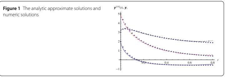
Figure 1The analytic approximate solutions and numeric solutions
Finally, we test the analytic approximate solutions and the numeric solutions for the system of the fractional differential equations
⎧ ⎪ ⎪ ⎨ ⎪ ⎪ ⎩
D0.7
t y1(t) = –2y1–y2–y3,
D0.5t y2(t) =y1–y2+y3+t,
D0.8
t y3(t) = –y2– 3y3+ 1,
(53)
subject to the initial conditions
y1(0) = 2, y2(0) = 3, y3(0) = 5.
From Eqs. (39), (40) and (41), the analytic approximate solutions y1[14](t), y[14]2 (t) and
y[14]3 (t) are calculated using the approximations of the first 14 terms, G[14](t) and Q[14](t).
The numeric solutionsy1,i,y2,iandy3,ifori= 1, 2, . . . , 40 with the step sizeh= 0.02 are given
by suing the scheme (52). We implement these algorithms by using MATHEMATICA 8. In Fig.1, the solid line, dot-dash line and dash line represent the analytic approximate solutionsy[14]1 (t),y2[14](t) andy[14]3 (t), respectively, and the dot lines denote the numeric so-lutionsy1,i,y2,iandy3,i. The consistence of the two solutions verifies the effectiveness of
our proposed analytic method.
5 Conclusions
The solutions of system of linear fractional differential equations of incommensurate or-ders are investigated in this paper. First, we introduce ann-variable Mittag–Leffler func-tion withn+ 1 parameters. Then we derive the analytic expressions for the solutions of the fractional system by using the Laplace transform and multi-variable Mittag–Leffler func-tions of matrix arguments. Finally, we verify the analytic result with numeric solufunc-tions by an example, where the numeric solutions are given by generalizing the L1 algorithm to the fractional system.
We generate the plots of analytic approximate solutions and numeric solutions with the help of MATHEMATICA 8. The obtained series solutions are convergent on the entire interval 0 <t< +∞and are easy to program and are approximated by any symbolic com-putation software.
Funding
This work was supported by the National Natural Science Foundation of China (No. 11772203).
Competing interests
Authors’ contributions
All authors read and approved the final manuscript.
Publisher’s Note
Springer Nature remains neutral with regard to jurisdictional claims in published maps and institutional affiliations.
Received: 16 February 2018 Accepted: 1 July 2018 References
1. Oldham, K.B., Spanier, J.: The Fractional Calculus. Academic, New York (1974)
2. Ross, B.: A brief history and exposition of the fundamental theory of fractional calculus. In: Ross, B. (ed.) Fractional Calculus and Its Applications (Lecture Notes in Mathematics, vol. 457, pp. 1–36. Springer, Berlin (1975)
3. Miller, K.S., Ross, B.: An Introduction to the Fractional Calculus and Fractional Differential Equations. Wiley, New York (1993)
4. Carpinteri, A., Mainardi, F. (eds.): Fractals and Fractional Calculus in Continuum Mechanics. Springer, Wien (1997) 5. Podlubny, I.: Fractional Differential Equations. Academic, San Diego (1999)
6. Kilbas, A.A., Srivastava, H.M., Trujillo, J.J.: Theory and Applications of Fractional Differential Equations. Elsevier, Amsterdam (2006)
7. Mainardi, F.: Fractional Calculus and Waves in Linear Viscoelasticity. Imperial College, London (2010) 8. Diethelm, K.: The Analysis of Fractional Differential Equations. Springer, Berlin (2010)
9. B˘aleanu, D., Diethelm, K., Scalas, E., Trujillo, J.J.: Fractional Calculus Models and Numerical Methods. Series on Complexity, Nonlinearity and Chaos. World Scientific, Boston (2012)
10. Baleanu, D., Jajarmi, A., Asad, J.H., Blaszczyk, T.: The motion of a bead sliding on a wire in fractional sense. Acta Phys. Pol. A131, 1561–1564 (2017)
11. Mainardi, F., Spada, G.: Creep, relaxation and viscosity properties for basic fractional models in rheology. Eur. Phys. J. Spec. Top.193, 133–160 (2011)
12. Li, M.: Three classes of fractional oscillators. Symmetry10, 40–91 (2018)
13. Mainardi, F.: Fractional relaxation-oscillation and fractional diffusion-wave phenomena. Chaos Solitons Fractals7, 1461–1477 (1996)
14. Metzler, R., Klafter, J.: The random walk’s guide to anomalous diffusion: a fractional dynamics approach. Phys. Rep.
339, 1–77 (2000)
15. Duan, J.S.: Time- and space-fractional partial differential equations. J. Math. Phys.46, 13504–13511 (2005)
16. Wu, G.C., Baleanu, D., Zeng, S.D., Deng, Z.G.: Discrete fractional diffusion equation. Nonlinear Dyn.80, 281–286 (2015) 17. Monje, C.A., Chen, Y.Q., Vinagre, B.M., Xue, D., Feliu, V.: Fractional-Order Systems and Controls, Fundamentals and
Applications. Springer, London (2010)
18. Baleanu, D., Jajarmi, A., Hajipour, M.: A new formulation of the fractional optimal control problems involving Mittag–Leffler nonsingular kernel. J. Optim. Theory Appl.175, 718–737 (2017)
19. Jajarmi, A., Hajipour, M., Mohammadzadeh, E., Baleanu, D.: A new approach for the nonlinear fractional optimal control problems with external persistent disturbances. J. Franklin Inst.355, 3938–3967 (2018)
20. Jajarmi, A., Hajipour, M., Baleanu, D.: New aspects of the adaptive synchronization and hyperchaos suppression of a financial model. Chaos Solitons Fractals99, 285–296 (2017)
21. Duan, J.S., Lu, L., Chen, L., An, Y.L.: Fractional model and solution for the Black–Scholes equation. Math. Methods Appl. Sci.41, 697–704 (2018)
22. Li, M., Lim, S.C., Chen, S.: Exact solution of impulse response to a class of fractional oscillators and its stability. Math. Probl. Eng.2011, 657839 (2011)
23. Li, C., Zeng, F.: Numerical Methods for Fractional Calculus. CRC Press, Boca Raton (2015)
24. Jafari, H., Khalique, C.M., Ramezani, M., Tajadodi, H.: Numerical solution of fractional differential equations by using fractional B-spline. Cent. Eur. J. Phys.11, 1372–1376 (2013)
25. Wu, G.C., Baleanu, D., Xie, H.P., Chen, F.L.: Chaos synchronization of fractional chaotic maps based on the stability condition. Physica A460, 374–383 (2016)
26. Machado, J.A.T., Baleanu, D., Luo, A.C.J. (eds.): Discontinuity and Complexity in Nonlinear Physical Systems. Springer, Cham (2014)
27. Cao, W., Xu, Y., Zheng, Z.: Existence results for a class of generalized fractional boundary value problems. Adv. Differ. Equ.348, 14 (2017)
28. Hajipour, M., Jajarmi, A., Baleanu, D.: An efficient nonstandard finite difference scheme for a class of fractional chaotic systems. J. Comput. Nonlinear Dyn.13, 021013 (2017)
29. Baleanu, D., Inc, M., Yusuf, A., Aliyu, A.I.: Lie symmetry analysis, exact solutions and conservation laws for the time fractional Caudrey–Dodd–Gibbon–Sawada–Kotera equation. Commun. Nonlinear Sci. Numer. Simul.59, 222–234 (2018)
30. Baleanu, D., Inc, M., Yusuf, A., Aliyu, A.I.: Space-time fractional Rosenou–Haynam equation: Lie symmetry analysis, explicit solutions and conservation laws. Adv. Differ. Equ.2018, 46 (2018)
31. Baleanu, D., Inc, M., Yusuf, A., Aliyu, A.I.: Time fractional third-order evolution equation: symmetry analysis, explicit solutions, and conservation laws. J. Comput. Nonlinear Dyn.13, 021011 (2018)
32. Inc, M., Yusuf, A., Aliyu, A.I., Baleanu, D.: Lie symmetry analysis, explicit solutions and conservation laws for the space-time fractional nonlinear evolution equations. Physica A496, 371–383 (2018)
33. Mainardi, F., Gorenflo, R.: On Mittag–Leffler-type functions in fractional evolution processes. J. Comput. Appl. Math.
118, 283–299 (2000)
34. Caputo, M., Fabrizio, M.: A new definition of fractional derivative without singular kernel. Prog. Fract. Differ. Appl.1, 73–85 (2015)
36. Atanackovic, T.M., Stankovic, B.: On a system of differential equations with fractional derivatives arising in rod theory. J. Phys. A37, 1241–1250 (2004)
37. Daftardar-Gejji, V., Babakhani, A.: Analysis of a system of fractional differential equations. J. Math. Anal. Appl.293, 511–522 (2004)
38. Deng, W., Li, C., Lü, J.: Stability analysis of linear fractional differential system with multiple time delays. Nonlinear Dyn.
48, 409–416 (2007)
39. Duan, J.S., Chaolu, T., Sun, J.: Solution for system of linear fractional differential equations with constant coefficients. J. Math.29, 599–603 (2009)
40. Duan, J.S., Fu, S.Z., Wang, Z.: Solution of linear system of fractional differential equations. Pac. J. Appl. Math.5, 93–106 (2013)
41. Charef, A., Boucherma, D.: Analytical solution of the linear fractional system of commensurate order. Comput. Math. Appl.62, 4415–4428 (2011)
42. Odibat, Z.M.: Analytic study on linear systems of fractional differential equations. Comput. Math. Appl.59, 1171–1183 (2010)
43. Daftardar-Gejji, V., Jafari, H.: Adomian decomposition: a tool for solving a system of fractional differential equations. J. Math. Anal. Appl.301, 508–518 (2005)
44. Gaboury, S., Özarslan, M.A.: Singular integral equation involving a multivariable analog of Mittag–Leffler function. Adv. Differ. Equ.2014, 252 (2014)
45. Jaimini, B.B., Gupta, J.: On certain fractional differential equations involving generalized multivariable Mittag–Leffler function. Note Mat.32, 141–156 (2012)