Computation of eigenvalues of discontinuous dirac system using Hermite interpolation technique

R E S E A R C H

Open Access

Computation of eigenvalues of discontinuous

dirac system using Hermite interpolation

technique

Mohammed M Tharwat

and Ali H Bhrawy

* Correspondence: [email protected]

1_{Department of Mathematics,}

Faculty of Science, King Abdulaziz University, Jeddah, Saudi Arabia Full list of author information is available at the end of the article

Abstract

We use the derivative sampling theorem (Hermite interpolations) to compute eigenvalues of a discontinuous regular Dirac systems with transmission conditions at the point of discontinuity numerically. We closely follow the analysis derived by Levitan and Sargsjan (1975) to establish the needed relations. We use recently derived estimates for the truncation and amplitude errors to compute error bounds. Numerical examples, illustrations and comparisons with the sinc methods are exhibited.

Mathematical Subject Classification 2010:34L16; 94A20; 65L15.

Keywords:Dirac systems, Hermite interpolations, transmission conditions, discontinu-ous boundary value problems, truncation and amplitude errors, sinc methods

1 Introduction Lets> 0 andPW2

σbe the Paley-Wiener space of allL2(ℝ)-entire functions of exponen-tial type types. Assume that f(t)∈PW_σ2 ⊂PW2_2σ. Thenf(t) can be reconstructed via the sampling series

f(t) = ∞

n=−∞

f

_nπ σ

S2_n(t) +f

_nπ σ

_{sin(σt−nπ)} σ Sn(t)

, (1)

whereSn(t) is the sequences of sinc functions

Sn(t) := ⎧ ⎪ ⎨ ⎪ ⎩

sin(σt−nπ) (σt−nπ) ,t=

nπ

σ ,

1, t= nπ

σ .

(2)

Series (1) converges absolutely and uniformly onℝ(cf. [1-4]). Sometimes, series (1) is called the derivative sampling theorem. Our task is to use formula (1) to compute eigenvalues of Dirac systems numerically. This approach is a fully new technique that uses the recently obtained estimates for the truncation and amplitude errors associated with (1) (cf. [5]). Both types of errors normally appear in numerical techniques that use interpolation procedures. In the following we summarize these estimates. The truncation error associated with (1) is defined to be

RN(f)(t) :=f(t)−fN(t), N∈Z+, t∈R, (3) wherefN(t) is the truncated series

fN(t) =

σandf(t) is sufficiently smooth in the sense that there existskÎℤ+such thattkf(t)Î L2(ℝ), then, fortÎℝ, |t| <Nπ/s, we have

The amplitude error occurs when approximate samples are used instead of the exact ones, which we can not compute. It is defined to be

A(ε,f)(t) =

respectively. Let us assume that the differences

εn:=f

The classical [6] sampling theorem of Whittaker, Kotel’nikov and Shannon (WKS) for f ∈PW2_σis the series representation

f(t) = ∞

n=−∞

fnπ

σ

Sn(t), t∈R, (12)

where the convergence is absolute and uniform on ℝand it is uniform on compact sets ofℂ(cf. [6-8]). Series (12), which is of Lagrange interpolation type, has been used to compute eigenvalues of second order eigenvalue problems (see e.g. [9-13]). The use of (12) in numerical analysis is known as the sinc-method established by Stenger (cf. [14-16]). In [11,12], the authors applied (12) and the regularized sinc method to com-pute eigenvalues of Dirac systems with a derivation of the error estimates as given by [17,18]. The regularized sinc method; a method which is based on (WKS) but applied to regularized functions. Hence avoiding any (multiple) integration and keeping the number of terms in the Cardinal series manageable. It has been demonstrated that the method is capable of delivering higher order estimates of the eigenvalues at a very low cost. The aim of this article is to investigate the possibilities of using Hermite interpo-lations rather than Lagrange interpointerpo-lations, to compute the eigenvalues numerically. Notice that, due to Paley-Wiener’s theorem [19]f ∈PW2_σif and only if there isg(·)ÎL2

(-s,s) such that

f(t) = √1 2π

σ

−σ

g(x)eixtdx. (13)

Therefore f(t)∈PW2_σ,i.e,f′(t) also has an expansion of the form (12). However,f′(t) can be also obtained by term-by-term differentiation formula of (12)

f(t) = ∞

n=−∞

fnπ

σ

S_n(t), (14)

see [[6], p. 52] for convergence. Thus the use of Hermite interpolations will not cost any additional computational efforts since the samples fn_σπwill be used to compute bothf(t) andf′(t) according to (12) and (14), respectively. We would like to mention that works in direction of computing eigenvalues with the new method, Hermite interpola-tion technique, are few (see e.g. [5]). Also articles in computing of eigenvalues with dis-continuous are few (see [20-22]). However the computing of eigenvalues by Hermite interpolation technique which has discontinuity conditions, do not exist as for as we know. The next section contains some preliminary results. The method with error esti-mates are contained in Section three. The last section involves some illustrative examples.

2 The eigenvalue problem

In this section we closely follow the analysis derived by [23] to establish the needed relations (see also [24]). We consider the Dirac system

u₂(x)−r1(x)u1(x) =λu1(x), u1(x) +r2(x)u2(x) =−λu2(x), x∈[−1, 0)∪(0, 1], (15)

U2(u) := sinβu1(1) + cosβu2(1) = 0, (17)

Let Hbe the Hilbert space

H :=

The inner product ofHis defined by

u(·),v(·)H:=

where⊤denotes the matrix transpose,

u(x) =

Equation (15) can be written as

(u) :=Au(x)−P(x)u(x) =λu(x), (22)

In the following lemma, we will prove that the eigenvalues of the problem (15)-(19) are real.

Lemma 2.1The eigenvalues of the problem(15)-(19)are real.

Proof. Assume the contrary thatl0is a nonreal eigenvalue of problem (15)-(19). Let

u1(x)

u2(x)

be a corresponding (non-trivial) eigenfunction. By (15), we have, forxÎ[−1, 0)

⋃(0, 1],

d

dx{u1(x)u¯2(x)− ¯u1(x)u2(x)}= (λ¯0−λ0){|u1(x)|

Integrating the above equation through [−1, 0) and (0, 1], we obtain

(λ¯0−λ0) ⎡ ⎣

0

−1

(|u1(x)|2+|u2(x)|2)dx ⎤

⎦=u1(0−)u¯2(0−)− ¯u1(0−)u2(0−)

−[u1(−1)u¯2(−1)− ¯u1(−1)u2(−1)], (25)

(λ¯0−λ0) ⎡ ⎣

1

0

(|u1(x)|2+|u2(x)|2)dx ⎤

⎦=u1(1)u¯2(1)− ¯u1(1)u2(1)

−[u1(0+)u¯2(0+)− ¯u1(0+)u2(0+)].

(26)

Then from (16), (17) and transmission conditions, we have respectively

u1(−1)u¯2(−1)− ¯u1(−1)u2(−1) = 0,

u1(1)u¯2(1)− ¯u1(1)u2(1) = 0 and

u1(0−)u¯2(0−)− ¯u1(0−)u2(0−) =δ2[u1(0+)u¯2(0+)− ¯u1(0+)u2(0+)]. Since _λ0=λ¯0,it follows from the last three equations and (25), (26) that

0

−1

(|u1(x)|2+|u2(x)|2)dx+δ2 1

0

(|u1(x)|2+|u2(x)|2)dx= 0. (27)

Then ui(x) = 0,i=1, 2 and this is contradiction. Consequently,l0must be real.

Lemma 2.2 Letl1andl2be two different eigenvalues of the problem(15)-(19).Then the corresponding eigenfunctionsu(x,l1)andv(x,l2)of this problem satisfy the follow-ing equality

0

−1

u(x, λ1)v(x, λ2)dx+δ2 1

0

u(x, λ1)v(x, λ2)dx= 0. (28)

Proof. By (15) we obtain

d

dx{u1(x,λ1)v2(x,λ2)−u2(x,λ2)v1(x,λ1)}= (λ2−λ1){u1(x,λ1)v1(x,λ2)+u2(x, λ1)v2(x, λ2)}.

Integrating the above equation through [−1, 0) and (0, 1], and taking into account u (x,l1) andv(x,l2) satisfy (16)-(19), we obtain (28), wherel1≠l2.

Now, we shall construct a special fundamental system of solutions of the Equation (15) for lnot being an eigenvalue. Let us consider the next initial value problem:

u₂(x)−r1(x)u1(x) =λu1(x), u

1(x) +r2(x)u2(x) =−λu2(x), x∈(−1, 0), (29)

u1(−1) = cosα, u2(−1) =−sinα. (30) By virtue of Theorem 1.1 in [23] this problem has a unique solution

entire function of l Î ℂ for each fixedx Î [−1, 0]. Similarly, employing the same method as in proof of Theorem 1.1 in [23], we see that the problem

u₂(x)−r1(x)u1(x) =λu1(x), u1(x) +r2(x)u2(x) =−λu2(x), x∈(0, 1), (31)

u1(1) = cosβ, u2(1) =−sinβ. (32)

has a unique solutionu=

χ12(x,λ) χ22(x,λ)

which is an entire function of parameterlfor

each fixedxÎ [0.1].

Now the functions i2(x, l) andci1(x,l) are defined in terms ofi1(x,l) andci2(x,

l),i=1, 2, respectively, as follows: The initial-value problem,

u₂(x)−r1(x)u1(x) =λu1(x), u1(x) +r2(x)u2(x) =−λu2(x), x∈(0, 1), (33)

u1(0) = 1

δφ11(0, λ), u2(0) = 1

δφ21(0, λ), (34)

has unique solutionu=

φ12(x,λ) φ22(x,λ)

for eachlÎℂ.

Similarly, the following problem also has a unique solutionu=

χ11(x,λ) χ21(x,λ)

:

u2(x)−r1(x)u1(x) =λu1(x), u1(x) +r2(x)u2(x) =−λu2(x), x∈(−1, 0), (35)

u1(0) =δχ12(0, λ), u2(0) =δχ22(0, λ). (36) Let us construct two basic solutions of the equation (15) as

φ(·, λ) =

φ1(·, λ) φ2(·, λ)

, X(·, λ) =

X1(·, λ) X2(·, λ)

,

where

φ1(x, λ) =

φ11(x, λ),x∈[−1, 0)

φ12(x, λ),x∈(0, 1] , φ2(x, λ) =

φ21(x, λ),x∈[−1, 0) φ22(x, λ),x∈(0, 1] , (37)

χ1(x, λ) =

χ11(x, λ),x∈[−1, 0)

χ12(x, λ),x∈(0, 1] , χ2(x, λ) =

χ21(x, λ),x∈[−1, 0) χ22(x, λ),x∈(0, 1] , (38) By virtue of Equations (34) and (36) these solutions satisfy both transmission condi-tions (18) and (19). These funccondi-tions are entire inlfor allxÎ[−1, 0)⋃(0, 1].

Let W(,c)(·,l) denote the Wronskian of(·,l) andc(·,l) defined in [[25], p. 194], i.e.,

W(φ, χ)(·, λ) :=φ1(·,λ)φ2(·,λ)

χ1(·,λ)χ2(·,λ) .

It is obvious that the Wronskian

i(λ) :=W(φ, χ)(x, λ) =φ1i(x, λ)χ2i(x, λ)−φ2i(x, λ)χ1i(x, λ), x∈i, i= 1, 2 (39)

are independent of xÎ Γi and are entire functions. Taking into account (34) and

1(λ) =δ22(λ), for eachlÎℂ.

Corollary 2.3The zeros of the functionsΩ1(l)andΩ2(l)coincide.

Then, we may introduce to the consideration the characteristic function Ω(l) as

(λ) :=1(λ) =δ22(λ). (40)

In the following lemma, we show that all eigenvalues of the problem (15)-(19) are simple.

Lemma 2.4All eigenvalues of problem(15)-(19)are just zeros of the function Ω(l).

Moreover, every zero ofΩ(l)has multiplicity one.

Proof. Since the functions1(x,l) and2(x,l) satisfy the boundary condition (16)

and both transmission conditions (18) and (19), to find the eigenvalues of the (15)-(19) we have to insert the functions 1(x,l) and 2(x, l) in the boundary condition (17)

and find the roots of this equation. By (15) we obtain for l,µÎℂ,l≠μ,

d

dx{φ1(x, λ)φ2(x, μ)−φ1(x, μ)φ2(x, λ)}= (μ−λ){φ1(x, λ)φ1(x, μ)+φ2(x, λ)φ2(x, μ)}.

Integrating the above equation through [−1, 0) and (0, 1], and taking into account the initial conditions (30), (34) and (36), we obtain

φ12(1, λ)φ22(1, μ)−φ12(1, μ)φ22(1, λ) =

(μ−λ)

⎛ ⎝

0

−1

(φ11(x, λ)φ11(x, μ) +φ21(x, λ)φ21(x, μ))dx

+δ2 1

0

(φ12(x, λ)φ12(x, μ) +φ22(x, λ)φ22(x, μ))dx ⎞ ⎠.

(41)

Dividing both sides of (41) by (l−µ) and by lettingµ®l, we arrive to the relation

φ22(1,λ)∂φ 12(1,λ)

∂λ −φ12(1,λ) ∂φ 22(1,λ)

∂λ =−

⎛ ⎝

0

−1

|φ11(x,λ)2 + φ21(x,λ)|2

dx

+δ2 1

0

|φ12(x,λ)2+φ22(x,λ)|2

dx

⎞ ⎠.

(42)

We show that equation

(λ) =−δ2(sinβφ12(1, λ) + cosβφ22(1, λ)) = 0 (43) has only simple roots. Assume the converse, i.e., Equation (43) has a double rootl*, say. Then the following two equations hold

sinβφ12(1, λ∗) + cosβφ22(1, λ∗) = 0, (44)

sinβ∂φ12(1,λ ∗₎ ∂λ + cosβ

∂φ22(1,λ∗)

The Equations (44) and (45) imply that

φ22(1, λ∗)∂φ12 (1,λ∗)

∂λ −φ12(1, λ∗)∂φ22 (1,λ∗)

∂λ (46)

Combining (46) and (42), withl=l*, we obtain

0

−1

(|φ11(x, , λ∗)|2+|φ21(x, , λ∗)|2)dx+δ2 1

0

(|φ12(x, , λ∗)|2+|φ22(x, , λ∗)|2)dx= 0. (47)

It follows that 1(x,l*)=2(x,l*)=0, which is impossible. This proves the lemma.

Here{φ(·, λn)}∞n=−∞will be a sequence of eigen-vector-functions of (15)-(19) corre-sponding to the eigenvalues{λn}∞n=−∞.Sincec(·,l) satisfies (17)-(19), then the eigenva-lues are also determined via

sinαχ11(−1, λ) + cosαχ21(−1,λ) =(λ). (48) Therefore{χ(·, λn)}∞n=−∞is another set of eigen-vector-functions which is related by {φ(·, λn)}∞n=−∞with

χ(x, λn) =cnφ(x, λn), x∈[−1, 0)∪(0, 1], n∈Z, (49)

Where cn≠ 0 are non-zero constants, since all eigenvalues are simple. Since the eigenvalues are all real, we can take the eigen-vector-functions to be real valued.

Since (·,l) satisfies (16), then the eigenvalues of the problem (15)-(19) are the zeros of the function

(λ) =−δ2(sinβφ12(1, λ) + cosβφ22(1, λ)). (50) Notice that both (·, l) andΩ(l) are entire functions ofl. Now we shall transform Equations (15), (30), (34) and (37) into the integral equations (see [25]),

φ11(x, λ) = cos(λ(x+ 1)−α)−S−1,1φ11(x, λ)− ˜S−1,2φ21−(x, λ), (51)

φ21(x, λ) = sin(λ(x+ 1)−α) +S˜−1,1φ11(x, λ)−S−1,2φ21(x, λ), (52)

φ12(x, λ) =

1

δφ11(0−,λ) cos(λx)−

1

δφ21(0−, λ) sin(λx)−S0,1φ12(x,λ)− ˜S0,2φ22(x, λ), (53)

φ22(x,λ) =

1

δφ11(0−,λ) sin(λx)+

1

δφ21(0−, λ) cos (λx)−+S˜0,1φ12(x, λ)−S0,2φ22(x, λ), (54)

where_S−1,i, S˜−1,i, S0,iandS˜0,i, i= 1, 2,are the Volterra integral operators defined by

S−1,iϕ(x, λ) := x

−1

sinλ(x−t)ri(t)ϕ(t, λ)dt, S−˜ 1,iϕ(x, λ) := x

−1

cosλ(x−t)ri(t)ϕ(t, λ)dt,

S0,iϕ(x, λ) := x

0

sinλ(x−t)ri(t)ϕ(t, λ)dt, S˜0,iϕ(x, λ) := x

0

For convenience, we define the constants

c1:= 0

−1

[|r1(t)|+|r2(t)|]dt, c2:=c1exp(c1),

c3:= 1

0

[|r1(t)|+|r2(t)|]dt, c4:=c2+ 2

|δ|(1 +c2).

(55)

Defineh−1,i(·,l) andh0,i(·,l),i= 1, 2, to be

h₋1,1(x,λ) :=S−1,1φ11(x,λ) +S˜−1,2φ21(x,λ),

h−1,2(x,λ) :=S˜−1,1φ11(x,λ) +S−1,2φ21(x,λ), %

(56)

h0,1(x,λ) :=S0,1φ12(x,λ) +S˜0,2φ22(x,λ),

h0,2(x,λ) :=S˜0,1φ12(x,λ)−S0,2φ22(x,λ). %

(57)

Lemma 2.5The functions h₋1,1(x,l)and h−1,2(x,l)are entire inlfor any fixed xÎ

[−1, 0)and satisfy the growth condition

|h−1,1(x, λ)|, |h−1,2(x, λ)| ≤2c2e|λ|(x+1), λ∈C. (58) Proof. Sinceh−1,1(x, λ) =S−1,1φ11(x, λ) +S˜−1,2φ21(x, λ),then from (51) and (52) we obtain h−1,1(x, λ) =S−1,1cos(λ(x+1)−α)+S−˜ 1,2sin(λ(x+1)−α)−S−1,1h−1,1−(x,λ)+S−˜ 1,2h−1,2(x,λ)

Using the inequalities_|sinz| ≤e|z|_{and|cosz| ≤e}|z|_{forz∈C,leads for}lÎℂ_to

|h−1,1(x,λ)| ≤ |S−1,1cos(λ(x+ 1)−α)|+| ˜S−1,2sin(λ(x−+1)−α)|+|S−1,1h−1,1(x,λ)|

+| ˜S−1,2h−1,2(x, λ)|

≤e|λ|(x+1)

x

−1

[|r1(t)||h−1,1(t, λ)|+|r2(t)||h−1,2(t, λ)|]e−|λ|(t+1)dt

+ 2e|λ|(x+1)

x

−1

[|r1(t)|+|r2(t)|]dt

≤2c1e|λ|(x+1)+e|λ|(x+1)

x

−1

[|r1(t)||h−1,1(t, λ)|+|r2(t)||h−1,2(t, λ)|]e−|λ|(t+1)dt.

The above inequality can be reduced to

e−|λ|(x+1)_|h

−1,1(x,λ)| ≤2c1+

x

−1

[|r1(t)||h−1,1(t, λ)|+|r2(t)||h−1,2(t,λ)|]e−|λ|(t+1)dt. (59)

Similarly, we can prove that

e−|λ|(x+1)_|h

−1,2(x,λ)| ≤2c1+

x

−1

[|r1(t)||h−1,1(t, λ)|+|r2(t)||h−1,2(t,λ)|]e−|λ|(t+1)dt. (60)

|h0,1(x, λ)|,|h0,2(x, λ)| ≤2c3c4e|λ|(x+1), λ∈C. (61) Proof. Sinceh0,1(x, λ) =S0,1φ11(x, λ) +S˜0,2φ21(x, λ),then from (53) and (54) we obtain

h0,1(x, λ) = 1

δφ11(0−, λ)S0,1cos(λx)− 1

δφ21(0−, λ)S˜0,1sin(λx)−S0,1h−1,2(x, λ) +1

δφ11(0−, λ)S˜0,2sin(λX) +1

δφ21(0−, λ)S˜0,2cos(λX) +S˜0,2h−1,2(x, λ).

Then from (51) and (52) and Lemma 2.5, we get

h0,1(x, λ)≤ 1

|δ||φ11(0−, λ)||S0,1cos(λx)|+ 1

|δ||φ21(0−, λ)||S0,1sin(λx)| +|S0,1h−1,2(x, λ)|+

1

|δ||φ11(0−, λ)|| ˜S0,2sin(λx)| + 1

|δ||φ21(0−, λ)|| ˜S0,2cos(λx)| −+| ˜S0,2h−1,2(x, λ)| ≤2

c2+ 2

|δ|(1 +c2)

c3e|λ|(x+1)= 2c3c4e|λ|(x+1).

Similarly, we can prove that

h0,2(x, λ)≤2c3c4e|λ|(x+1).

3 The numerical scheme

In this section we derive the method of computing eigenvalues of problem (15)-(19) numerically. The basic idea of the scheme is to splitΩ(l) into two parts a known part

K(λ)and an unknown one U(λ). Then we prove that U(λ)has an expansion of the form (1). We then approximate U(λ)in two stages. First by truncating the sampling expansion (4) and then by approximating the samples, using standard methods of sol-ving ordinary differential equations. This produces both a truncation error and an amplitude error. We apply forms (4) and (7) to derive an estimate of the error of the technique. We first splitΩ(l) into two parts:

(λ) :=K(λ) +U(λ), (62)

whereU(λ)is the unknown part involving integral operators

U(λ) :=δ2sinβh0,1(1,λ)−δ2cosβh0,2(1,λ)−δsin(λ−β)h−1,1(0−,λ)−δcos(λ+β)h−1,2(0−,λ), (63)

andK(λ)is the known part

K(λ) :=−δsin(2λ−α+β). (64)

Then, from Lemmas 2.5 and 2.6, we have the following result.

Lemma 3.1The function U(λ)is entire inland the following estimate holds

|U(λ)| ≤Me2|λ|_{, (65)}

where

Proof. From (63), we have

Lemma 3.2Gθ,m(λ)is an entire function oflwhich satisfies the estimate |Gθ,m(λ)| ≤

A direct and important result of Lemma 51 is thatGθ,m(λ)belongs to the Paley-Wie-nerz space PW2

σwith s = 1+mθ. SinceGθ,m(λ)∈PW2_σ ⊂PW22σ,then we can recon-struct the functionsGθ,m(λ)via the following sampling formula

Let NÎ ℤ+,N>mand approximateGθ,m(λ)by its truncated seriesGθ,m,N(λ), where

Since all eigenvalues are real, then from now on we restrict ourselves tolÎℝ. Since

λm−1_G

in general, are not known

explicitly. So we approximate them by solving numerically 2N+ 1 initial value

pro-blems at the nodesnπ approximations of the samples ofG_θ,m

_nπ

Using standard methods for solving initial problems, we may assume that for |n| <N,

In the following we use the technique of [27] to determine enclosure intervals for the eigenvalues. Letl*be an eigenvalue, that is

Then it follows that has computable upper bound, we can define an enclosure forl*, by solving the follow-ing system of inequalities

Its solution is an interval containing l*, and over which the graph

K(λ∗) +

uniformly over any compact set, and since l* is a simple root, we obtain for largeN

and in particularl*ÎIε,N. Summarizing the above discussion, we arrive at the follow-ing lemma which is similar to that of [27] for Sturm-Liouville problems.

Lemma 3.3For any eigenvaluel*,we can find N0Î ℤ+ and sufficiently smallεsuch thatl*ÎI_ε,Nfor N>N0.Moreover

[a₋(λ∗, N, ε), a+(λ∗, N, ε)]→ {λ∗}asN→ ∞andε→0. (84) Proof. Since all eigenvalues of (15)-(19) are simple, then for largeNand sufficiently

small ε we have ∂

|(λN)−(λ∗)| ≤ sinθλN

θλN

−m(TN,m−1,σ(λN) +A(ε)). (87)

Using the mean value theorem yields that for some ζÎJ_ε,N:=[min(l*, lN), max(l*,

lN)],

|(λ∗−λN)(ζ)| ≤ sinθλN

θλN

−m(TN,m−1,σ(λN) +A(ε)), ζ ∈Jε,N ⊂Iε,N. (88)

Since the eigenvalues are simple, then for sufficiently large N_ζinf_∈I ε,N|

_(ζ)|>0 and

we get (86).

4 Numerical examples

This section includes two detailed worked examples illustrating the above technique. By ESandEHwe mean the absolute errors associated with the results of the classical sinc method and our new method (Hermite interpolations) respectively. All examples are computed in [22] with the classical sinc method. We indicate in these examples the effect of the amplitude error in the method by determining enclosure intervals for different values ofε. We also indicate the effect of the parameters mandθ by several choices. Every example is accompanied with six figures illustrating(λ),˜(λ)and the enclosure curves dominating the zeros. Recall that a±(l) are defined by

a±(λ) =N(λ)±

sin_θλθλ−m(TN,m−1,σ(λ) +A(ε)), |λ| < N_σπ. (89)

Recall also that the enclosure interval Iε,N:=[a-,a+] is determined by solving

a±(λ) = 0,|λ|< Nπ

σ . (90)

Example 1Consider the system

u2(x)−r(x)u1(x) =λu1(x), u1(x) +r(x)u2(x) =−λu2(x), x∈[−1, 0)∪(0, 1], (91)

u1(–1) +u2(–1) = 0, u1(1) +u2(1) = 0, (92)

u1(0−)−2u1(0+) = 0, u2(0−)−2u2(0+) = 0. (93)

Here

r1(x) =r2(x) =r(x) =

x2,x∈[−1, 0)

x, (0, 1], (94)

α=β = π

4 andδ= 2.Direct calculations give

K(λ) =−2 sin[2λ] (95)

and

(λ) =−2 sin

5 6+ 2λ

therefore the eigenvalues are_λk=6kπ−5

12 ,k∈Z.The following four tables indicate

the application of our technique to this problem and the effect of ε, θand m (Tables1, 2, 3and4).

In the following, the Figures1and2illustrate the comparison betweenΩ(l)and˜N(λ)

for different values of m andθ.

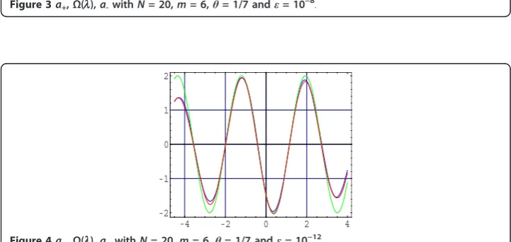
Figures 3 and 4, for N = 20, m = 6 andθ= 1/7, illustrate the enclosure intervals for

ε= 10−8 andε= 10−12respectively.

Also, Figures 5 and 6illustrate the enclosure intervals for ε= 10−8 and ε= 10−12

respectively, but for m= 10,θ=1/5.

Table 1N= 20,m= 6, andθ= 1/7

lkSinclk,N Exactlk Hermitelk,N ES EH l−2−3.558259424986099 −3.5582593202564599 −3.5582593202488253 1.047×10−

7

7.634×10−12

l−1−1.9874629152275372 −1.9874629934615633 −1.9874629934659096 7.823×10− 8

4.346×10−12

l0−0.4166665411688605 −0.4166666666666667 −0.41666666665625623 1.255×10−7 1.041×10−11

l11.1541296373132959 1.1541296601282299 1.1541296601279385 2.281×10−8 2.913×10−13 l22.7249258102486835 2.7249259869231266 2.7249259869365776 1.767×10−7 1.345×10−11

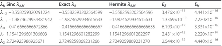
Table 2N= 20,m= 10 andθ= 1/5

lkSinclk,N Exactlk Hermitelk,N ES EH l−2−3.558259320291224 −3.5582593202564599 −3.5582593202564596 3.476×10−

11

4.441×10−16

l−1−1.9874629934481942 −1.9874629934615633 −1.9874629934615631 1.3369×10−11 2.220×10−16 l0−0.416666666672866 −0.4166666666666667 −0.41666666666666635 6.199×10−12 3.331×10−16 l11.1541296601306603 1.1541296601282299 1.1541296601282297 2.431×10−12 2.220×10−16 l22.724925986925671 2.7249259869231266 2.7249259869231270 2.544×10−12 4.440×10−16

Table 3 The approximationl_k,Nand the exact solutionlkare all inside the interval [a−,

a+] for different values ofε, whereN= 20,m= 6,θ= 1/7

lkExactlk [a−,a+],ε= 10− 8

[a−,a+],ε= 10− 12

lk,N

l−2−3.5582593202564599 [−3.753326,−3.387861] [−3.565657,−3.551497] −3.5582593202488253 l−1−1.9874629934615633 [−2.134039,−1.835158] [−1.991487,−1.983156] −1.9874629934659096 l0−0.4166666666666667 [−0.562608,−0.277479] [−0.427095,−0.406713] −0.41666666665625623 l11.1541296601282299 [1.017775, 1.295214] [1.153811, 1.154454] 1.1541296601279385 l22.7249259869231266 [2.561929, 2.895812] [2.711312, 2.738729] 2.7249259869365776 E5(Gθ,m) = 1.7659×106,E4(Gθ,m) = 278897,= 1,MGθ,m = 4563.57

Table 4 ForN= 20,m= 10 andθ= 1/5,l_k,Nandlkare all inside the interval [a−,a+] for

different values ofε

lkExactlk [a−,a+],ε= 10− 8

[a−,a+],ε= 10− 12

lk,N

l−2−3.5582593202564599 [−3.739980,−3.404715] [−3.560364,−3.556152] −3.5582593202564596 l−1−1.9874629934615633 [−2.080163,−1.899068] [−1.988611,−1.986313] −1.9874629934615631 l0−0.4166666666666667 [−0.487002,−0.346801] [0.417553,−0.415779] −0.41666666666666635 l11.1541296601282299 [1.079274, 1.230862] [1.153170, 1.155090] 1.1541296601282297 l22.7249259869231266 [2.614866, 2.845166] [2.723467, 2.726388] 2.7249259869231270

-4 -2 0 2 4 -2

-1 0 1 2

Figure 1Ω(l),˜_N(λ)withN= 20,m= 6 andθ= 1/7.

-4 -2 0 2 4

-2 -1 0 1 2

Figure 2Ω(l),˜_N(λ₎withN= 20,m= 10 andθ= 1/5.

-4 -2 0 2 4

-2 -1 0 1 2

Figure 3_a+,Ω(l),a-withN= 20,m= 6,θ= 1/7 andε= 10−8.

-4 -2 0 2 4

-2 -1 0 1 2

Example 2In this example we consider the system

u2(x)−r(x)u1(x) =λu1(x), u1(x) +r(x)u2(x) =−λu2(x), x∈[−1, 0)∪(0, 1], (97)

√

3u1(−1) +u2(−1) = 0, u1(1) + √

3u2(1) = 0, (98)

u1(0−)−3u1(0+) = 0, u2(0−)−3u2(0+) = 0, (99)

where

r1(x) =r2(x) =r(x) =

x, x∈[−1, 0)

x2_{+ 1, (0, 1],} (100)

α= π 3,β =

π

6andδ= 3.Direct calculations give

K(λ) = 3 sinπ 6 −2λ

+

(101)

and

(λ) = 3 2

cos

5 6 + 2λ

−√3 sin

5 6+ 2λ

, (102)

therefore the eigenvalues are _λk= (6k+ 1)π−5

12 ,k∈Z.As in the previous example,

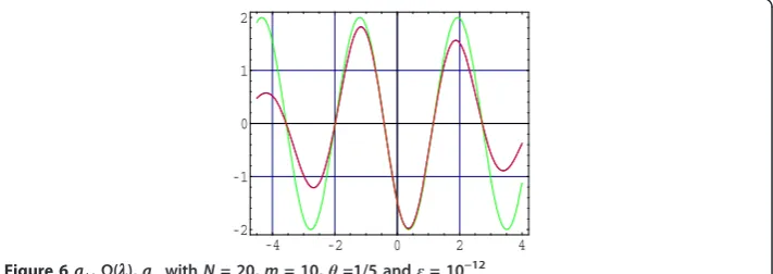
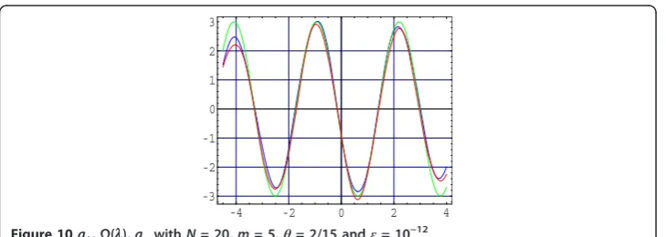
Figures 7, 8, 9, 10, 11and12illustrate the results of Tables 5, 6, 7and 8.Also,Figures

5and6illustrate the enclosure intervals forε= 10−8 andε= 10−12 respectively, but for m= 9,θ= 2/11.

-4 -2 0 2 4

-2 -1 0 1 2

Figure 5a+,Ω(l),a−withN= 20,m= 10,θ= 1/5 andε= 10−8.

-4 -2 0 2 4

-2 -1 0 1 2

-4 -2 0 2 4 -3

-2 -1 0 1 2 3

Figure 7Ω(l),˜_N(λ)withN= 20,m= 5 andθ= 2/15.

-4 -2 0 2 4

-3 -2 -1 0 1 2 3

Figure 8Ω(l),˜_N(λ₎withN= 20,m= 9 andθ= 2/11.

-4 -2 0 2 4

-3 -2 -1 0 1 2 3

Figure 9a+,Ω(l),a−withN= 20,m= 5,θ= 2/15 andε= 10−8.

-4 -2 0 2 4

-3 -2 -1 0 1 2 3

-4 -2 0 2 4 -3

-2 -1 0 1 2 3

Figure 11a+,Ω(l),a−withN= 20,m= 9,θ= 2/11 andε= 10−8.

-4 -2 0 2 4

-3 -2 -1 0 1 2 3

Figure 12a+,Ω(l),a−withN= 20,m= 9,θ= 2/11 andε= 10−12.

Table 5N= 20,m= 5,θ= 2/15

lkSinc_lk,N Exact_lk Hermite_lk,N ES EH l−2−3.2964601812375145 −3.2964599324573105 −3.2964599325093795 2.488×10−7 5.207×10−11 l−1−1.725663818527078 −1.725663605662414 −1.7256636055362218 2.129×10−7 1.262×10−10 l0−0.15486730070281368 −0.15486727886751722 −0.15486727888681906 2.183×10−8 _1.930×10−11 l11.4159289890168527 1.4159290479273794 1.4159290479703164 5.891×10−8 _4.294×10−11 l22.9867250912171013 2.986725374722276 2.9867253745880475 2.835 × 10−7 1.342×10−10

Table 6N= 20,m=9,θ=2/11

lkSinc_lk,N Exact_lk Hermite_lk,N ES EH l−2−3.2964599325179624 −3.2964599324573105 −3.2964599324573127 6.065 × 10−11 2.220×10−15 l−1−1.7256636056618686 −1.725663605662414 −1.725663605662413 5.453 × 10−13 8.881×10−16 l0−0.1548672788373793 −0.15486727886751722 −0.1548672788675186 3.013×10−11 _1.388×10−15 l11.415929047873631 1.4159290479273794 1.4159290479273827 5.374×10−11 _3.331×10−15 l22.986725374801227 2.986725374722276 2.9867253747222686 7.895×10−11 7.549×10−15

Table 7 ForN= 20,m=5 andθ= 2/15, the approximationl_k,Nand the exact solutionlk

are all inside the interval [a₋,a+] for different values ofε

lkExactlk [a−,a+],ε= 10−5 [a−,a+],ε= 10−10 lk,N

l−2−3.2964599324573105 [−3.402745,−3.177441] [−3.305475,−3.286114] −3.2964599325093795 l−1−1.725663605662414 [−1.840530,−1.615062] [−1.749858,−1.702197] −1.7256636055362218 l0−0.15486727886751722 [−0.250393,−0.067671] [−0.158786,−0.151287] −0.15486727888681906

l11.4159290479273794 [1.323736, 1.520703] [1.408023, 1.424863] 1.4159290479703164

l22.986725374722276 [2.863300, 3.109311] [2.960260, 3.012514] 2.9867253745880475

Acknowledgements

This article was funded by the Deanship of Scientific Research (DSR), King Abdulaziz University, Jeddah. The authors, therefore, acknowledge with thanks DSR technical and financial support.

Author details

1

Department of Mathematics, Faculty of Science, King Abdulaziz University, Jeddah, Saudi Arabia2Department of Mathematics, Faculty of Science, Beni-Suef University, Beni-Suef, Egypt

Authors’contributions

The authors have equal contributions to each part of this article. All the authors read and approved the final manuscript.

Competing interests

The authors declare that they have no competing interests.

Received: 20 March 2012 Accepted: 10 May 2012 Published: 10 May 2012

References

1. Grozev, GR, Rahman, QI: Reconstruction of entire functions from irregularly spaced sample points. Canad J Math.48, 777_–793 (1996). doi:10.4153/CJM-1996-040-7

2. Higgins, JR, Schmeisser, G, Voss, JJ: The sampling theorem and several equivalent results in analysis. J Comput Anal Appl.2, 333_–371 (2000)

3. Hinsen, G: Irregular sampling of bandlimitedLp-functions. J Approx Theory.72, 346–364 (1993). doi:10.1006/ jath.1993.1027

4. Jagerman, D, Fogel, L: Some general aspects of the sampling theorem. IRE Trans Inf Theory.2, 139–146 (1956). doi:10.1109/TIT.1956.1056821

5. Annaby, MH, Asharabi, RM: Error analysis associated with uniform Hermite interpolations of bandlimited functions. J Korean Math Soc.47, 1299–1316 (2010). doi:10.4134/JKMS.2010.47.6.1299

6. Higgins, JR: Sampling Theory in Fourier and Signal Analysis: Foundations. Oxford University Press, Oxford (1996) 7. Butzer, PL, Schmeisser, G, Stens, RL: An introduction to sampling analysis. pp. 17–121. Kluwer, New York (2001) Non

Uniform Sampling: Theory and Practices

8. Butzer, PL, Higgins, JR, Stens, RL: Sampling theory of signal analysis. Development of Mathematics 1950-2000. pp. 193– 234.Birkhäuser, Basel, Switzerland (2000)

9. Annaby, MH, Asharabi, RM: On sinc-based method in computing eigenvalues of boundary-value problems. SIAM J Numer Anal.46, 671–690 (2008). doi:10.1137/060664653

10. Annaby, MH, Tharwat, MM: On computing eigenvalues of second-order linear pencils. IMA J Numer Anal.27, 366–380 (2007)

11. Annaby, MH, Tharwat, MM: Sinc-based computations of eigenvalues of Dirac systems. BIT.47, 699_–713 (2007). doi:10.1007/s10543-007-0154-8

12. Annaby, MH, Tharwat, MM: On the computation of the eigenvalues of Dirac systems. (2011) Calcolo, doi:10.1007/ s10092-011-0052-y

13. Boumenir, A, Chanane, B: Eigenvalues of S-L systems using sampling theory. Appl Anal.62, 323_–334 (1996). doi:10.1080/ 00036819608840486

14. Lund, J, Bowers, K: Sinc Methods for Quadrature and Differential Equations. SIAM, Philadelphia, PA (1992) 15. Stenger, F: Numerical methods based on Whittaker cardinal, or sinc functions. SIAM Rev.23, 156–224 (1981) 16. Stenger, F: Numerical Methods Based on Sinc and Analytic Functions. Springer-Verlag, New York (1993)

17. Butzer, PL, Splettstösser, W, Stens, RL: The sampling theorem and linear prediction in signal analysis. Jahresber Deutsch Math-Verein.90, 1–70 (1988)

18. Jagerman, D: Bounds for truncation error of the sampling expansion. SIAM J Appl Math.14, 714_–723 (1966). doi:10.1137/0114060

19. Boas, RP: Entire Functions. Academic Press, New York (1954)

20. Annaby, MH, Asharabi, RM: Approximating eigenvalues of discontinuous problems by sampling theorems. J Numer Math.16, 163–183 (2008)

21. Chanane, B: Eigenvalues of Sturm Liouville problems with discontinuity conditions inside a finite interval. Appl Math Comput.188, 1725–1732 (2007). doi:10.1016/j.amc.2006.11.082

Table 8 WithN= 20,m= 9 andθ= 2/11,l_k,Nandlkare all inside the interval [a−,a+]

for different values ofε

lkExactlk [a−,a+],ε= 10− 5

[a−,a+],ε= 10− 10

lk,N

22. Tharwat, MM, Bhrawy, AH, Yildirim, A: Numerical Computation of Eigenvalues of Discontinuous Dirac System Using Sinc Method with Error Analysis. International Journal of Computer Mathematics2012, 20 (2012). Article ID GCOM-2012-0079-B

23. Levitan, BM, Sargsjan, IS: Introduction to Spectral Theory: Self Adjoint Ordinary Differential Operators. In Translation of Mthematical Monographs, vol. 39,American Mathematical Society, Providence, RI (1975)

24. Tharwat, MM: Discontinuous Sturm-Liouville problems and associated sampling theories. Abstr Appl Anal2011, 1_–30 (2011). doi:10.1155/2011/610232

25. Levitan, BM, Sargsjan, IS: Sturm-Liouville and Dirac Operators. Kluwer Acadamic, Dordrecht (1991) 26. Chadan, K, Sabatier, PC: Inverse Problems in Quantum Scattering Theory. Springer-Verlag, Berlin, 2 (1989) 27. Boumenir, A: Higher approximation of eigenvalues by the sampling method. BIT.40, 215–225 (2000). doi:10.1023/

A:1022334806027

doi:10.1186/1687-1847-2012-59

Cite this article as:Tharwat and Bhrawy:Computation of eigenvalues of discontinuous dirac system using Hermite interpolation technique.Advances in Difference Equations20122012:59.

Submit your manuscript to a

journal and benefi t from:

7Convenient online submission 7Rigorous peer review

7Immediate publication on acceptance 7Open access: articles freely available online 7High visibility within the fi eld

7Retaining the copyright to your article