Stochastic approach for radionuclides quantification
A. Clement, N. Saurel, G. Perrin.
Abstract— Gamma spectrometry is a passive non-destructive assay used to quantify radionuclides present in more or less complex objects. Basic methods using empirical calibration with a standard in order to quantify the activity of nuclear materials by determining the calibration coefficient are useless on non-reproducible, complex and single nuclear objects such as waste packages. Package specifications as composition or geometry change from one package to another and involve a high variability of objects. Current quantification process uses numerical modelling of the measured scene with few available data such as geometry or composition. These data are density, material, screen, geometric shape, matrix composition, matrix and source distribution. Some of them are strongly dependent on package data knowledge and operator backgrounds. The French Commissariat `a l’Energie Atomique (CEA) is developing a new methodology to quantify nuclear materials in waste packages and waste drums without operator adjustment and internal package configuration knowledge. This method suggests combining a global stochastic approach which uses, among others, surrogate models available to simulate the gamma attenuation behaviour, a Bayesian approach which considers conditional probability densities of problem inputs, and Markov Chains Monte Carlo algorithms (MCMC) which solve inverse problems, with gamma ray emission radionuclide spectrum, and outside dimensions of interest objects. The methodology is testing to quantify actinide activity in different kind of matrix, composition, and configuration of sources standard in terms of actinide masses, locations and distributions. Activity uncertainties are taken into account by this adjustment methodology.
Index Terms—Nuclear quantification, Bayes Theorem, MCMC, Monte Carlo sampling
I. INTRODUCTION
T
HE quantification of nuclear materials is crucial in many branches of nuclear industry as nuclear plants, nuclear criticality safety or nuclear decommissioning. Many nuclear detection techniques like neutron detection methods, gamma spectrometry, and alpha particles detection methods are carried out to accurately quantify radionuclide masses included in a large number of more or less complex objects. Well-known detection systems using gamma spectrometry principles are germanium gamma ray detectors and more precisely the High-Purity Germanium one (HPGe) [1], [2]. Compared to NaI detectors, the dominant feature of HPGe detectors is their excellent energy resolution around 1 keV, very useful for identification and quantification of radionuclides such as239P u or241
Am. A numerical method [3] has been developed to propose reliable and accurate characterization of HPGe detectors by combining 3D Monte Carlo particle transport simulation codes such as MCNP [4]
M. Clement and M. Saurel was with the Nuclear Measurement Laboratory, French Commissariat `a l’Energie Atomique, CEA/DAM/VA, F-21120 Is-sur-Tille, e-mails: [email protected], [email protected].
M. Perrin was with the French Commissariat `a l’Energie Atomique, CEA/DAM/DIF, F-91297 Arpajon CEDEX, France
with applied mathematical tools. This detector numerical model is built in order to reduce global uncertainties of final quantification results by increasing detection capability knowledge of HPGe detectors.
Actually, to identify and quantify gamma emitter nuclides included in different kind of objects, such as nuclear waste packages, or glove boxes, one needs to calculate the activity
Aappearing in (1) [5] which leads to the interest radionuclide mass mby (2):
A= S(E) ǫ(E)tIγ(E)
(1)
where:
• E : Energy (MeV)
• A : Activity of the measured object (Bq)
• S(E) : Net counting rate of the full energy peak at the energy E (counts)
• Iγ(E): Branching ratio of radionuclide at the energyE • t : Acquisition duration (s)
• ǫ(E) : Absolute efficiency calibration coefficient at the energy E, also called attenuation law
m= A Am
(2)
where:
• m : Interest mass included in the measured object (g) • A : Activity of the measured object (Bq)
• Am: Mass activity of the interest radionuclide (Bq/g)
The ǫ(E) coefficient is related to the capability of a measured object to reduce the gamma signal coming from an interest nuclear material. It depends on object features such as internal layout, screens, density, position of the gamma source relative to the HPGe detector, internal materials and energy. Though the S(E) spectrum extracted areas can be more or less easily determine with accuracy [6], calculation of ǫ(E) is a hard process for complex objects in terms of internal layout and composition. Current and common calculation methods use Monte Carlo simulation codes as MCNP to model measured scenes and approach as soon as possible the real values of the ǫ(E) coefficients. For few years, new kind of nuclear quantification numerical methods dealing with applied mathematics and stochastic approaches [3] propose to emulate outcomes of interest as ǫ(E) to solve the inverse problem of quantification and estimate an interest radionuclide mass distribution.
problem in considering interest data as random variables in a Bayesian framework. Section III gives some work hypothesis about interest inputs. Sections IV and V propose a method to solve the inverse problem of mass quantification and to estimate an interest mass distribution by sampling techniques. Finally, and before conclusion, sections VI and VII show quantification results, compared with experiments, in considering two different hypotheses about input uncertainties.
II. STATISTICAL APPROACH OF QUANTIFICATION
The quantification process which is considered here aims to estimate the probability density function (PDF) of an interest radionuclide mass, so-called m. Let suppose the interest radionuclide is a multi gamma-emitter. Hence, via specific software applied on gamma spectrum analysis, it is possible to obtain extracted areas from the measured gamma spectrum. Let suppose there areNextracted areas gathered in vectorS=
{S(En), n ∈ 1, N}, relatively to (En)n∈1,N energies of
the multi gamma-emitter radionuclide, andX∈ΞDrepresents a D-dimension vector of inputs for the absolute efficiency calibration coefficients vectorǫ(X)estimation. Hence, (1) and (2) allow us to provide the following equation:
S=A ǫ(E)Iγt=mAmǫ(E)Iγt
Let suppose thatYobs
is the observation vector defined in (3):
Yobs= S
IγtAm =mǫ(X) +ξ, ξ∼ N(0, σobs) (3)
In (3), ξ represents the Yobs
observation uncertainty vector. All of its coefficients are related to normal distributions centered at zero with σobs = (σobs,n)n∈1,N as standard
deviation vector. In considering Yobs
, m, ǫ(X), and X as random variables, or vectors composed by random variables, the marginal PDF for m mass given Yobs, expressed as
f(m|Yobs), is given by Bayes theorem written in terms of PDFs [1]. The probability density f(m|Yobs) depends on joint PDF f(m,Yobs) and fYobs(Y
obs
) the marginal PDF of Yobs
[7], as expressed in following equation:
f(m|Yobs) = f(m,Y
obs
)
fYobs(Yobs) ∝
f(Yobs|m)π(m) (4)
The distribution π(m) is called prior distribution [7] and based on hypothesis, experience, or subjective opinion about
mmass. To add Xdependencies lead to obtain (5):
f(m|Yobs)∝
X
f(Yobs|m)π(m|X)π(X)dX (5)
III. HYPOTHESIS
The objective is to obtain an estimation off(m|Yobs), the probability density of m mass. Let suppose some hypothesis about necessary PDFs to provide the mass distribution:
• Yobs is a vector composed by N independent random
variablesYobs
n related to normal distributions:
∀n∈1, N, Ynobs∼ N(µn(m,X), σn(m,X) 2
) (6)
withµn(m,X)andσn(m,X)respectively the mean and standard variation obtained after the propagation of all uncertainty sources.
• Let suppose there is not any correlation between m
and X, and between components of X. Hence, the
ǫ(X) efficiency does not depend on the m radionuclide mass. In this case, with Xof D-dimension composed by
(Xd)d∈1,D, prior distributions can be expressed as:
π(m|X)π(X) =π(m)π(X) =π(m) D
d=1
π(Xd) (7)
• Each prior distribution provides more or less
informa-tion about its own random variable [7]. A good known variable is associated with tight normal distribution, and so, it brings information about variable behaviour. A bad known variable with no real information about, such asm
mass orρdensity of the object, is associated with uniform distribution defining on its own definition domain. This method allows us to control real knowledge about the measured object and test different hypothesis on unknown variables.
IV. MCMCSAMPLING AND SURROGATE MODELS
The calculation of themmass conditional PDFf(m|Yobs
) leads to obtain the integral ofXappearing in (5). Nevertheless, X is composed by unknown variables such as ρ object density, and to obtain directly the integral, and of course
f(m|Yobs), becomes too hard even impossible. A solution to work around the problem is to sample mmass conditional PDF in using Markov Chains Monte Carlo (MCMC) methods. The Metropolis-Hastings algorithm allows us to sample m
mass andXcomponents PDFs in using Markov Chains theory [7]. This method needs several ten thousands of calls to the simulation code which provides the absolute efficiency cali-bration coefficients vector ǫ(X). Because of the impossibility to rapidly evaluate ǫ(X) directly with the particle transport code MCNP, a Kriging surrogate model [8], [9] is proposed to emulate it. Surrogate model [9] requires a limited number of calls to the code, which are gathered in a design of experiments (DoE), in order to first accurately and quickly build an outcome of interest function M, and finally predict new values of interest such as:
∀X∈ΞD, ǫ(X) =M(X) (8)
A well-chosen and good-known DoE building technique is the Latin Hypercube Sample one (LHS) [10]. This kind of DoE gives very interesting space filling properties by dealing with different criterion maximization such as the minimax one.
V. CALCULATION OF THEf(m|Yobs
)PROBABILITY DENSITY
The objective is to obtain m mass conditional PDF
f(m|Yobs
). Considering (5-7-8) and the given hypothesis exposed below, the calculation of f(Yobs
|m) is due and developed as expressed in the following equation:
f(Yobs|m) = N
n=1
f(Ynobs|m) = N
n=1
1
√
2πσn
e−
(µobsn −µn)2 2σ2
n
(9) where (µn)n∈1,N and (σn)n∈1,N are determined in
considering and propagating all uncertainty sources from (3). Here,(µobs
n )n∈1,Nvector represents observation inputs
com-ing from the extracted gamma spetrum. Let begin in takcom-ing (3):
Yobs= S
IγtAm =mǫ(X) +ξ, ξ∼ N(0, σobs) (10)
Due to its calculation process which uses Kriging emulation method presented below, the ǫ(X) random variable can be written as following:
ǫ(X) =µM(X) +σM(X).δσ+emodel(X).δe (11)
δσ∼ N(0,1N), δe∼ N(0, σ
2 model)
with µM(X) = (µM
n (X))n∈1,N the predictive mean
vector ofǫ(X) andσM(X) = (σM
n (X))n∈1,N its standard
deviation vector coming from the M Kriging regression surrogate model from (8). emodel(X) represents the model error. It is noted that this uncertainty is supposed to be insignificant but kept in the calculation process. Please note that uncertainties on necessary MCNP values for Kriging model construction are taken into account during its regression process. Consequently, this error doesn’t appear in (11).
Hence, (10-11) allow us to express Yobs
PDF from Yobs n PDFs:
∀n∈1, N, Ynobs∼ N(µn, σ 2 n)
µn=mµMn (X) (12)
σ2 n =m
2
(σnM(X) 2
+σ2
model) +σ 2
obs,n (13) To finish, in considering (5-7-11-12-13), them mass con-ditional PDF can be expressed as following:
f(m|Yobs)∝
X N n=1 1 √2 πσn e−
(µobsn −µn)2 2σ2
n π(m)
D
d=1
π(Xd)dX
(14)
VI. ABOUT THEξRANDOM VARIABLE
Henceforth, the aim is to considermmass PDF and sample it with MCMC methods as the Metropolis-Hastings algorithm. Nevertheless, a remaining variable has to be approached. Because of different difficulties to accurately quantify theσobs
standard deviation vector appearing in (3) and depending on the spectrum area extraction method, two hypotheses (H1and
H2) about it are tested and compared:
H1: ξ∼ N(0, σobs=αYobs), α∈[0,1] (15) H2: ξ∼ N(0, σobs=σ1N), σ∈R (16)
The first hypothesis H1 proposes to put σobs vector pro-portional to observable values (15). In the second one H2,
σobs is constant and equal to an arbitrary value σ for all N components (16).
VII. RESULTS
A. Experimental protocol
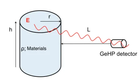
Fig. 1. Model used to build the efficiency emulator
In order to explore the capabilities of the nuclear material quantification method exposed in sections II to VI, a design of experiments related to the measurement of different more or less complex objects has been built. It concerns four gamma spectrometry experiments, so-called E1, E2, E3 and
CO. All of them consider the measurement of standard cylindrical objects used in usual processes of nuclear waste package management and contained various quantities of gamma-emitter 239
P u masses. The four objects are filled with different attenuation materials and densities. Experiment features are gathered in Tab. 1:
L(cm) h(cm) r(cm) Materials M(g) ρ(g.cm−3)
E1 117 80 30 Vinyl 0.37 0.1
E2 99 80 30 Vinyl/Metal 1.95 0.35
E3 98.5 80 30 Vinyl 0.28 0.15
CO 100 20 8 X 13 0.4
TABLE I EXPERIMENTAL DATA
In Tab. 1:
• L : Distance from detector to object (cm) • h : Cylindrical height (cm)
• r : Cylindrical radius (cm) • M : Actinide mass (g)
• ρ: Bulk density of materials (g.cm−3)
The vector X used for the construction of the detection efficiency surrogate model ǫ(X) (section IV) consists of the gamma ray energy E, the radius r and the height h of the cylinder, the distance from the detector to the object L, the density ρand the mixture of three materials: iron, vinyl, and plutonium (Fig. 1). Each of these is defined as follows in the LHS design of experiment used:
problem in considering interest data as random variables in a Bayesian framework. Section III gives some work hypothesis about interest inputs. Sections IV and V propose a method to solve the inverse problem of mass quantification and to estimate an interest mass distribution by sampling techniques. Finally, and before conclusion, sections VI and VII show quantification results, compared with experiments, in considering two different hypotheses about input uncertainties.
II. STATISTICAL APPROACH OF QUANTIFICATION
The quantification process which is considered here aims to estimate the probability density function (PDF) of an interest radionuclide mass, so-called m. Let suppose the interest radionuclide is a multi gamma-emitter. Hence, via specific software applied on gamma spectrum analysis, it is possible to obtain extracted areas from the measured gamma spectrum. Let suppose there areNextracted areas gathered in vectorS=
{S(En), n ∈ 1, N}, relatively to (En)n∈1,N energies of
the multi gamma-emitter radionuclide, andX∈ΞDrepresents a D-dimension vector of inputs for the absolute efficiency calibration coefficients vectorǫ(X)estimation. Hence, (1) and (2) allow us to provide the following equation:
S=A ǫ(E)Iγt=mAmǫ(E)Iγt
Let suppose thatYobs
is the observation vector defined in (3):
Yobs= S
IγtAm =mǫ(X) +ξ, ξ∼ N(0, σobs) (3)
In (3), ξ represents the Yobs
observation uncertainty vector. All of its coefficients are related to normal distributions centered at zero with σobs = (σobs,n)n∈1,N as standard
deviation vector. In considering Yobs
, m, ǫ(X), and X as random variables, or vectors composed by random variables, the marginal PDF for m mass given Yobs, expressed as
f(m|Yobs), is given by Bayes theorem written in terms of PDFs [1]. The probability density f(m|Yobs) depends on joint PDF f(m,Yobs) and fYobs(Y
obs
) the marginal PDF of Yobs
[7], as expressed in following equation:
f(m|Yobs) = f(m,Y
obs
)
fYobs(Yobs) ∝
f(Yobs|m)π(m) (4)
The distribution π(m) is called prior distribution [7] and based on hypothesis, experience, or subjective opinion about
mmass. To add Xdependencies lead to obtain (5):
f(m|Yobs)∝
X
f(Yobs|m)π(m|X)π(X)dX (5)
III. HYPOTHESIS
The objective is to obtain an estimation off(m|Yobs), the probability density of m mass. Let suppose some hypothesis about necessary PDFs to provide the mass distribution:
• Yobs is a vector composed by N independent random
variablesYobs
n related to normal distributions:
∀n∈1, N, Ynobs∼ N(µn(m,X), σn(m,X) 2
) (6)
withµn(m,X)andσn(m,X)respectively the mean and standard variation obtained after the propagation of all uncertainty sources.
• Let suppose there is not any correlation between m
and X, and between components of X. Hence, the
ǫ(X) efficiency does not depend on the m radionuclide mass. In this case, withXof D-dimension composed by
(Xd)d∈1,D, prior distributions can be expressed as:
π(m|X)π(X) =π(m)π(X) =π(m) D
d=1
π(Xd) (7)
• Each prior distribution provides more or less
informa-tion about its own random variable [7]. A good known variable is associated with tight normal distribution, and so, it brings information about variable behaviour. A bad known variable with no real information about, such asm
mass orρdensity of the object, is associated with uniform distribution defining on its own definition domain. This method allows us to control real knowledge about the measured object and test different hypothesis on unknown variables.
IV. MCMCSAMPLING AND SURROGATE MODELS
The calculation of themmass conditional PDFf(m|Yobs
) leads to obtain the integral ofXappearing in (5). Nevertheless, X is composed by unknown variables such as ρ object density, and to obtain directly the integral, and of course
f(m|Yobs), becomes too hard even impossible. A solution to work around the problem is to samplemmass conditional PDF in using Markov Chains Monte Carlo (MCMC) methods. The Metropolis-Hastings algorithm allows us to sample m
mass andXcomponents PDFs in using Markov Chains theory [7]. This method needs several ten thousands of calls to the simulation code which provides the absolute efficiency cali-bration coefficients vectorǫ(X). Because of the impossibility to rapidly evaluate ǫ(X) directly with the particle transport code MCNP, a Kriging surrogate model [8], [9] is proposed to emulate it. Surrogate model [9] requires a limited number of calls to the code, which are gathered in a design of experiments (DoE), in order to first accurately and quickly build an outcome of interest functionM, and finally predict new values of interest such as:
∀X∈ΞD, ǫ(X) =M(X) (8)
A well-chosen and good-known DoE building technique is the Latin Hypercube Sample one (LHS) [10]. This kind of DoE gives very interesting space filling properties by dealing with different criterion maximization such as the minimax one.
V. CALCULATION OF THEf(m|Yobs
)PROBABILITY DENSITY
The objective is to obtain m mass conditional PDF
f(m|Yobs
). Considering (5-7-8) and the given hypothesis exposed below, the calculation of f(Yobs
|m) is due and developed as expressed in the following equation:
f(Yobs|m) = N
n=1
f(Ynobs|m) = N
n=1
1
√
2πσn
e−
(µobsn −µn)2 2σ2
n
(9) where (µn)n∈1,N and (σn)n∈1,N are determined in
considering and propagating all uncertainty sources from (3). Here,(µobs
n )n∈1,Nvector represents observation inputs
com-ing from the extracted gamma spetrum. Let begin in takcom-ing (3):
Yobs= S
IγtAm =mǫ(X) +ξ, ξ∼ N(0, σobs) (10)
Due to its calculation process which uses Kriging emulation method presented below, the ǫ(X) random variable can be written as following:
ǫ(X) =µM(X) +σM(X).δσ+emodel(X).δe (11)
δσ∼ N(0,1N), δe∼ N(0, σ
2 model)
with µM(X) = (µM
n (X))n∈1,N the predictive mean
vector ofǫ(X) andσM(X) = (σM
n (X))n∈1,N its standard
deviation vector coming from the M Kriging regression surrogate model from (8). emodel(X) represents the model error. It is noted that this uncertainty is supposed to be insignificant but kept in the calculation process. Please note that uncertainties on necessary MCNP values for Kriging model construction are taken into account during its regression process. Consequently, this error doesn’t appear in (11).
Hence, (10-11) allow us to express Yobs
PDF from Yobs n PDFs:
∀n∈1, N, Ynobs∼ N(µn, σ 2 n)
µn=mµMn (X) (12)
σ2 n =m
2
(σMn (X) 2
+σ2
model) +σ 2
obs,n (13) To finish, in considering (5-7-11-12-13), them mass con-ditional PDF can be expressed as following:
f(m|Yobs)∝
X N n=1 1 √2 πσn e−
(µobsn −µn)2 2σ2
n π(m)
D
d=1
π(Xd)dX
(14)
VI. ABOUT THEξRANDOM VARIABLE
Henceforth, the aim is to considermmass PDF and sample it with MCMC methods as the Metropolis-Hastings algorithm. Nevertheless, a remaining variable has to be approached. Because of different difficulties to accurately quantify theσobs
standard deviation vector appearing in (3) and depending on the spectrum area extraction method, two hypotheses (H1and
H2) about it are tested and compared:
H1: ξ∼ N(0, σobs=αYobs), α∈[0,1] (15) H2: ξ∼ N(0, σobs=σ1N), σ∈R (16)
The first hypothesis H1 proposes to put σobs vector pro-portional to observable values (15). In the second one H2,
σobs is constant and equal to an arbitrary value σ for all N components (16).
VII. RESULTS
A. Experimental protocol
Fig. 1. Model used to build the efficiency emulator
In order to explore the capabilities of the nuclear material quantification method exposed in sections II to VI, a design of experiments related to the measurement of different more or less complex objects has been built. It concerns four gamma spectrometry experiments, so-called E1,E2, E3 and
CO. All of them consider the measurement of standard cylindrical objects used in usual processes of nuclear waste package management and contained various quantities of gamma-emitter 239
P u masses. The four objects are filled with different attenuation materials and densities. Experiment features are gathered in Tab. 1:
L(cm) h(cm) r(cm) Materials M(g) ρ(g.cm−3)
E1 117 80 30 Vinyl 0.37 0.1
E2 99 80 30 Vinyl/Metal 1.95 0.35
E3 98.5 80 30 Vinyl 0.28 0.15
CO 100 20 8 X 13 0.4
TABLE I EXPERIMENTAL DATA
In Tab. 1:
• L : Distance from detector to object (cm) • h : Cylindrical height (cm)
• r : Cylindrical radius (cm) • M : Actinide mass (g)
• ρ: Bulk density of materials (g.cm−3)
The vector X used for the construction of the detection efficiency surrogate model ǫ(X) (section IV) consists of the gamma ray energy E, the radius r and the height h of the cylinder, the distance from the detector to the object L, the density ρand the mixture of three materials: iron, vinyl, and plutonium (Fig. 1). Each of these is defined as follows in the LHS design of experiment used:
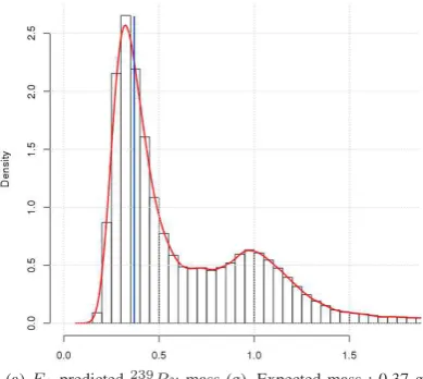
(a)E1predicted239P umass (g). Expected mass : 0.37 g (b)E3predicted239P umass (g). Expected mass : 0.28 g
(c)E2predicted239P umass (g). Expected mass : 1.95 g (d)COpredicted239P umass (g). Expected mass : 13 g
Fig. 2. Predicted239
P umasses (g) related to the four experiments underH1hypothesis withαequal to 0.05. Empirical densities appear in red and expected
masses in blue.
• h∈[10,110](cm) • L∈[80,140](cm) • ρ∈[0,1](g.cm−3)
• F e, V in, P u∈[0,100](%)
Experiments E1 and E3 represent low attenuation cases because of their respective low apparent densities and their vinyl composition. Their difference lies in the definition of the source term. The plutonium source of E1 is punctual and placed in front of the detector and in the center of the object. On the other hand, the plutonium mass of E3 is divided into 16 parts which are distributed homogeneously throughout the cylindrical object. For these two experiments, the plutonium is in the form of a liquid solution. As for them, the experiments E2 and CO are more exotic. They represent greater attenuation cases by their apparent bulk densities and their partially metallic composition. Although their respective source terms are located in a single point and therefore considered as point sources, plutonium is here in metal form and present in larger quantities. The effect of self-abortion is theoretically more expressed for these two experimental cases than for the two previous ones.
A unique characterized HPGe detector is considered for all experiments. Its characterization has been built with a numerical method developed by N. Guillot and N. Saurel [3]. The intrinsic calibration efficiency coefficient of the interest HPGe detector and its uncertainty are taken into account in the proposed quantification method. As explained in section IV, the interest conditional PDF mass f(m|Yobs
) (14) is estimated by Monte Carlo sampling in using the Metropolis-Hastings algorithm.
As explained in Section III, each parameter of the problem has itsa priori probability density. In the present case, since the radius of the cylinder, its height and the distance from detector to object are available and known, they possess a priori Gaussian probability densities centered on their real values with low variances. However, the mass of plutonium to be estimated and the bulk density possess uniform non-informative probability densities. This means that one does not have a prioriinformation on these values.
In order to propose ergodic chains [7], thirty-five Markov
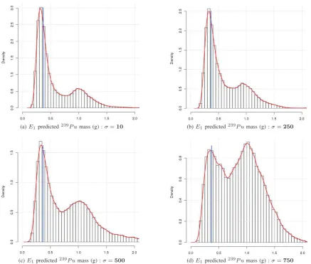
(a)E1 predicted239P umass (g) :σ=10 (b)E1 predicted239P umass (g) :σ=250
(c)E1predicted239P umass (g) :σ=500 (d)E1 predicted239P umass (g) :σ=750
Fig. 3. Predicted239
P umasses (g) related toE1experiment underH2hypothesis. Empirical densities appear in red and expected masses in blue.
chains are generated in parallel. For each of them, initial values of m mass and X input components are randomly distributed relatively to their prior distributions exposed in section III. Chain burn-ins [7] are not taken into account in mass estimated distribution analysis. Both of the H1 andH2 hypothesis presented in section VI have been tested to different values of their parameters.
B. Quantification results
For all of the four experiments, the thirty-five Markov chains are gathered to form the estimated conditional PDF mass. These distributions appear in Fig. 2 with empirical densities. For these figures, the hypothesis H1 is used with its parameter equal to 0.05,ieα= 0.05(15).
First, it is noted that the expected actinide masses of Table.1 are included in each of the distributions. With respect to the E2 and CO experiments, the mass PDFs are formed from a single distribution whose modal value is close to the magnitude of the expected mass. Gaussian, gamma and lognormal fits were attempted but without success. Moreover, the variance of the distribution of the experiment E2 is greater the CO one. As for them, the experiments E1 and
E3 propose a bimodal mass distribution. In both cases, one of the two modal values is close to the expected mass value and has greater probability amplitude. Several mixtures of fits have been tested but none showed any interesting results.
Second, the influence of hypothesesH1andH2on the form of mass distributions has been tested by varying their param-eters. Both hypotheses show similar results for the E2 and
CO experiments. Their variances increase as the uncertainty associated with H1 and H2 increases as well. Nevertheless, concerning the experiments E1 and E3, it is noted that the ratios of the probability amplitudes of their respective modals decrease as the uncertainty of the observations increases. In other words, the estimated masses from the two modals are more or less probable depending on the value of the uncertainty of the observations as shown in Fig. 3.
C. Discussion
(a)E1predicted239P umass (g). Expected mass : 0.37 g (b)E3 predicted239P umass (g). Expected mass : 0.28 g
(c)E2predicted239P umass (g). Expected mass : 1.95 g (d)COpredicted239P umass (g). Expected mass : 13 g
Fig. 2. Predicted239
P umasses (g) related to the four experiments underH1hypothesis withαequal to 0.05. Empirical densities appear in red and expected
masses in blue.
• h∈[10,110](cm) • L∈[80,140](cm) • ρ∈[0,1](g.cm−3)
• F e, V in, P u∈[0,100](%)
Experiments E1 and E3 represent low attenuation cases because of their respective low apparent densities and their vinyl composition. Their difference lies in the definition of the source term. The plutonium source of E1 is punctual and placed in front of the detector and in the center of the object. On the other hand, the plutonium mass of E3 is divided into 16 parts which are distributed homogeneously throughout the cylindrical object. For these two experiments, the plutonium is in the form of a liquid solution. As for them, the experiments E2 and CO are more exotic. They represent greater attenuation cases by their apparent bulk densities and their partially metallic composition. Although their respective source terms are located in a single point and therefore considered as point sources, plutonium is here in metal form and present in larger quantities. The effect of self-abortion is theoretically more expressed for these two experimental cases than for the two previous ones.
A unique characterized HPGe detector is considered for all experiments. Its characterization has been built with a numerical method developed by N. Guillot and N. Saurel [3]. The intrinsic calibration efficiency coefficient of the interest HPGe detector and its uncertainty are taken into account in the proposed quantification method. As explained in section IV, the interest conditional PDF massf(m|Yobs
) (14) is estimated by Monte Carlo sampling in using the Metropolis-Hastings algorithm.
As explained in Section III, each parameter of the problem has itsa priori probability density. In the present case, since the radius of the cylinder, its height and the distance from detector to object are available and known, they possess a priori Gaussian probability densities centered on their real values with low variances. However, the mass of plutonium to be estimated and the bulk density possess uniform non-informative probability densities. This means that one does not havea prioriinformation on these values.
In order to propose ergodic chains [7], thirty-five Markov
(a)E1predicted239P umass (g) :σ=10 (b)E1 predicted239P umass (g) :σ=250
(c)E1predicted239P umass (g) :σ=500 (d)E1 predicted239P umass (g) :σ=750
Fig. 3. Predicted239
P umasses (g) related toE1experiment underH2hypothesis. Empirical densities appear in red and expected masses in blue.
chains are generated in parallel. For each of them, initial values of m mass and X input components are randomly distributed relatively to their prior distributions exposed in section III. Chain burn-ins [7] are not taken into account in mass estimated distribution analysis. Both of the H1 andH2 hypothesis presented in section VI have been tested to different values of their parameters.
B. Quantification results
For all of the four experiments, the thirty-five Markov chains are gathered to form the estimated conditional PDF mass. These distributions appear in Fig. 2 with empirical densities. For these figures, the hypothesis H1 is used with its parameter equal to 0.05,ieα= 0.05(15).
First, it is noted that the expected actinide masses of Table.1 are included in each of the distributions. With respect to the E2 and CO experiments, the mass PDFs are formed from a single distribution whose modal value is close to the magnitude of the expected mass. Gaussian, gamma and lognormal fits were attempted but without success. Moreover, the variance of the distribution of the experiment E2 is greater the CO one. As for them, the experiments E1 and
E3 propose a bimodal mass distribution. In both cases, one of the two modal values is close to the expected mass value and has greater probability amplitude. Several mixtures of fits have been tested but none showed any interesting results.
Second, the influence of hypothesesH1andH2on the form of mass distributions has been tested by varying their param-eters. Both hypotheses show similar results for the E2 and
CO experiments. Their variances increase as the uncertainty associated with H1 and H2 increases as well. Nevertheless, concerning the experiments E1 and E3, it is noted that the ratios of the probability amplitudes of their respective modals decrease as the uncertainty of the observations increases. In other words, the estimated masses from the two modals are more or less probable depending on the value of the uncertainty of the observations as shown in Fig. 3.
C. Discussion
can be explained by a poor ability to predict the surrogate model M of ǫ(X)efficiency. An optimization of this model is necessary and under progress.
This method of quantification makes it possible to take into account all sources of uncertainty and to easily propagate them. Other sources of uncertainty may also be added. The optimization of the efficiency proposed above may also provide a reduction in its variance of prediction resulting from the technique of emulation by kriging.
Considering the experiment E1 under the hypothesis H2
with σ equal to 10 exposed in Fig. 3a, the variance of the estimated probability density of the mass is almost entirely due to the variance of the model of the efficiency. Indeed, given the values ofSobs
, in this case we have:
∀n∈1, N, S
obs n
σ =
Sobs n
10 ≫1 (17)
Equation (17) indicates that in the case where σ is equal to 10, it is considered to be negligible with respect to the observation. The increase in the variance visible in Fig. 3 is therefore due to the increase in the uncertainty of the observations underH2,ieσ. In caseE1, a high confidence in
the values observed, ie withσ equal to 10, makes it possible to obtain a modal approximately 6 times more likely than the second one. On the other hand, in the absence of precision on the observations, ie with sigma equal to 750, the modals estimated by the method are almost equiprobable. This case reflects the importance of accurately estimating the uncertainty of the observations, and therefore of the surfaces extracted from the gamma spectrum.
VIII. CONCLUSION
The quantification of nuclear material is essential in the nuclear industry. It allows, among other things, to comply with the legal regulations relating to the management of nuclear waste. The quantification method developed in this study uses a stochastic approach to the problem in a Bayesian framework. This makes it possible to consider all sources of uncertainty and to easily propagate them. It also proposes a resolution of the inverse problem of quantification using an MCMC algorithm. The method was tested on 4 experimental cases of 239
P u measurement. These first results are coherent and allow to glimpse a robust quantification method. The method deals with the emulation of the detection efficiency of the measurement scene. Despite good prediction capabilities, optimization of this model in terms of accuracy and variance reduction is to be expected.
REFERENCES
[1] G.F. Knoll.Radiation Detection and Measurement. John Wiley & Sons, 2010.
[2] K.Debertin and R. G. Helmer. Gamma and X-ray spectrometry with semiconductor detectors. North-Holland Amsterdam, 1988.
[3] N. Guillot. Quantification gamma de radionucl´eides par mod´elisation ´equivalente. PhD thesis, Universit Blaise Pascal, 2015.
[4] LANL. MCNP6 Users manual.
[5] A. Lyoussi. D´etection de rayonnements et instrumentation nucl´eaire. EDP Sciences, 2010.
[6] T. Vigineix. Exploitation de spectre gamma par m´ethode non param´etrique et ind´ependante da priori formul´es par lop´erateur. PhD thesis, Universit de Caen, 2011.
[7] G. Casella C. P. Robert. M´ethodes de Monte-Carlo avec R. Springer, 2011.
[8] C. E. Rassmusen. C. K. I. Williams. Gaussian processes for machine learning.MIT Press, 2006.
[9] T. Mitchell J. Sacks, W. Welch and H. Wynn. Design and analysis of computer experiments.Statistical Science, 4:409-435, 1989.