www.technology.matthey.com
Angela F. Harper*, Matthew L. Evans,
James P. Darby, Bora Karasulu,
Can P. Koçer
Department of Physics, Cavendish Laboratory, University of Cambridge, J. J. Thomson Avenue, Cambridge, CB3 0HE, UK
Joseph R. Nelson
Department of Materials Science and
Metallurgy, University of Cambridge, 27 Charles Babbage Road, Cambridge, CB3 0FS, UK; Advanced Institute for Materials Research, Tohoku University, 2-1-1 Katahira, Aoba, Sendai 980-8577, Japan
Andrew J. Morris
School of Metallurgy and Materials, University of Birmingham, Edgbaston, Birmingham, B15 2TT, UK
*Email: [email protected]
Portable electronic devices, electric vehicles and stationary energy storage applications, which encourage carbon-neutral energy alternatives, are driving demand for batteries that have concurrently higher energy densities, faster charging rates, safer operation and lower prices. These demands can no longer be met by incrementally improving existing technologies but require the discovery of new materials with exceptional properties. Experimental materials discovery is both expensive
and time consuming: before the efficacy of a new
battery material can be assessed, its synthesis and stability must be well-understood. Computational materials modelling can expedite this process
by predicting novel materials, both in stand-alone theoretical calculations and in tandem with experiments. In this review, we describe a materials discovery framework based on density functional theory (DFT) to predict the properties of electrode and solid-electrolyte materials and validate these predictions experimentally. First, we discuss crystal structure prediction using the ab initio random structure searching (AIRSS) method. Next, we describe how DFT results allow us to predict which phases form during electrode
cycling, as well as the electrode voltage profile and
maximum theoretical capacity. We go on to explain how DFT can be used to simulate experimentally measurable properties such as nuclear magnetic resonance (NMR) spectra and ionic conductivities.
We illustrate the described workflow with multiple
experimentally validated examples: materials for lithium-ion and sodium-ion anodes and lithium-ion solid electrolytes. These examples highlight the power of combining computation with experiment to advance battery materials research.
1. Introduction
The ability to store clean energy is paramount in the struggle to decarbonise the global economy; the demand for cheaper, higher performance and more sustainable energy storage technologies is growing rapidly with the market for electric vehicles and distributed energy grids. A key challenge is discovering new battery materials which outperform present technologies. However, experimental materials discovery requires extensive amounts of laboratory resources. This makes materials modelling an attractive tool that can reduce the cost and time associated with
Ab initio
Structure Prediction Methods for
Battery Materials
A review of recent computational efforts to predict the atomic level structure and
the discovery process. The effort to accurately model battery materials has been made possible largely by a quantum-mechanical theory for molecules and materials, known as DFT (1, 2). DFT is an ab initio (or first-principles) technique that requires no experimental input to make predictions about materials. By using DFT to understand how a material behaves at the atomic level, predictions can be made about its behaviour as a battery component.
Results from DFT can both guide experimental design and also help to interpret experimental results. However, in order to make these predictions, the atomic structure of the material must be known. When this is not the case, crystal structure prediction (CSP) can be used to search for the most likely arrangements of the atoms. Given a crystal structure, it is then possible to perform theoretical spectroscopy calculations, which can be compared to the experimental spectra. Examples include NMR (3), X-ray absorption spectroscopy (XAS), electron energy loss spectroscopy (EELS) (4, 5), Raman and infrared (IR) spectroscopies (6). This is especially important in the context of battery materials, as changes in the atomic structure and chemical bonding during device operation are crucial to battery function.
This review provides an overview of DFT and CSP applied to battery materials modelling and highlights recent computational research on battery anodes and solid electrolytes. Section 2 outlines DFT and CSP methods. Section 3 explains how experimentally relevant properties of battery materials can be computed. In Section 4, several examples of applying these techniques to battery materials are discussed, including conversion/ alloying anodes, solid electrolytes and anodes for Na-ion batteries.
2. First Principles Modelling of
Battery Materials
2.1 Density Functional Theory
DFT calculations have become an important part of materials research to discover and explain the causes of experimentally observed phenomena at the atomic scale. They provide insights into the physics and chemistry of materials which aid
in further optimisation of materials for a specific
application. DFT primarily provides a means for calculating the total energy and electron charge
distribution of any configuration of atoms.
The atomic-scale processes in materials are described by the quantum mechanical time-independent Schrödinger equation, Equation (i):
ĤY({Rj},{ri}) = EY({Rj},{ri}) (i)
in which the wavefunction for the set of electrons and nuclei is denoted by Ψ({Rj},{ri}) where Rj are the positions of the nuclei, ri are the positions
of the electrons and Ĥ is the Hamiltonian of the system. The energy E obtained from this equation
represents a specific energy level for the system.
In general, the ground-state energy of the system, E0, is the quantity of interest. The Hamiltonian for this time-independent equation is Equation (ii):
Ĥ = – ħ ∇j2 – ∇i2 + V({Rj},{ri}) (ii)
2 ħ2
2Mj
Σ
2mej
Σ
iThe first two terms in Ĥ are the kinetic energy operators of the nuclei and electrons, and the third is the potential energy. Nuclei and electrons interact via the Coulomb interaction. Unfortunately, the conventional Schrödinger equation is too complicated to solve beyond just a handful of particles. Therefore, approximations are required in order to solve this equation and obtain the ground-state energy of the system of interacting electrons and nuclei. Since electrons move on very fast timescales compared to nuclear motion, the
nuclei can be treated as fixed in space while the
electronic-ground state is computed. This is the Born-Oppenheimer approximation, which results in a Schrödinger equation for the electrons, in which the nuclear positions and charges enter as parameters only. The underpinning principle of DFT, the Hohenberg-Kohn theorem (1), builds from this approximation, providing a theoretical basis for working not with the wavefunction, but with the much simpler ground-state electron density, n(r).
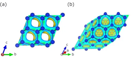
Figure 1 shows an example of the calculated ground-state electron density of the atoms in a silicon crystal structure, represented by the smooth surface surrounding the atoms. The total energy of
a system of electrons and fixed nuclei is a function
of all possible electron density functions. Using
the Kohn-Sham ansatz, finding the ground-state
electronic density is made computationally feasible by expressing it in terms of auxiliary wavefunctions
which describe a fictitious non-interacting system
of the same density (2). The full expression for the ground-state energy EKS may then be written as Equation (iii):
EKS = T[n] + ENN + d3rVext(r)n(r) (iii)
+ d3 rd3r' + E
XC
1 n(r)n(r') 2 |
∫
r – r'|where the first term, T n , is the kinetic energy associated with the non-interacting Kohn-Sham particles; the second term, ENN, is the nuclear-nuclear interaction; and the third term, Vext, is the external potential of ion cores in which the
electrons move. The fourth and fifth terms
represent electron-electron interaction energies. The fourth term is the exact classical electrostatic energy; the interaction energy of an electron with
the mean field of all electrons. The fifth term is
the exchange-correlation energy, which attempts to account for all interactions not accounted for
within the first four terms. By dividing up the
energy in this way, while the exact exchange-correlation functional remains unknown, it may be approximated in various tractable ways.
The simplest approximation to EXC is the local density approximation (LDA), where the exchange-correlation energy per particle is taken to be equal to that of a uniform electron gas of the same electron density, at each point in space. Generalised gradient approximation (GGA) functionals improve on the LDA by taking into account both the electron density and the gradient of that density, resulting in a more accurate description of exchange and correlation (3). These functionals have limitations; most seriously, both electron localisation and electronic band gaps are underestimated. So-called ‘hybrid functionals’ have aimed at semi-empirically correcting the electronic band gap (4) and developing functionals beyond the LDA and
GGA is the focus of much of the theoretical work
in the field of DFT today, where the ultimate goal is to find an exchange-correlation functional which
accurately describes all possible systems (5). Within this framework, total energies, forces, equilibrium geometries, elastic behaviour and many other properties of interest can be readily and accurately predicted. However, to predict a material’s properties using DFT, it is necessary to know how its atoms are arranged. Thus, in the following section, we describe the method of CSP, which uses DFT to generate structures of novel materials.
2.2 Crystal Structure Prediction
There are multiple materials databases. Some contain only the experimental crystal structures and other relevant properties of known materials, while others contain the computed properties of both known and hypothetical materials. These can be leveraged to perform CSP. For example, known crystal structure prototypes can be decorated with any set of atomic species, resulting in new hypothetical materials. The stability and synthesisability of these new materials can then be assessed using DFT calculations and by comparing against thermochemical data in the database. Three of the major exhaustive databases of DFT calculations, the Open Quantum Materials Database (OQMD) (6), the Automatic Flow (AFLOW) framework for materials discovery (7) and the Materials Project (8) have been used to predict new materials and screen for desired properties using a combination of high-throughput ab initio calculations and, increasingly, statistical and machine learning approaches. In addition,
experimentally identified structures are found
in the Inorganic Crystal Structure Database (ICSD) (9) and the Crystallography Open Database (COD) (10). These databases have been used as a starting point for many theoretical studies,
leading to several new discoveries in the field of
energy storage, including identifying SrFeO3-δ as a material for carbon capture (11), verifying Li3OCl as a solid electrolyte with high ion conductivity (12) and predicting LiMnBO3 as a Li-ion battery cathode (13). While these databases are useful for comparisons of known structures and enable the discovery of materials that are based on known crystal structure prototypes, it is likely that new
structures exist which cannot be classified as one
of the currently known prototypes. Therefore, it is necessary to perform CSP in order to explore novel phases of materials.
(a) (b)
c
a b
c a b
The search for new thermodynamically stable materials (those favoured to form during synthesis, when kinetic factors are excluded) using CSP can take one of many approaches (14), but all involve a search for the lowest energy minimum
in a high-dimensional configuration space. The configuration space for a periodic structure with
N atoms per unit cell has dimension 3N+3, taking into consideration the rotational symmetries and unit-cell degrees of freedom, whilst the number of local minima in the space scales exponentially with N (15). Ideally, all low-lying minima would be sampled during CSP since metastable phases may be synthesised experimentally, or indeed
be thermodynamically stable under different
conditions; for example, graphite is the most stable allotrope of carbon under ambient conditions, but diamond can be easily synthesised under high pressure. Particularly popular approaches to CSP include the use of evolutionary algorithms to ‘breed’ new structures (15) and particle swarm optimisation (16–18).
AIRSS (19) is the focus of this review. Despite the potential for having a high computational
cost, AIRSS remains an effective method for
structure prediction which allows for a breadth of searching and has proven successful in a wide range of materials. Beyond the ease of its implementation, AIRSS has several advantages. Firstly, individual relaxations do not depend on one another, hence all trials can be run concurrently making the algorithm trivially parallelisable to the largest of supercomputers. Secondly, AIRSS allows for the easy application of chemically
intuitive constraints which reduce the initial search space to the most experimentally relevant trial structures. This constraint greatly reduces the size of the search space and makes AIRSS applicable to a wide range of systems, including those at high pressure (20, 21). These chemical constraints include, for example: the phases of conversion and alloying anodes (22–25) were constrained by space group symmetries and atomic distances; high pressure phases of ice (26) were constrained to H2O units; encapsulated nanowires (27) were constrained by rod group symmetries; metal-organic frameworks (28) were constrained to molecular building blocks; grain-boundary interfaces (29) and point-defects (30)
had some atoms fixed to describe the lattice
and systematically randomised other atoms to describe interface and defect structures.
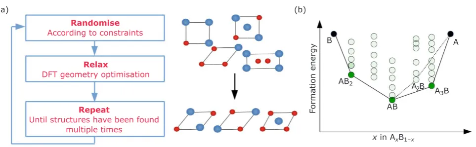
AIRSS explores configuration space using random
sampling as shown in Figure 2(a) and proceeds as follows.
To search for a new phase with chemical formula, AxBy, any number of atoms of element A and B
are placed randomly (denoted ‘Randomise’ in Figure 2(a)) into a 3D simulation cell in the ratio x:y. The cell and atomic positions are allocated such that they obey a set of chosen symmetry operations (a space group in 3D). Further constraints, such as minimum separation between atoms and a feasible range for the atomic density of the unit cell, may be imposed. These constraints narrow the region
of the configuration space of possible structures
by avoiding regions that describe unrealistic arrangements of atoms.
(a) (b) Randomise
According to constraints
Relax
DFT geometry optimisation
Repeat
Until structures have been found multiple times
Formation energy
x in AxB1–x B
AB2 A
2B A
3B AB
A
Fig. 2. (a) Workflow schematic of the AIRSS method which is used to find the ground-state structures of different materials; (b) example of a convex hull of elements A–B which details how AIRSS can identify a
The forces on the atoms and stresses on the cell are calculated with DFT and then minimised using the traditional optimisation algorithms (for example, conjugate gradients). This step is denoted ‘Relax’ in Figure 2(a). The energy of the system is used as a metric to gauge how stable the structure is.
Steps 1 and 2 are then repeated several thousand times in order to generate a representative set of structures in the A-B chemical space. The search is stopped once the lowest energy structures have been found multiple times. The set of lowest energy structures are the candidates for phases that are likely to form experimentally.
Using the DFT energies, one can construct a ‘convex hull’ of all the structures found by AIRSS, as shown in Figure 2(b). The structures AxBy
which are likely to form, must both have a negative formation energy relative to elemental A and B and lie on the convex hull tie-line between A and B to avoid decomposition into other binary phases. This tie-line is shown by the black line connecting the lowest energy structures in Figure 2(b). This
figure illustrates the process of constructing a
convex hull using the optimised structures from AIRSS. Suppose at a given point during the AIRSS search, the only structures on the convex hull are AB, AB2 and A2B, connected by the dashed line in Figure 2(b). Subsequently, a novel phase, A3B, is identified using AIRSS and is found to lie below the existing tie-line. In this case, CSP has
identified a new ground-state structure which
suggests an additional phase, A3B is likely to exist within the A-B phase diagram. Therefore, as shown in Figure 2(b), the hull is reconstructed to include the phase A3B, rendering A2B unstable, given that it is now no longer on the convex hull. Although this example is given for two dimensions (i.e. a binary system containing elements A and B) the convex hull construction is generalisable to N dimensions, in which the tie-lines between the lowest energy structures are computed in a similar manner.
In this way, AIRSS enables the prediction of new thermodynamically stable and metastable compounds in a given phase diagram and the convex hull construction provides a guide to their stability compared to previously known phases, without performing exhaustive chemical synthesis. Synthesis experiments can then be targeted at the most promising compositions and characterisation experiments can be guided by the predicted model structures.
3. Calculating Experimentally
Observable Properties
Once a structure is obtained, either through CSP or from a database, it is possible to use DFT to calculate many experimentally observable properties. In this section, we highlight several methods for calculating quantities which are experimentally
relevant to the field of battery research, especially
regarding electrodes and solid electrolytes.
3.1 Theoretical Voltage Profiles
The electrochemical voltage profile is the voltage
signal of the electrode measured (vs. a reference, usually Li+/Li) as a function of the number of ions (i.e. charge) stored in the electrode. The phase transitions, which occur within the electrode during cycling provide the characteristic shape of the
voltage profile; two-phase regions show a constant
voltage, while solid-solution regions show a sloping voltage. The voltage drop between two phases is
proportional to the difference in their free energies
and thus these voltage drops can be computed directly from the free energies of the phases which lie on the convex hull tie-line. The voltage-drop between two phases with active ion concentrations x1 and x2 is Equation (iv):
V = –qDGrxn (iv)
(x2 – x1)F
where q is the charge of the active ion, F is the
Faraday constant and ∆Grxn is the change in Gibbs free energy between phases. In practice, the change in Gibbs free energy in Equation (iv) is approximated by the change in the DFT total energy, under the assumption that entropic
contributions will have a minimal effect on the free energy differences between phases during cycling.
When studying a phase diagram computationally
there are a finite number of phases on the tie-line, thus the profile will not be a continuous smooth
line, but a sequence of two-phase regions with
constant average voltages. Although the profile
will not have the same characteristic curve as an
experimental voltage profile, it is still possible to
calculate quantities of interest such as theoretical capacity, which is calculated from the maximal
difference in active ion concentration between
the predicted stable phases. Similarly, the energy density of an electrode is found by integrating the
3.2 Computational Nuclear Magnetic
Resonance Spectroscopy
Beyond calculating the voltage profile, one may
further validate a crystal structure against experiment by using DFT to predict its spectroscopic signatures. Many spectroscopic methods, including XAS, EELS (31) and Raman spectroscopy (32), can be readily calculated using DFT to aid characterisation.
Solid-state nuclear magnetic resonance (ssNMR) spectroscopy is a tool for investigating the
element-specific local structure of materials, even for the
disordered and dynamic systems present in battery materials (33). Due to the complex structures and processes that arise during battery cycling, the usefulness of NMR spectroscopy can be greatly enhanced by applying complementary techniques to aid the assignment of spectra to the local environment of each nucleus. Theoretical methods
in DFT are sufficiently mature that the calculation
of chemical shielding tensors across a diverse range of inorganic systems is now routine (34).
NMR spectroscopy involves the precise measurement of the response of nuclei in an applied
magnetic field to weak oscillating perturbations; for
a given pulse scheme, the frequency of perturbing oscillations is adjusted until resonance is achieved, at which point a signal is observed. The frequency of this resonance is a cumulative measure of several competing interactions between the spin of
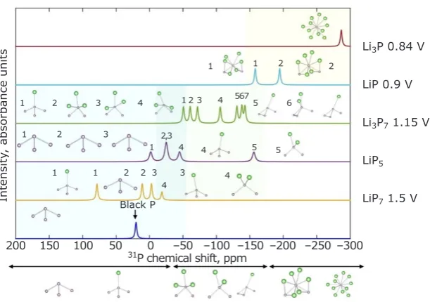
the nucleus and its local environment and, when referenced against a model nucleus, is referred to as the chemical shift. The observed chemical shift in most materials is determined by the nuclear spin interacting with the orbital angular momentum of paired electrons. In Figure 3, such a shift is given for the phases of Li-P which form during cycling of a Li-ion battery with a phosphorus anode (22). The 31P chemical shift of each Li
xPy
phase is distinct, as shown by the coloured peaks
in the figure for each compound.
Whilst the theory for computing magnetic shielding for isolated systems (such as molecules and clusters) was developed in the 1960s and 1970s in the context of quantum chemistry (35), these methods were not easily extendable to solids (36). For periodic systems, such as battery anodes and cathodes, most modern implementations of theoretical ssNMR use DFT and the gauge including projector augmented wave (GIPAW) approach (37–39). It is not only possible to compute the full chemical shielding
tensor, but also several other effects that can
modify the lineshape of the NMR signal, namely quadrupolar coupling (for spin I��>1 2/ nuclei), dipolar coupling (which can be simulated directly from the geometry using for example the SIMPSON software package (40)) and J-coupling (interaction of electron spins which can probe chemical bonds directly) (41).
Fig. 3. Calculated 31P NMR chemical shifts (22) for various thermodynamically stable Li-P compounds found using a combination of data mining and AIRSS. The shifts show a clear trend towards more negative shifts (increased chemical shielding) as the Li content of the structures increases. This is related to the number of nearest neighbour Li ions of each P. These DFT predictions of NMR shifts enable experimentalists to correlate
observed shifts with specific local structure environments. Reproduced with permission from the American
Chemical Society
Li3P 0.84 V
LiP 0.9 V
Li3P7 1.15 V
LiP5
LiP7 1.5 V
Intensit
y, absorbance units
1 1 2 2
1 2 3 4 1 2 3 4 567 5 6
1 2 3 2,3
1 4 4 5 5
1 1 2 2 3 4
3 4
Black P
3.3 Predicting Transport Properties
with DFT
Finally, beyond just characterising the static crystal structure of a battery material, it is also possible to predict the dynamics of ions moving through the material, which is especially useful when studying ionic transport in electrodes and solid electrolytes. The charge and discharge rates are
key performance factors in battery design, defining
the time required to fully charge a battery and the amount of power it can deliver, respectively. Rate capability is determined by the speed with which the charge carriers can move through the materials. Since both ions and electrons move in a battery, the rate capability depends on both the electronic and ionic conductivity of the materials. While the electrodes in batteries must be mixed electronic-ionic conductors, the electrolyte must be electronically insulating. First principles methods, such as DFT, can be used to study both electronic conductivity and ionic conductivity of battery materials. Electronic conductivity can be assessed from electronic structure calculations (42–44), while ionic conductivity can be calculated using ab initio molecular dynamics (AIMD) or the nudged elastic band (NEB) method (45), as outlined below.
The bulk ionic conductivity, σ( )T , of a solid
electrolyte can be related to diffusion coefficients
via the Nernst-Einstein relation (46) defined as
Equation (v):
s(T) = ne2z2D(T)HR (v) kBT
where n is the diffusing particle density, e the elementary electron charge, z the ionic charge, kB the Boltzmann constant, T the temperature, D T
( )
the ionic diffusivity and HR the Haven ratio accounting for the correlated ionic motion.3.3.1
Ab Initio
Molecular Dynamics
Simulations
One way to compute ionic diffusivity of a given
material, using AIMD simulations, combines the
first principles aspects of DFT with the ability of
molecular dynamics (MD) to model ionic forces and trajectories. Methods to screen the mobility of ions along an MD trajectory include mean square displacement (MSD), mean jump rate (MJR) (47, 48), velocity autocorrelation function (VACF) (49– 52) van Hove correlation function (53, 54) and others (55, 56). MSD is the most straightforward
and robust and thus the commonly used definition of diffusivity.
One can extract the diffusion coefficient D T
( )
from the gradient of the MSD, given a well-converged MD trajectory such that the MSD is a linear function of time. Here, the slope of theline of best fit gives the diffusion coefficient D, times twice the dimensionality d of the diffusion
(2d D* ). For ionic diffusion in three dimensions,
d =3. Depending on the level of mobility of ions in the system, good convergence of the MSD of ions may require long trajectories, for example 50–100 ps, thereby requiring tens of thousands of time steps. As each step involves DFT energy or force evaluations, AIMD can be a computationally demanding process. Two common solutions to this are: (a) to analyse trajectories obtained at elevated temperatures (500–2000 K) to foster higher mobility and faster convergence of the MSD; or (b) to utilise parameterised atomic
force-fields to allow faster evaluation of the interatomic
forces in the system compared to ab initio methods
like DFT. A drawback of parameterised force-fields
is non-transferability, so one needs a new set of
fitted parameters for the specific set of atoms in a
new system.
The activation energy (Ea) for the ionic transport in a given electrolyte or electrode can be obtained from AIMD simulations using the Arrhenius law, Equation (vi):
D(T) ≈ D0e–Ea/kBT (vi) where D0 is the theoretical maximum diffusivity at infinite temperature, under the assumption that the diffusion mechanism is not temperature dependent
and no phase transition occurs. Analysis of the trajectories from the AIMD simulations can also provide useful information on the crystallographic sites with higher occupation probability, while also revealing the preferred ionic conduction pathways between these sites (47, 57, 58).
3.3.2 Nudged Elastic Band Method
Another way to obtain ionic diffusivity from firstprinciples is with optimisation-based methods, through the exploration of minimum energy
paths (MEP) describing a set of predefined ionic
migration pathways. To this end, the NEB algorithm is often used. Other approaches are also available for transition-state searches, for example the dimer (59), Lanczos (60) and eigenvector-following (EF) (61) methods as well as others (62, 63).
0 K) for a predefined route connecting the initial and final states of the motion of a single ion or a few, concertedly diffusing ions (45, 64). The
ion-transport path is divided into intermediate steps
(called NEB images), defined by the interpolation
of these two end-point states. The NEB images are concurrently optimised by introducing a set of imaginary spring-forces to ensure the harmonic coupling of the consecutive images and a continuous path on the corresponding high-dimensional potential energy surface. Using the climbing-image NEB that maximises the energy of the saddle point(s) on the MEP, one can also locate the transition states, from which activation energies (Ea) are calculated.
In solids, the change of entropy during ionic
diffusion is usually negligible and thus activation
free energies are typically approximated by their
0 K values. The diffusion rate can then be related to the ionic diffusivity in the dilute carrier limit (65) (i.e. diffusion carriers do not interact) using
Equation (vii):
D = l2gfx
Dν*exp – DkEa (vii)
BT
where� �λis the hop distance between two adjacent sites, g is a geometric factor that depends on the symmetry of the sublattice of interstitial sites, f is the correlation factor, xD is the concentration
of the diffusion-mediating defects, v* is the
entropy difference between the initial and final
states, the activation energy Ea is the energy
difference between the initial and final states, kB is Boltzmann’s constant and T is the temperature of the simulation.
Static methods, such as NEB, provide
computational efficiency over AIMD: NEB requires
only a few hundred DFT steps to converge and is accurate within the regime in which the electronic structure of the model system does not change with the ionic migration (66). NEB calculations also allow
for quantitative comparison of different migration
routes. Nevertheless, NEB is less likely to reveal new conduction mechanisms compared to AIMD, and the complex cooperative conduction mechanisms may not be as straightforward to sample with NEB as with AIMD. Moreover, NEB usually operates in the dilute regime (Equation (vii)), where vacancy defects are manually introduced in the sublattice
of the diffusing ions to have a low diffusion carrier
concentration and mediate the ionic motion. These
artificial defects not only decrease the accuracy
of the simulation models, but also impede the integration of the NEB method in high throughput
approaches. AIMD, in contrast, would in principle
work with any concentration of diffusing ions by readily addressing the self-diffusion limit (67, 68). Given these tradeoffs, a common practice in
the literature is therefore to combine AIMD with
NEB calculations, specifically by identifying the
potential conduction pathways from relatively shorter AIMD trajectories at a selected, elevated temperature and to probe the MEPs to get Ea and compute the other properties relevant to the ionic transport (57, 58, 69–71).
In many cases, as in the voltage high-capacity anode material TiNb2O7 (TNO), both ionic and electronic conductivities are relevant to the performance of the battery material (72). In this case, density of states (DOS) calculations were used to determine that the electron-doped TNO is metallic, as compared to the pristine TNO. Additional localised electronic states were
confirmed in AIMD as a result of bond distortions,
thus exemplifying the need in this case for both AIMD and DOS calculations.
4. Applications to Modelling
Rechargeable Batteries
Each of the theoretical methods described in Section 3 still require a model crystal structure which can be obtained either from CSP or
experiments. Thus, we establish a workflow
from prediction to realisation in several simple
steps. The general outline of this workflow is
to: (a) use AIRSS or another CSP method to search for novel phases; (b) characterise these materials using DFT; (c) use DFT to predict and compare to experimental spectroscopy,
or AIMD and NEB to predict diffusion pathways
through ionically conducting materials. Large computational databases can be constructed for a particular electrode material, where one phase diagram may contain as many calculations as the entire databases mentioned in Section 2.2; the Python package ‘matador’ (73) has been created
to perform this high-throughput workflow and
automate this database construction from CSP results. The following sections provide examples
in which this workflow has been successfully
usually be enumerated and the most probable
configurations studied using a cluster expansion
(66, 74, 75).
4.1 Modelling Conversion and
Alloying Anodes for Lithium-ion
Batteries
Graphite is ubiquitous in contemporary commercial Li-ion batteries. However, alternative anode materials are a highly researched topic, due to graphite’s low capacity (372 mAh g–1) and tendency for Li plating and subsequent dangerous short-circuiting due to its low operating voltage (76). These factors make graphite anodes unattractive for applications that require high performance and capacity, such as electric vehicles.
Here we highlight developments in predicting high capacity conversion and alloying anodes to replace graphite, based on tin (990 mAh g–1) and antimony (660 mAh g–1). Such conversion and alloying anodes undergo a succession of reversible phase transformations during charging and results in their observed higher capacity retention than other conversion and alloying anodes (77).
Both Sn and Sb were previously employed as anodes in Li-ion batteries, showing evidence of conversion reactions, with unknown phases of LixSn
and LixSb forming during Li insertion. An AIRSS
search for the thermodynamically stable phases of both LixSn and LixSb was conducted (23, 78)
in order to understand the voltage profiles and
reaction mechanisms of these two alloying anodes. In this case, a new phase Li2Sn was identified by AIRSS to lie near the convex hull. The resulting
voltage profile is compared with experimental
measurements in Figure 4.
During the cycling process in conversion anodes such as Sn, the material at the anode undergoes several conversion reactions as Li is inserted (77).
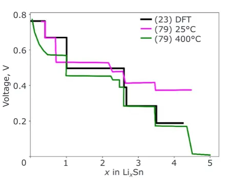
In the voltage profile shown in Figure 4, the black line is constructed from the ground state phases in the Li-Sn system, which were predicted using AIRSS (23, 78). Each plateau in Figure 4 represents a two-phase region between one ground state Li-Sn alloy and another, until a critical point is reached at which there is a phase transformation (a vertical line) to the next Li-Sn alloy.
The DFT predictions lie within the voltage range of the experiment and are an accurate match to both sets of experimental data by Wang et al. (79). In many cases, the experimental data has less-sharp distinctions between separated phases, due to reactions which appear to occur gradually rather
than at a well-defined stoichiometry.
The Li-Sb phase diagram was found to be somewhat simpler, with only two stable phases predicted during cycling: Li2Sb and Li3Sb. Two competing polymorphs of Li3Sb were found and NMR calculations were performed on both to provide a signature of each phase to aid the interpretation of future experiments.
This work on Li-Sn and Li-Sb anodes provided
theoretical confirmation of experimental binary
phases in this family of conversion anodes and
allowed for more concrete evidence of the specific
mechanism of Li insertion into these anodes.
Furthermore, this study confirmed the new phase
of Li2Sn.
4.2 Modelling Lithium Diffusion in
Solid Electrolytes
The electrolyte in a battery forms a conductive bridge between the anode and cathode which allows ions to move from one electrode to the
other without permitting the flow of electrons.
Conventional Li-ion battery architectures use a liquid electrolyte consisting of a Li salt mixture dissolved in an organic solvent. Two prominent safety concerns arise from the use of organic
liquid electrolytes (80, 81). The first is that the organic solvent component tends to be flammable and poses a fire hazard when exposed to air if the
battery casing is breached (82). The second is that Li dendrites (83, 84) form, which can eventually bridge the gap between the anode and cathode resulting in short-circuiting.
Fig. 4.Comparison between theoretical and
experimental voltage profiles for the Li-Sn
conversion anode. The black line is the theoretical
predicted voltage profile based on the phases that
are on the convex hull tie-line (23), which matches well with the experimental results of Wang et al., shown in magenta and green for 25°C and 400°C respectively (79)
(23) DFT (79) 25°C (79) 400°C
Voltage, V
1 2 3 4 5 x in LixSn
0.8
0.6
0.4
0.2
All solid-state batteries attempt to solve these safety issues by replacing the organic electrolyte solutions with solid equivalents, which exhibit high mechanical strength, suppressing dendrite formation, thus enabling the use of the high energy density Li-metal anodes (85, 86). Most proposed
solid electrolytes have sufficient mechanical
strength, as demonstrated by high throughput screening based on machine learning methods (87).
A key challenge in developing solid electrolytes
is finding solids with room temperature (RT) ionic
conductivities that approach those of their liquid counterparts. Among several solid electrolyte
families identified to date, the thiophosphide
ceramics, for example Li2S-P2S5,
chemically-doped sulfides, like Li10GeP2S12 (LGPS) (88) and Li9.54Si1.74P1.44S11.7Cl0.3 (89), are known to deliver the highest RT Li-ion conductivities (1.2– 2.5 × 10⁻² S cm–1). Sulfides, however, have high moisture sensitivity and their chemical stability against common electrodes is low, thus limiting their practical use (90). By contrast, oxides like garnets (for example, LixLa3M2O12, where M = zirconium, niobium, tantalum) display notably
higher chemical stability than sulfides but exhibit
lower ionic conductivities (91). The latter limitation can be partly remedied by a chemical doping with diverse metals, including aluminium, gallium and scandium (92).
High throughput CSP is useful for exploring new superior electrolytes with combined high conductivity and chemical stability. Various studies have performed extensive screening of superionic conductors within databases such as the Materials Project (8), searching for phases with good phase stability, high Li+ conductivity, wide band gap and good electrochemical stability (12, 53, 93–95).
Various LGPS-derived compositions were predicted using ab initio calculations through elemental swapping (95), such as Li10(Sn/Si)PS12
and then verified by experimental synthesis and
measurements (96, 97). LiAlSO was discovered solely through structure prediction and proposed to be a superionic conductor with AlS2O2 layers, which facilitate faster movement of Li-ions, low activation barriers and a wider electrochemical window (94). Similarly, Fujimura et al. (98) presented a high throughput (HT) screening of the chemical phase space for Li3.5Zn0.25GeO4 (LISICON)-type electrolytes. The authors proposed new electrolytes with higher conductivities than the parent LISICON material. Later, Zhu et al. (93) reported a HT screening of the Li-P-S ternary and Li-M-P-S (where M is a non-redox-active element)
quaternary chemical spaces and identified two Li
superionic conductors, Li3Y(PS4)2 and Li5PS4Cl2. Particularly, Li3Y(PS4)2 is predicted to exhibit a room-temperature Li+ conductivity of 2.16 mS cm–1, which can be further enhanced with aliovalent doping (93). However, these materials are yet to be synthesised.
Following the structure prediction of these new solid electrolyte phases, it is then desirable to use NEB and AIMD simulations to investigate the atomistic origins of their ionic conductivity. For instance, Li-ion transport was elucidated in the
sulfide-based electrolytes, Li7P3S11 (99), argyrodite Li6PS5Cl (48, 53), LGPS (57, 100), Li-Sn-S/Li-Sn- Se (101, 102) and Li-As-S/Li-As-Se alloys (103), Li3PS4 (48, 104, 105), Li4GeS4 (57, 103) as well as oxides, for example LLZO (71, 106–108), LiTaSiO5, LiAlSiO4 (71), Li4SiO4−Li3PO4 solid mixtures (109) and several others. The problem of identifying solid electrolyte candidates for all solid-state batteries which are air stable and highly conducting can be solved using a combination of structure prediction techniques and atomistic modelling such as AIMD and NEB.
4.3 Beyond Lithium: Applying
Structure Prediction to Na-ion
Batteries
So far, the battery materials we have discussed (Sections 4.1 and 4.2) are based on Li-ion chemistry. However, cost and sustainability
are driving research efforts into ‘beyond Li-ion’
batteries. The philosophy presented in Section 3, using CSP and DFT, is straightforward to extend to ‘beyond Li-ion’ chemistries. A prominent example is Na-ion batteries, where Li is replaced with the more earth-abundant Na.
Unlike in Li-ion batteries, graphite shows poor capacity for Na, although other carbonaceous
materials offer some promise (110). As such,
so its cycling is expected to involve multiple phase transformations. For these reasons, there has been recent focus on understanding sodiation processes in P.
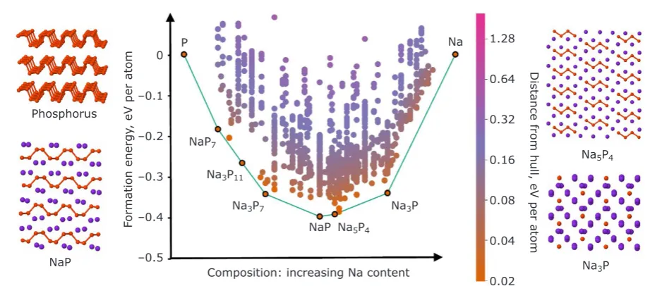
Applying a combination of AIRSS, data mining (22) and a genetic algorithm (25), the convex hull of the Na-P system has been mapped out and is shown in Figure 5. The Na-P system contains a number of stable crystalline phases (coloured black circles in Figure 5) with compositions varying from NaP7 through Na3P, and the voltage curve derived from these phases shows good agreement with experimental measurements (25). In addition to these stable phases, there are metastable phases lying close to the convex hull across a range of compositions.
By following the structures which fall on or near the convex hull in Figure 5, from least sodiated (pure P) to most sodiated (Na3P), the calculations predicted many changes in local structure: the layered black P is broken upon successive Na insertion, forming P chains and helices, then dumbbells, which eventually break apart to form isolated P atoms. These structural motifs are distinctive and have characteristic NMR signatures, which can be accurately modelled. In order to
confirm this explicitly, ex situ 31P solid-state NMR
measurements were taken at different points during
both the sodiation and desodiation cycle (25). Since
contemporary NMR calculations lack a rigorous treatment of paramagnetic contributions to the isotropic shifts, the chemical shift anisotropies were computed for the thermodynamically accessible range of predicted structures to provide a set of chemical environments to screen against experimental measurements. During the reverse cycle when Na is removed from the system, P helices re-formed in a tangled fashion and the original crystalline P was not recovered. Amorphous phases were encountered experimentally on desodiation and, while modelling of amorphous materials is challenging, the local structural features of predicted metastable phases were discovered to be present even in the amorphous structures.
Aside from P, Sn also shows promise as a Na- ion battery anode. Sn presents a lower theoretical capacity for Na (847 mAh g–1) but offers better capacity retention than P (24). The results of an AIRSS search for Na-Sn phases (24), predicted that insertion of Na into Sn would result in hexagonally layered structures NaSn3 and NaSn2, before passing through an amorphous phase of approximate composition Na1.2Sn, after which a solid-solution consisting of Sn dumbbells surrounded by Na
ions would form. The final product, Na15Sn4, contains isolated Sn atoms surrounded by Na.
Importantly, the computational workflow used to
study Li and Na-ion batteries is the same and
Fig. 5.Convex hull (see Figure 1(b)) of the Na-P system as predicted using DFT through a combined approach using data mining, AIRSS and an evolutionary algorithm (22, 25). The ground state phases are
labelled below the green tie line and their chemical compositions are given. The inset figures around the
convex hull show the structures of intermediate Na phosphides, which are related to the structure of black P shown in the top left corner. In these structures the orange spheres represent P atoms and the purple spheres represent Na
Phosphorus
NaP
Formation energy
, eV per atom
0
–0.1
–0.2
–0.3
–0.4
–0.5
Composition: increasing Na content P
NaP7
Na3P11
Na3P7 Na3P Na5P4
NaP
Na 1.28
0.64
0.32
0.16
0.08
0.04
0.02
Distance from hull, eV per atom
Na5P4
is equally as applicable to conversion anodes for other chemistries.
5. Conclusion
In this review, we have provided an overview of computational modelling of battery materials using DFT, with a focus on cases where the atomic structure of the material is unknown. In these
cases, CSP methods are used to find the most
stable arrangements of the atoms during battery operation. Once the atomic structure is known, a variety of theoretical spectroscopy and other modelling techniques can be employed to compare these computational results to experiments. These include the prediction of NMR spectra, the probing of ionic conductivities using the AIMD or the nudged elastic band method and the construction
of voltage profiles. In this way, CSP combined
with chemical synthesis can accelerate battery research by creating a feedback loop between experimentalists and theorists. One method for CSP, AIRSS, has been used as a tool to predict new phases in battery electrodes and has been shown
to be effective both for understanding the atomistic
mechanisms for electrodes and electrolytes which are already in use, and for discovering new chemistries beyond those used in contemporary Li-ion batteries.
By reducing the experimental trial-and-error necessary to optimise new battery chemistries, computational modelling has the potential to reduce the time-to-market for novel device chemistries, as well as providing overarching design principles. In addition, CSP, and atomistic modelling more generally, can now be used to screen for new battery chemistries within the application-imposed constraints on performance and sustainability, with the goal of circumventing the need for unsustainable materials such as cobalt. This growing interplay between modelling and experiment will be crucial to meeting energy storage goals required for decarbonisation.
Acknowledgements
Angela Harper acknowledges the financial support
of the Gates Cambridge Trust, University of Cambridge, UK. Matthew Evans acknowledges the Engineering and Physical Sciences Research Council (EPSRC) Centre for Doctoral Training in Computational Methods for Materials Science, UK, for funding (EP/L015552/1). Can Koçer would like to
thank the EPSRC for financial support. Angela Harper
and Can Koçer acknowledge the Winton Programme for the Physics of Sustainability, University of Cambridge, UK. James Darby acknowledges the funding provided by the Sims Fund, University of Cambridge, UK and EPSRC. Andrew Morris and Bora Karasulu would like to acknowledge funding from EPSRC (EP/P003532/1). The authors acknowledge networking support via the EPSRC Collaborative Computational Projects on the Electronic Structure of Condensed Matter (CCP9) (EP/M022595/1) and NMR crystallography (EP/M022501/1). Computing resources on the Tier 1 resource ARCHER were provided through the UKCP EPSRC High-End computational consortium (EP/P022561/1) and on the Tier 2 resources HPC Midlands+ (EP/P020232/1) and CSD3 (EP/P020259/1).
References
1. P. Hohenberg and W. Kohn, Phys. Rev., 1964,
136, (3B), B864
2. L. J. Sham and W. Kohn, Phys. Rev., 1966,
145, (2), 561
3. J. P. Perdew, K. Burke and M. Ernzerhof, Phys. Rev. Lett., 1996, 77, (18), 3865
4. P. J. Stephens, F. J. Devlin, C. F. N. Chabalowski and M. J. Frisch, J. Phys. Chem., 1994, 98, (45), 11623
5. N. Mardirossian and M. Head-Gordon, Mol. Phys., 2017, 115, (19), 2315
6. S. Kirklin, J. E. Saal, B. Meredig, A. Thompson, J. W. Doak, M. Aykol, S. Rühl and C. Wolverton,
npj Comput. Mater., 2015, 1, 15010
7. S. Curtarolo, W. Setyawan, G. L. W. Hart, M. Jahnatek, R. V Chepulskii, R. H. Taylor, S. Wang, J. Xue, K. Yang, O. Levy, M. J. Mehl, H. T. Stokes, D. O. Demchenko and D. Morgan,
Comput. Mater. Sci., 2012, 58, 218
8. A. Jain, S. P. Ong, G. Hautier, W. Chen, W. D. Richards, S. Dacek, S. Cholia, D. Gunter, D. Skinner, G. Ceder and K. A. Persson, APL Mater., 2013, 1, (1), 011002
9. M. Hellenbrandt, Crystallogr. Rev., 2004,
10, (1), 17
10. S. Gražulis, A. Daškevič, A. Merkys, D. Chateigner,
L. Lutterotti, M. Quirós, N. R. Serebryanaya, P. Moeck, R. T. Downs and A. Le Bail, Nucleic Acids Res., 2012, 40, (D1), D420
11. C. Y. Lau, M. T. Dunstan, W. Hu, C. P. Grey and S. A. Scott, Energy Environ. Sci., 2017, 10, (3), 818
13. J. C. Kim, X. Li, C. J. Moore, S.-H. Bo, P. G. Khalifah, C. P. Grey and G. Ceder, Chem. Mater., 2014, 26, (14), 4200
14. R. Oganov, C. J. Pickard, Q. Zhu and R. J. Needs,
Nat. Rev. Mater., 2019, 4, (5), 331
15. C. W. Glass, A. R. Oganov and N. Hansen,
Comput. Phys. Commun., 2006, 175, (11–12), 713
16. Y. Wang, J. Lv, L. Zhu and Y. Ma, Phys. Rev. B, 2010, 82, (9), 094116
17. Y. Wang, J. Lv, L. Zhu and Y. Ma, Comput. Phys. Commun., 2012, 183, (10), 2063
18. S. T. Call, D. Y. Zubarev and A. I. Boldyrev,
J. Comput. Chem., 2007, 28, (7), 1177
19. C. J. Pickard and R. J. Needs, J. Phys.: Condens. Matter, 2011, 23, (5), 053201
20. Y. Li, L. Wang, H. Liu, Y. Zhang, J. Hao, C. J. Pickard, J. R. Nelson, R. J. Needs, W. Li, Y. Huang, I. Errea, M. Calandra, F. Mauri and Y. Ma, Phys. Rev. B, 2016, 93, (2), 20103 21. J. R. Nelson, R. J. Needs and C. J. Pickard, Phys.
Rev. B, 2018, 98, (22), 224105
22. M. Mayo, K. J. Griffith, C. J. Pickard and
A. J. Morris, Chem. Mater., 2016, 28, (7), 2011 23. M. Mayo and A. J. Morris, Chem. Mater., 2017,
29, (14), 5787
24. J. M. Stratford, M. Mayo, P. K. Allan, O. Pecher, O. J. Borkiewicz, K. M. Wiaderek, K. W. Chapman, C. J. Pickard, A. J. Morris and C. P. Grey, J. Am. Chem. Soc., 2017, 139, (21), 7273
25. L. E. Marbella, M. L. Evans, M. F. Groh, J. Nelson,
K. J. Griffith, A. J. Morris and C. P. Grey, J. Am. Chem. Soc., 2018, 140, (25), 7994
26. J. M. McMahon, Phys. Rev. B, 2011, 84, (22), 220104
27. P. V. C. Medeiros, S. Marks, J. M. Wynn, A. Vasylenko, Q. M. Ramasse, D. Quigley, J. Sloan and A. J. Morris, ACS Nano, 2017, 11, (6), 6178 28. J. P. Darby, M. Arhangelskis, A. D. Katsenis,
J. Marrett, T. Friscic and A. J. Morris, ChemRXiv Prepr., 2019
29. G. Schusteritsch and C. J. Pickard, Phys. Rev. B, 2014, 90, (3), 35424
30. A. J. Morris, C. J. Pickard and R. J. Needs, Phys. Rev. B, 2008, 78, (18), 184102
31. E. W. Tait, L. E. Ratcliff, M. C. Payne, P. D. Haynes
and N. D. M. Hine, J. Phys.: Condens. Matter, 2016, 28, (19), 195202
32. S. Baroni, S. de Gironcoli, A. Dal Corso and P. Giannozzi, Rev. Mod. Phys., 2001, 73, (2), 515 33. O. Pecher, J. Carretero-González, K. J. Griffith
and C. P. Grey, Chem. Mater., 2017, 29, (1), 213 34. S. E. Ashbrook and D. McKay, Chem. Commun.,
2016, 52, (45), 7186
35. R. M. Stevens, R. M. Pitzer and W. N. Lipscomb,
J. Chem. Phys., 1963, 38, (2), 550
36. F. Mauri, B. G. Pfrommer and S. G. Louie, Phys. Rev. Lett., 1996, 77, (26), 5300
37. C. J. Pickard and F. Mauri, Phys. Rev. B, 2001,
63, (24), 245101
38. C. Bonhomme, C. Gervais, F. Babonneau, C. Coelho, F. Pourpoint, T. Azaïs, S. E. Ashbrook,
J. M. Griffin, J. R. Yates, F. Mauri and C. J. Pickard, Chem. Rev., 2012, 112, (11), 5733
39. J. R. Yates, C. J. Pickard and F. Mauri, Phys. Rev. B, 2007, 76, (2), 024401
40. M. Bak, J. T. Rasmussen and N. C. Nielsen,
J. Magn. Reson., 2000, 147, (2), 296
41. S. A. Joyce, J. R. Yates, C. J. Pickard and F. Mauri,
J. Chem. Phys., 2007, 127, (20), 204107 42. C. P. Koçer, K. J. Griffith, C. P. Grey and
A. J. Morris, Phys. Rev. B, 2019, 99, (7), 075151 43. C. P. Koçer, K. J. Griffith, C. P. Grey and A. J. Morris,
J. Am. Chem. Soc., 2019, 141, (38), 15121 44. G. K. H. Madsen and D. J. Singh, Comput. Phys.
Commun., 2006, 175, (1), 67
45. G. Henkelman, B. P. Uberuaga and H. Jónsson,
J. Chem. Phys., 2000, 113, (22), 9901 46. R. J. Friauf, J. Appl. Phys., 1962, 33, (1), 494 47. N. J. J. de Klerk and M. Wagemaker, Chem.
Mater., 2016, 28, (9), 3122
48. N. J. J. de Klerk, I. Rosłoń and M. Wagemaker, Chem. Mater., 2016, 28, (21), 7955
49. H. Hu, H.-F. Ji and Y. Sun, Phys. Chem. Chem. Phys., 2013, 15, (39), 16557
50. J. VandeVondele, M. Krack, F. Mohamed, M. Parrinello, T. Chassaing and J. Hutter, Comput. Phys. Commun., 2005, 167, (2), 103
51. H. van Beijeren and K. W. Kehr, J. Phys. C: Solid State Phys., 1986, 19, (9), 1319
52. K. Ghosh and C. V. Krishnamurthy, Phys. Rev. E, 2018, 98, (5), 052115
53. Z. Deng, Z. Zhu, I.-H. Chu and S. P. Ong, Chem. Mater., 2017, 29, (1), 281
54. L. Van Hove, Phys. Rev., 1954, 95, (1), 249 55. A. Van der Ven, H.-C. Yu, G. Ceder and
K. Thornton, Prog. Mater. Sci., 2010, 55, (2), 61 56. R. Gomer, Rep. Prog. Phys., 1990, 53, (7), 917 57. Y. Wang, W. D. Richards, S. P. Ong, L. J. Miara,
J. C. Kim, Y. Mo and G. Ceder, Nature Mater., 2015, 14, (10), 1026
58. A. Vasileiadis, B. Carlsen, N. J. J. de Klerk and M. Wagemaker, Chem. Mater., 2018, 30, (19), 6646
60. R. Malek and N. Mousseau, Phys. Rev. E, 2000,
62, (6), 7723
61. L. J. Munro and D. J. Wales, Phys. Rev. B, 1999,
59, (6), 3969
62. A. Heyden, A. T. Bell and F. J. Keil, J. Chem. Phys., 2005, 123, (22), 224101
63. R. A. Olsen, G. J. Kroes, G. Henkelman, A. Arnaldsson and H. Jónsson, J. Chem. Phys., 2004, 121, (20), 9776
64. G. Henkelman and H. Jónsson, J. Chem. Phys., 2000, 113, (22), 9978
65. R. Kutner, Phys. Lett. A, 1981, 81, (4), 239 66. A. Urban, D.-H. Seo and G. Ceder, npj Comput.
Mater., 2016, 2, 16002
67. A. Van Der Ven, J. C. Thomas, Q. Xu, B. Swoboda and D. Morgan, Phys. Rev. B, 2008, 78, (10), 104306
68. A. Van der Ven, G. Ceder, M. Asta and P. D. Tepesch, Phys. Rev. B, 2001, 64, (18), 184307
69. J. Kang, H. Chung, C. Doh, B. Kang and B. Han,
J. Power Sources, 2015, 293, 11
70. X. He and Y. Mo, Phys. Chem. Chem. Phys., 2015,
17, (27), 18035
71. X. He, Y. Zhu and Y. Mo, Nature Commun., 2017,
8, 15893
72. K. J. Griffith, I. D. Seymour, M. A. Hope,
M. M. Butala, L. K. Lamontagne, M. B. Preefer,
C. P. Koçer, G. Henkelman, A. J. Morris, M. J. Cliffe,
S. E. Dutton and C. P. Grey, J. Am. Chem. Soc., 2019, 141, (42), 16706
73. M. Evans, ‘Matador’, Rev. 063ab7ba, 2016:
https://github.com/ml-evs/matador (Accessed
on 19th February 2020)
74. J. M. Sanchez, F. Ducastelle and D. Gratias, Phys. A: Stat. Mech. Appl., 1984, 128, (1–2), 334 75. B. Puchala and A. Van der Ven, Phys. Rev. B,
2013, 88, (9), 094108
76. Y. Liu, Y. Zhu and Y. Cui, Nature Energy, 2019,
4, (7), 540
77. N. Loeffler, D. Bresser, S. Passerini and M. Copley, Johnson Matthey Technol. Rev., 2015, 59, (1), 34
78. M. Mayo, J. P. Darby, M. L. Evans, J. R. Nelson and A. J. Morris, Chem. Mater., 2018, 30, (15), 5516
79. J. Wang, I. D. Raistrick and R. A. Huggins,
J. Electrochem. Soc., 1986, 133, (3), 457 80. J.-M. Tarascon and M. Armand, Nature, 2001,
414, (6861), 359
81. B. Kang and G. Ceder, Nature, 2009, 458, (7235), 190
82. C. Arbizzani, G. Gabrielli and M. Mastragostino,
J. Power Sources, 2011, 196, (10), 4801
83. E. Eweka, J. R. Owen and A. Ritchie, J. Power Sources, 1997, 65, (1–2), 247
84. K. J. Harry, D. T. Hallinan, D. Y. Parkinson, A. A. MacDowell and N. P. Balsara, Nature Mater., 2014, 13, (1), 69
85. S. Yu, R. D. Schmidt, R. Garcia-Mendez, E. Herbert, N. J. Dudney, J. B. Wolfenstine, J. Sakamoto and D. J. Siegel, Chem. Mater., 2016, 28, (1), 197
86. C. Monroe and J. Newman, J. Electrochem. Soc., 2005, 152, (2), A396
87. Z. Ahmad, T. Xie, C. Maheshwari, J. C. Grossman and V. Viswanathan, ACS Cent. Sci., 2018, 4, (8), 996
88. N. Kamaya, K. Homma, Y. Yamakawa, M. Hirayama, R. Kanno, M. Yonemura, T. Kamiyama, Y. Kato, S. Hama, K. Kawamoto and A. Mitsui, Nature Mater., 2011, 10, (9), 682
89. Y. Kato, S. Hori, T. Saito, K. Suzuki, M. Hirayama, A. Mitsui, M. Yonemura, H. Iba and R. Kanno,
Nature Energy, 2016, 1, (4), 16030
90. Y. Zhu, X. He and Y. Mo, ACS Appl. Mater. Interfaces, 2015, 7, (42), 23685
91. R. Chen, W. Qu, X. Guo, L. Li and F. Wu, Mater. Horiz., 2016, 3, (6), 487
92. V. Thangadurai, S. Narayanan and D. Pinzaru,
Chem. Soc. Rev., 2014, 43, (13), 4714
93. Z. Zhu, I.-H. Chu and S. P. Ong, Chem. Mater., 2017, 29, (6), 2474
94. X. Wang, R. Xiao, H. Li and L. Chen, Phys. Rev. Lett., 2017, 118, (19), 195901
95. S. P. Ong, Y. Mo, W. D. Richards, L. Miara, H. S. Lee and G. Ceder, Energy Environ. Sci., 2013, 6, (1), 148
96. P. Bron, S. Johansson, K. Zick, J. Schmedt auf der Günne, S. Dehnen and B. Roling, J. Am. Chem. Soc., 2013, 135, (42), 15694
97. A. Kuhn, O. Gerbig, C. Zhu, F. Falkenberg, J. Maier and B. V. Lotsch, Phys. Chem. Chem. Phys., 2014, 16, (28), 14669
98. K. Fujimura, A. Seko, Y. Koyama, A. Kuwabara, I. Kishida, K. Shitara, C. A. J. Fisher, H. Moriwake and I. Tanaka, Adv. Energy Mater., 2013, 3, (8), 980
99. I. H. Chu, H. Nguyen, S. Hy, Y. C. Lin, Z. Wang, Z. Xu, Z. Deng, Y. S. Meng and S. P. Ong, ACS Appl. Mater. Interfaces, 2016, 8, (12), 7843 100. Y. Mo, S. P. Ong and G. Ceder, Chem. Mater.,
2012, 24, (1), 15
101. A. Al-Qawasmeh, J. Howard and N. A. W. Holzwarth, J. Electrochem. Soc., 2017, 164, (1), A6386
S. W. Martin, M. D. Gross and J. A. Aitken, Chem. Mater., 2015, 27, (1), 189
103. A. Al-Qawasmeh and N. A. W. Holzwarth,
J. Electrochem. Soc., 2016, 163, (9), A2079 104. N. D. Lepley, N. A. W. Holzwarth and Y. A. Du,
Phys. Rev. B, 2013, 88, (10), 104103
105. N. J. J. De Klerk, E. Van Der Maas and M. Wagemaker, ACS Appl. Energy Mater., 2018,
1, (7), 3230
106. K. Meier, T. Laino and A. Curioni, J. Phys. Chem. C, 2014, 118, (13), 6668
107. R. Jalem, Y. Yamamoto, H. Shiiba, M. Nakayama, H. Munakata, T. Kasuga and K. Kanamura, Chem. Mater., 2013, 25, (3), 425
108. F. A. García Daza, M. R. Bonilla, A. Llordés, J. Carrasco and E. Akhmatskaya, ACS Appl. Mater. Interfaces, 2019, 11, (1), 753
109. Y. Deng, C. Eames, J.-N. Chotard, F. Lalère, V. Seznec, S. Emge, O. Pecher, C. P. Grey,
C. Masquelier and M. S. Islam, J. Am. Chem. Soc., 2015, 137, (28), 9136
110. M. A. Reddy, M. Helen, A. Groß, M. Fichtner and H. Euchner, ACS Energy Lett., 2018, 3, (12), 2851
111. M. A. Hope, A. C. Forse, K. J. Griffith,
M. R. Lukatskaya, M. Ghidiu, Y. Gogotsi and C. P. Grey, Phys. Chem. Chem. Phys., 2016,
18, (7), 5099
112. S. M. Beladi-Mousavi and M. Pumera, Chem. Soc. Rev., 2018, 47, (18), 6964
113. P. Bhauriyal, A. Mahata and B. Pathak, J. Phys. Chem. C, 2018, 122, (5), 2481
114. L. Shi, T. S. Zhao, A. Xu and J. B. Xu, J. Mater. Chem. A, 2016, 4, (42), 16377
115. S. Kirklin, B. Meredig and C. Wolverton, Adv. Energy Mater., 2013, 3, (2), 252
The Authors
Angela Harper is a second year PhD student in Physics in the Theory of Condensed Matter Group at the University of Cambridge, UK. She earned her BS in Physics at Wake Forest University, USA and her MPhil in Physics at the University of Cambridge. Angela’s PhD is focused on understanding the interfaces of Li-ion battery materials using DFT and crystal-structure prediction. In addition to her passion for studying materials with applications in green energy, she is also interested in mentoring students and encouraging women and underrepresented students especially to pursue careers in science.
Matthew Evans is a final year PhD student in the Theory of Condensed Matter Group at the Cavendish Laboratory, University of Cambridge. He obtained an MPhil in Scientific
Computing at the University of Cambridge, following an MPhys in Physics with Theoretical Physics from the University of Manchester, UK. His research involves crystal structure prediction for beyond-Li battery electrodes and methods of materials discovery more generally. Matthew is an active practitioner of open source software and open science; he is the author and maintainer of two Python packages for materials science, ‘matador’ (for high-throughput computation and reproducible analysis) and ‘ilustrado’ (evolutionary algorithms for structure prediction) and has contributed to the CASTEP DFT code, the OptaDOS package and the Open Databases Integration for Materials Design (OPTiMaDe)
specification for interoperation of materials databases.
James Darby is in the final year of his PhD studies in the Theory of Condensed Matter
Group at the University of Cambridge. Prior to this, he studied Natural Sciences, also in Cambridge, where he obtained an MSci. His current work focuses on the application of symmetry constraints during crystal structure prediction and how such constraints may be
Bora Karasulu is a research associate in the Physics Department, University of Cambridge. His current research focuses on the computational (ab initio) material design for the next-generation all-solid-state batteries towards sustainable energy technologies. Previously, he was a research associate at the Eindhoven University of Technology (TU/e), The
Netherlands, working on the first-principles modelling of the surface chemistry underlying
the atomic layer deposition of metals on various substrates. He received his PhD in Computational Chemistry at the Max Planck Institute for Coal Research, Muelheim Ruhr,
Germany, addressing the bio-enzymatic processes catalysed by flavoproteins.
Can P. Koçer is a PhD student in the Theory of Condensed Matter Group at the Cavendish Laboratory, University of Cambridge. He obtained his BA and MSc degrees in Natural
Sciences from the University of Cambridge. His research is in the area of first-principles
modelling of electronic, structural and dynamic properties of transition metal oxide
materials, specifically for battery electrodes. Most recently, he has been working on
complex oxides of early transition metals for high-rate anode applications.
Joseph Nelson is a research associate in the Department of Materials Science and Metallurgy, University of Cambridge, and an Advanced Institute for Materials Research (AIMR) Joint Center Scientist at Tohoku University, Japan. His current research is focussed on developing techniques to visualise and ‘navigate’ materials structure space, drawing on methods in applied mathematics. Previously, he was a research associate in the
Department of Physics, University of Cambridge, using first-principles modelling to predict
crystal structures and NMR spectra in battery materials. His obtained his PhD in Physics from the University of Cambridge, applying simulation to study the properties of materials subject to extreme pressures, in particular high temperature superconducting hydrides.