A Comparison Study of Ridge Regression and Principle Component Regression with Application

A Comparison Study of Ridge Regression and Principle

Component Regression with Application

Gariballa Abdelmageed Abdelgadir & Hussein Eledum

Assistant prof of Econometrics Associate prof of Applied Statistics Taibah University , KSA. University of Tabuk, KSA.

[email protected]

[email protected]

Abstract

The purpose of this paper is to discuss the multicollinearity problem in regression models and presents some typical ways of handling the collinearity problem. In Addition, the paper attempts to compare RR , and PCR and LS methods using minimum squared error MSE and the accuracy of the prediction. The results of this paper showed that, RR method performs better than PCR and LS methods , because RR had minimum MSE and a higher predicted accuracy than other methods. The results of this paper showed that, based on the criteria of model accuracy PCR performs better than RR, whereas, according to mean squares errors criterion MSE , RR performs slightly better. In general, the two biased estimator RR and PCR perform better than LS.

Keywords

:

1.

Introduction

The least squares method LS is one of the oldest techniques in statistical analysis for estimating the parameters of general linear regression model, and to fit the data under some assumptions with a single or multiple explanatory variables in order to choose the best regression line which minimize the sum of the squares of errors. However, if these assumptions are violated, LS method does not assure the desirable results. The influence of the multicollinearity is one of these problems, this occurs when the number of explanatory variable is relatively large in comparison to the sample or if the variables are almost collinear, the Ridge regression method RR and Principal component Regression PCR are used to deal with it.

Many studies has been conducted to compare between methods of estimating regression parameters when data suffered from multicollinearity.

(Eledum H.,2011) used simulation technique to compare between the three biased estimation methods ridge regression (RR), principle component regression (PCR), and Latent Root LR . (Yazid M. & Mowafaq M., 2009) and (Kianoush F., 2013) were used Monte Carlo simulation to estimate the regression coefficients by ridge regression (RR) and principle component regression (PCR). (Moawad E., 2014) presented and compared the partial least squares (PLS) regression as an alternative procedure for handling multicollinearity problem with two ridge regression (RR) and principle component regression (PCR). (Ali G. et al, 2014) studded the prediction of rangeland biomass using different methods including Multiple regression, Principal Component Analysis, Partial Least Square regression and Ridge regression and compared them. (Piyush K. et al, 2013) compared ridge regression (RR) and principle component regression (PCR) estimators with the r-k class estimator, which is composed by combining the RR estimator and the PCR estimator into a single estimator.

This paper is organized as follows. In the next section, we present the multiple linear regression; section 3 discusses the ridge regression RR and its properties. Section 4 pertains to the principal components regression PCR. The application domain explains in section 5. In section 6 we give a brief summary and conclusions.

2.

Multiple Linear Regression

Suppose there is a linear relationship between dependent variable , and explanatory variables

, and error term , we can write this relationship as follows (Xin Y. & Xiao Su., 2009: 224)

Where:

: is the i-th observation of response variable.

: is the i-th observation of explanatory variable j.

: are the parameters or regression coefficients.

: is a random error term or disturbance term.

In matrix form we can write Eq(1) as (Jeffrey M., 2009 : 799)

Where

: vector observations of the dependent variable .

: matrix of explanatory variables.(assumed to be with full rank) : vector of regression coefficients.

: vector of uncorrelated errors . With properties and where

represents the dimensional identity matrix .

For the purpose of making statistical inferences, further assumed that the errors are normally distributed.

The LS estimators of β is (Carl F. & Praveen K.,2002)

̂

Both LS estimators and its covariance matrix heavily depend on the characteristics of the matrix .

If is ill-conditioned, i.e. the column vectors of X are linearly dependent, LS estimators are

sensitive to a number of errors. for example, some of regression coefficients may be statistically insignificant or have the wrong signs, and they may result in wide confidence intervals for individual

parameters. With ill conditioned matrix , it is difficult to make valid statistical inferences about the

regression parameters. For instance, see (Eledum H., 2011). More than one methods proposed to deal with such case, the most important of them are the Ridge regression method RR and Principal component Regression PCR.

In most statistical analysis, it is desirable to center the variables. The matrix contains the

variance-covariance data if data are mean centered (Zeaiter M., & Rutledge D., 2009). A detailed description of different centering methods has been given by (Bro R., & Smilde K., 2003). In this paper we use:

̅ and ̅ where, ̅ and ̅ are means of and respectively. All of the equations

are written under the mean centering assumption. Thus, there is no intercept required in the models, and is correlation matrix between explanatory variables.

Since is a correlation and symmetric matrix there exist an orthogonal matrix

is a corresponding matrix of orthogonal eigenvectors such that: see for instance (Abdalla H., 2009) :

Since is a correlation and symmetric matrix there exist an orthogonal matrix

such that: see for instance (Abdalla H., 2009) :

Where is a matrix of eigenvalues, is the element of , and the columns of are normalized

eigenvectors associated with eigenvalues. is a diagonal matrix in which

Knowing that since is an orthogonal matrix, thus, model (2) can be written in the canonical

form as (Myres Rymond H.,1986: 363):

Where and . The LS estimator in eq3 is given as :

̂

2.2

Multicollinearity

The term multicollinearity is due to Ranger Frisch (1933). This term defines itself, multi implying many and collinear implying linear dependences (Gujarati N. ,2004:319) .

Originally, multicollinearity meant the existence of a perfect, or exact, linear relationship among

some or all independent variables of a regression model. For the -variable regression involving

independent variable , an exact linear relationship is said to exist if the following

condition is satisfied: (Myres Rymond H.,1986)

Where are constants such that not all of them are zero simultaneously.

Or

∑

Multicollinearity is also the name we give to the problem of nearly perfect linear relationships among explanatory variables , this is the more common problem , and it said to exist if the following condition is satisfied:

Where is stochastic error term.

Or

∑

Consider the Eigen values and Eigen vector of

the correlation matrix , we can redefine the multicollinearity as follows.

Denoting the element of the vector by , if multicollinearity is present at least one thus ,

Which implies that for at least one Eigen vector ,

∑

Thus the number of small Eigen values of the correlation matrix relate to the number of

multicollinearities according to the definition ineq7 and the “weights” are the individual elements

in theassociated eigenvectors.

3.

Ridge Regression

Ridge regression (RR) has been introduced by Hoerl and Kinnard (Hoerl, A. & Kennard, R,1970,1975), they suggested a small positive number k ≥ 0 to be added to the diagonal elements of the

matrix from the multiple regression, and resulting estimator is obtained as:

̂

where is a matrix unit and is a constant selected by the analyst, . It is to be noted that when

then the ridge estimator is the least-square estimator. The ridge estimator is a linear

transformation of the least-squares estimator ̂

̂ _̂

Using canonical form of eq 4 the ridge estimator can be written as

̂ _̂

Mean squared error for ridge regression is

̂ ∑

∑

Where is error variance and is the i-th component of .

3.1

Selection methods of ridge parameter

The popular method of selecting value of ridge parameter is ridge trace. Furthermore, there

are another tenth methods, the most important of them are:

Horl and Konard's method:

Horl and Kenard (1970) proposed estimating ridge parameter as follows:

̂

̂

Lawless and Wang's method

Lawless and Wang (1976) proposed the following ridge parameter estimation:

̂

∑ ̂

4.

Principal components Regression

This procedure proposed by Harold Hotelling in 1933 (Massy,1965). In principal components regression method, instead of using regression variables, principal components are used as regression variables. Thus, the replaced regression variables are independent from each other. In principal components regression model, a subset of principal components is used instead of all components. The method varies somewhat in philosophy from ridge regression but like ridge, gives biased estimates, when using successfully this method results in estimation and prediction will be superior to LS.

Assume first components are used in regression model ( ); then, is estimated as follows:

̂ ( )

So that and are diagonal matrix of q first eigenvalues (where ) and

is a matrix with q corresponding eigenvector. In section 2.1 is defined as . Then,

can be written and estimated value of using principal component method is equal to:

̂ ̂

and by replacing ̂ with its value in equ 14 with ̂ , the following is given for the reduced model

̂

̂ ∑ ∑

where that is the i-th vector of eigenvalues from matrix .

There are different ideas about selecting the number of components for presence in regression model. In reality, the number of components extracted in a principal component analysis is equal to the number of observed variables being analyzed. However, Kasier (1960) proposed leaving the components with special values of greater than 1 in the model. Mansfileld et al (1977) suggested that only the first few components account for meaningful amounts of variance, so only these first few components are retained and used in multiple regression analyses. Frontier (1976) and Legendre (1983) proposed a Broken Stick model and is defined by:

∑

so is a criterion for selecting the number of principal components in the model.

Values of are compared with the corresponding values of from large to small, respectively.

For the first value of k which , the comparison is stopped and eigenvalue before k, i.e.

, are remained in principal components regression model.

5.

Application

5.1 Data collection

The data source in this study is based on the data used by the researcher (Nawal H., 2011) in her research, which was published in the Journal of Anbar University of Economic Sciences and Administration, Volume 4 - Issue 7 (2011). Iraq, and so entitled : Using the Method of the Mutual Integration analysis to show the effect of the monetary and real variables in inflation through Period (1970 – 2007). While noting that the researcher was not exposed at all to discuss the issue of

multicollinearity during her study. The dependent variable in the model is inflation and the

independent variables are Gross Domestic Product (GDP), the governmental expenditure (Gov),The money supply (Mon) and the Exchange Rate (Exr).The inflation model can be expressed as

The NCSS 10 Statistical Software used to analyze the data.

5.2 Method

First, The correlations matrix among variables were calculated to test the linear relationship between these variables. Then least squares LS method was conducted to construct a linear model between an Inflation rate (INF) and (GFP, Gov, Mon and Exr).

In order to lay the foundation for detection of multicollinearity problem, some classic symptoms are present in our data:

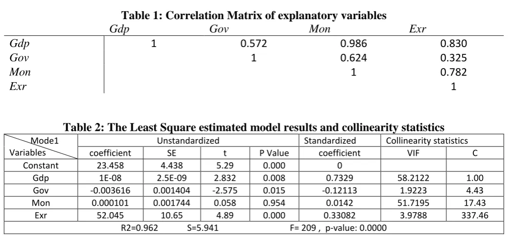
From table 2 we can see that F is highly significant (p-value-0.000), implying that the variables

chosen are valid explanatory variables, and the regression coefficient for Mon is insignificant at 5%

level of significance, also value of R2 is quite large, i.e., 0.962. Variance inflation factor (VIF,s) for all

Table 1: Correlation Matrix of explanatory variables

Gdp Gov Mon Exr

Gdp 1 0.572 0.986 0.830

Gov 1 0.624 0.325

Mon 1 0.782

Exr 1

Table 2: The Least Square estimated model results and collinearity statistics

Mode1 Variables

Unstandardized Standardized Collinearity statistics

coefficient SE t P Value coefficient VIF C

Constant 23.458 4.438 5.29 0.000 0

Gdp 1E-08 2.5E-09 2.832 0.008 0.7329 58.2122 1.00

Gov -0.003616 0.001404 -2.575 0.015 -0.12113 1.9223 4.43

Mon 0.000101 0.001744 0.058 0.954 0.0142 51.7195 17.43

Exr 52.045 10.65 4.89 0.000 0.33082 3.9788 337.46

R2=0.962 S=5.941 F= 209 , p-value: 0.0000

5.3 Application of Ridge Regression

To determine the best model fitted the data using ridge regression, firstly we present methods of choosing k.

Table 3 below summarizes the results of Ridge Regression for each method of selecting k for Inflation rate Data.

Table3: The results of Ridge Regression for each method of selecting k for Inflation rate Data

Variable

HKB LW Ridge trace

K=0.132229 K=0.09090848 K=0.489

unstandardized standardized unstandardized standardized unstandardized standardized

Intercept 23.51985 0 23.26801 0 27.13074 0

Gdp t

3.517584E-09

(8.78) 0.3640

3.696974E-09

(8.14) 0.3826

2.864229E-09

(9.56) 0.2964 Gov

t

-0.002459046

(-1.57) -0.0824

-0.002865748

(-1.86) -0.0960

-0.0004179146

(-2.72) -0.0140 Mon

t

0.002097501

(6.56) 0.2934

0.002091695

(5.87) 0.2926

0.001890136

(8.00) 0.2644 Exr

t

56.40065

(6.1) 0.3585

57.04361 (5.99)

0.3626 48.87162 _(6.48) 0.3107

R2 0.96185 0.96193 0.96122

MSE 70.43 70.44 70.40

Max VIP 1.2567 1.1611 0.4440

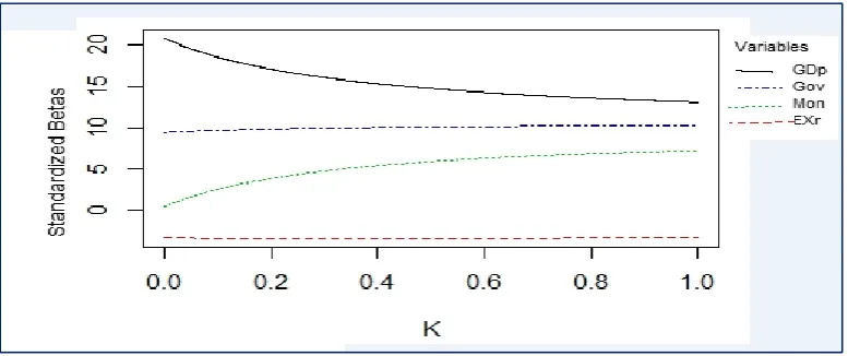
Figure 1: The values of the estimated regression coefficients plotted Against k with using ridge trace method

From table 3 above, we see that all methods for selecting k provided estimated models with significant

regression coefficients and high values of determination coefficient . Furthermore, the problem of

multicollinearity disappeared in all these models because all maximum VIF's were less than 4.

Also noting that, Lawless and Wang's method LW considers as the best method of choosing k i.e.

k=0.09091, because it has a minimum value of MSE i.e. 34.00. Therefore the estimated model of inflation by this method is:

̂

5.4 Application of The Principal Components Regression

are shown in table 4, Here the first principal components (0.555, 0.389, 0.544, 0.484)T, corresponding

to the largest eigenvalue and accounting for 77.8% of the variance is designated as PC1. The first component of this vector denotes the contribution of the first objective function towards this vector; the second component denotes the contribution of the second objective and so on.

Table 4 :The Eigenvalues and Eigenvectors

Eigenvalues ( ) 3.1107 0.7016 0.1785 0.0092

Proportion 0.778 0.175 0.045 0.002

Cumulative Proportion 0.778 0.953 0.998 1

Eigenvectors

Independent Variables

PC

PC

PC

PC

Gdp : 0.555 0.125 -0.386 -0.727

Gov : 0.389 -0.850 0.353 -0.037

Mon : 0.544 0.026 -0.478 0.681

Exr : 0.484 0.511 0.706 0.083

After obtaining, the coefficients related to the four principal components to create expressions of four PCs as

As shown in table 4, the variance of is = 0.0092 which is small and can be taken to be

approximately zero. This implies that the variable is approximately constant, and hence is equal to

its mean. Since is a linear function of standardized variables , has a mean zero. It follows that

the variable is itself approximately zero and is the source of multicollinearity. Let us exclude and

regress on , , The possible regression to be consider are

∑

Each of these models will lead to estimates all four of the original coefficients . These

estimates will be biased since has been excluded in all cases. The inclusion of would produce

exactly the same estimates as were obtained by using the LS regression of Y on all the four independent variables given in table 2.

Based on The matrix the regression equation of the dependent variable (y) on the

all-principal components Z's is

Setting = 0.530, and = = =0 in equation β=Va we get estimated β's

corresponding to the regression on the first principal component only. The estimated β's corresponding

to the first two principal components are obtain by setting = 0.530, and = = =0,

The estimates of β's corresponding to other regression are obtained in similar way. The results of all these regressions on different numbers of principal components are given in table 5

Table 5:The results of Principal components regression for Inflation rate Data

Variable

Column (1) Column (2) Column (3) Column (4)

First P.C K=1

First 2 P.C K=2

First 3 P.C K=3

All 4 P.C K=4

unstandardized standardized unstandardized standardized unstandardized standardized unstandardized standardized

Interceptt 20.07 0 18.46 0 23.29 0 23.46 0

Gdp t

2.83E-09 (14.55)

0.2926 3.27E-09 (27.24)

0.3381 3.63E-09 (11.03)

0.3761 1E-08 (2.832) 0.7329 Gov t 6.13E-03 (14.55)

0.2052 -3.11E-03 (-2.81)

-0.1042 -4.15E-03 (-2.98)

-0.1391 -0.003616 (-2.575) -0.1211 Mon t 2.09E-03 (14.55)

0.2921 2.16E-03 (26.8)

0.3015 2.49E-03 (8.5)

0.3486 0.000101 (0.058) 0.0142 Exr t 40.13 (14.55)

0.2551 69.39 (18.50)

0.4411 58.43 (5.91)

0.3714 52.05 (4.89)

0.3308

R2 0.865 0.958 0.959 0.962

Max VIP 4.400 8.431 7.271 21.282

The table shows that the difference in results obtained by using different numbers of principal components are quite substantial. As was mentioned before, the estimates in the last principal component equation( column 4 ) involving all the four possible principal components are the same as the OLS estimates.

Now we decide the number of principal components to be included in to the equation . The

rate. The first two principal components collectively explain 95.3% of the total variation in the inflation rate. Consequently, sample variation is summarized very well by two principal components. In

addition. The coefficients of and are statistically significant at 5 percent level in equation ( ).

Thus, we selected the model that based on the only first two principal components. The coefficients estimate using the principal components regression in terms of the original variables gives

t

5.5 Comparison among Least Squares, Ridge Regression, and Principal

Components Regression

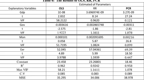
From Table 6, we see that the Multicollinearity problem between the independent variables for the inflation model has been solved by using ridge regression RR and principal components regression PCR. According to table 6, at all three methods the sign of the variable (Gov) is found to be contrary to economic theory. While the parameters of other independent variables for RR and PCR regression methods are compatible with economic theory and statistically significant, this means that the variables that have significant effect on inflation rate in Jordan during the period (1970-2007) are: Gdp, Mon, and Exr.

Table 6: The Results of OLS, RR, PCR

Estimated of Parameters

Explanatory Variables OLS RR PCR

Gdp 1E-08 3.696974E-09 3.27E-09

t 2.832 8.14 27.24

VIF 2215.55 0.9620

Gov -0.003616 -0.002865748 -0.00311

t -2.575 -1.86 -2.81

VIF 1.9223 1.1611

Mon 0.000101 0.002091695

t 0.058 5.87 26.8

VIF 51.7195 1.0824

Exr 52.045 57.04361

t 4.89 5.99 18.50

VIF 3.9788 1.5939

Constant 23.458 23.26801 18.46

R2 0.962 0.9242

Max VIF 58.21 1.078

C.V 0.085 0.083 0.089

MSE 35.295 34.006 38.978

When we compare the results of PCR method with the results of the RR in table 6, we found that PCR is better than the RR, based on the following criteria:

o The calculated values of the t-test for all parameters according to PCR are larger than those

calculated using RR method.

o The value of R2 in PCR is greater than its value in RR.

On the other hand, the RR method is considered better than the PCR method, according to the following criteria:

o The value of the coefficient of variation (C.V) of RR is less than that of PCR.

o The value of the MSE of RR is less than that of PCR method.

Generally, the results of two method RR and PCR are better than that of LS based on criteria above.

6.

Conclusions

In this paper, we have given a description of the algorithms of the two most popular biased regression methods RR and PCR. Then we discussed the connections and differences among them. RR and PCR, are proposed regression methods under collinear situation when OLS fails. They make a compromise between accuracy and precision. Their estimators are biased but with a lower mean squared estimation error. Furthermore, RR and PCR are applied to an inflation data set . The solution and performance of RR and PLR, tend to be quite similar in those practical data sets we applied. Based on the criteria of model accuracy PCR performs better than RR, whereas, according to mean squares errors criterion MSE , RR performs slightly better. In general the two biased estimator RR and PCR perform better than LS.

Reference

[1] Abdalla H. (2009).A Simulation Study Of Ridge regression Method With Auto correlated Errors.

Shendi University Journal . Issue No 6, 1-19.

[2] Ali G., Azin Z., & Pejman T. (2014). Comparing Multiple Regression ,Principal Components

Analysis ,Partial Least Square Regression and Ridge Regression in Predicting Rangeland Biomass in the Semi Steppe Rangeland of Iran. Environment and Natural Resources J .12(1), 1-21.

[3] Bro R. & Smilde K. (2003). Centering and scaling in component analysis. Journal of Chemo

metrics. 17(1), 16–3.

[4] Carl F. & Praveen K. (2002). The impact of collinearity on regression analysis: the asymmetric

effect of negative and positive correlations. Applied Econometrics. Vol 34(6), 667-677.

[5] Eledum H. (2011). Biased Estimation Methods with Autocorrelation using Simulation. LAMBERT

Academic Publishing. ISBN-137100720348-031.

[6] Frontier, S. (1976). Étude de la décroissance des valeurs propres dans une analyse en

composantes principales: comparison avec le modèle du bâton brisé. J. Exp. Mar. Biol. Ecol. 25: 67-75.

[7] Gujarati N. Damodar (2004). Basic Econometrics. Fourth Edition. McGraw-Hill. p 319.

[8] Hoerl A. E. & Kennard R.W.(1970). Ridge Regression Biased Estimation for Nonorthognal

Problems. Technometrics. 12(1), 55-67 .

[9] Hoerl A. E.,Kennard R.W., & Baldwin K.F (1975). Ridge Regression: Some Simulations.

[10] Jeffrey M. (2009).Introductory Econometrics A modern Approach. Fourth edition. South-Western-Cengage Learning. USA. P 799.

[11] Kaiser, H.F. 1960. The application of electronic computers to factor analysis. Educ. Psychol.

Meas. 20: 141-151.

[12] Kianoush F. (2013). Comparing Ridge Regression and Principal Components Regression by

Monte Carlo Simulation Based on MSE. Journal of Computer Science & Computational Mathematics. 3(2), 25-29.

[13] Lawless J.F. & Wang P. (1976). A simulation study of ridge and other regression estimators.

Communications in Statistics –Theory and Methods. 14, 1589-1604.

[14] Legendre, L. & Legendre, P. (1983). Numerical ecology. Elsevier Scientific Publishing Co. New

York. NY.

[15] Mansfield E. R., Webster J. T. & Gunst R. F.(1977). An Analytic Variable Selection Technique

for Principal Components Regression. Applied Statistics. 26(1), 34-40.

[16] Massy W.(1965). Principal Components Regression in Exploratory Research. Journal of the

American Statistical Association. 60(309), 243-265.

[17] Moawad B. (2014) .A Note on Partial Least Squares Regression for Multicollinearity (A

Comparative Study). International Journal of Applied Science and Technology Vol. 4(1), 163-170.

[18] Myres Rymond H.. )8014(.Classical and Modern Regression with Application. Ist edition. PWS

Kent Publishers. ISBN 13.0314138240041.

[19] Nawal H. (2011). Using the Method of the Mutual Integration analysis to show the effect of the

monetary and real variables in inflation through Period (1970 – 2007). Journal of Anbar University of Economic Sciences and Administration. 4(7), 179-189.

[20] Piyush K., Sarla P., & Hemlata J.(2013). Regression Analysis of Collinear Data using r-k Class

Estimator:Socio-Economic and Demographic Factors Affecting the Total Fertility Rate (TFR) in India. Journal of Data Science. Vol 11, 323-342.

[21] Xin Y. & Xiao Su.(2009).Linear Regression Analysis Theory and Computing. World Scientific.

Singapore. p 224.

[22] Yazid M. & Mowfag M. (2009). A Monte Carlo Comparison between Ridge and Principal

Components Regression Methods. Applied Mathematical Sciences. 3(42), 2085 – 2098.

[23] Zeaiter M. & Rutledge D.(2009). Preprocessing Methods. Comprehensive Chemometrics. vol.3,