3D face recognition from range images

(1)

MIAO, SHUN. 3D Face Recognition From Range Image. (Under the direction of Professor Hamid Krim).

In this thesis, we explore the statistical and geometrical behavior of the uncon-trolled parameters of a human face, including both the rigid transform caused by a head pose and the non-rigid transform caused by a facial expression. We focus on developing a 3D facial recognition scheme which is robust for these uncontrolled parameters.

This thesis presents a novel 3D face recognition method by means of the evolu-tion of iso-geodesic distance curves. Specifically, the proposed method compares two neighboring iso-geodesic distance curves, and formalizes the evolution between them as a one-dimensional function, named evolution angle function, which is Euclidean invariant. The novelty of this paper consists in formalizing a 3D face by an evolution angle functions, and in computing the distance between two faces by that of two func-tions. Experiments on Face Recognition Grand Challenge (FRGC) ver2.0 shows that our approach works very well on the neutral faces. By introducing a weight function, we also show a promising result on a non-neutral face database.

(2)

by Shun Miao

A thesis submitted to the Graduate Faculty of North Carolina State University

in partial fullfillment of the requirements for the Degree of

Master of Science

Electrical Engineering

Raleigh, North Carolina

2010

APPROVED BY:

Dr. Griff Bilbro Dr. Wesley Snyder

(3)

DEDICATION

(4)

BIOGRAPHY

Shun Miao was born in Jan. 15th 1987, to Qinan Miao and Yaling Wen, in Qing-dao, China. He received his bachelor’s degree in Electrical Engineering in 2009, from Zhejiang University, China. By a collaborate program between Zhejiang University and NC State University, he came to ECE department of NC State University for his graduate study in August, 2008. After one semester in NC State, he fortunately joined Professor Hamid Krim’s Vision, Information and Statistical Signal Theories and Applications group (VISSTA), and started working on 3D face recognition re-search.

Shun’s research focuses on pattern recognition, especially the application on face recognition. He currently emphasizes on 3D surface segmentation for detecting partial similarities.

(5)

ACKNOWLEDGMENTS

This master degree involves more than one’s brain. I wish to leave some words to reflect on the human side of my two years journey; and acknowledge all the people who contributed to the completion of this work.

My greatest thanks to my parents, who were always staying behind me, giving me as much support as they could. Father, I would never forget that you flied hundreds of miles, merely for the purpose of sitting beside a professor to inquire about educating children. And mother, it is extraordinary all those full nights you spent beside my hospital bed, giving me brave to recover from the injure. Your support helped to me go all the way to US, and to complete my Master’s work. Thank you for your love and support.

I would like to thank my advisor, Professor Hamid Krim, for all your guidance in my study and research, and your support on my PhD application. You are always very patient to listen to your students and give us valuable suggestions. I believe that what I have learned from working with you will be helpful in my whole life. Be-sides, you’ve given us extraordinary valuable opportunities to meet, on semimonthly research seminar, with world renowned scientist. Those seminar lectures helped me a lot on conducting my research. I would also like to acknowledge Professor Wesley Snyder, who took his valuable time to meet with me weekly, giving me very helpful suggestions. And thank you Professor Griff Bilbro, for you joining my advisory com-mittee. I sincerely thank to professors who have been part of my Master program, alphabetical, Prof. Winser Alexander, Prof. Brian Hughes, Prof. Xiaobiao Lin , Prof. Larry Norris and Prof. J. Keith Townsend.

(6)

LIST OF TABLES

(9)

LIST OF FIGURES

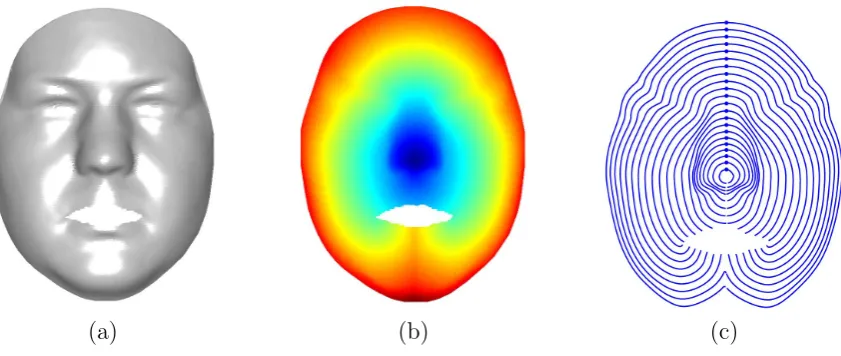
Figure 3.1 (a) Smoothed 3D face (b) Geodesic Distance Function (c) Iso-curves,

starting point is marked on each curve. To be clear . . . 12

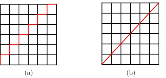
Figure 3.2 (a) Geodesic path obtained from Dijstra algorithm (b) Geodesic path obtained from Fast Marching . . . 13

Figure 3.3 Linear interpolation for detecting iso-curves . . . 14

Figure 3.4 Illustration of evolution of iso-curves. . . 15

Figure 3.5 Examples of Evolution Angle Function at different level . . . 17

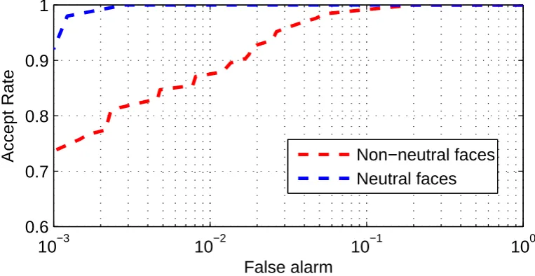
Figure 3.6 ROC curves for experiment on FRGC ver2.0 database. . . 21

Figure 4.1 Two surfaces with partial similarity . . . 29

Figure 4.2 (a) ICP registration (b) Improved ICP registration . . . 31

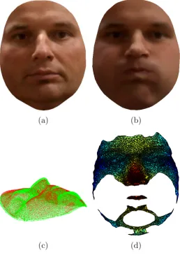
Figure 4.3 (a) Face 1 (b) Face 2 (c) Rigid surface matching between the two image (d) Segmented partial similar area . . . 32

Figure 4.4 ROC for face recognition based on improved ICP algorithm . . . 33

(10)

Chapter 1

Introduction

Face recognition is a challenging task that has been extensively researched during the last decade[1]. While most of previous face recognition works were based on 2D images, as the development of 3D scanning techniques, 3D face recognition has gained more and more attention. In a controlled environment, current 2D face recognition techniques can achieve an acceptable accuracy, but inadequate for more challenging applications, especially in the presence of variation of lighting conditions and poses [1]. 3D face recognition, by including the complete geometrical information, provides a potential to alleviate the impact of lightening and pose, and to therefore improve recognition performance.

Although more promising, the use of 3D images for face recognition also presents some challenges. First, as a surface in cartesian coordinates, a face is always subjected to Euclidean transformations, and a face alignment stage is usually required before comparison, entailing additional computational cost. Second, in most scenarios, the 3D images we have are represented by random samples on the face, or triangulation without consistent parameterizations. As a result, 3D face comparison becomes a challenging task.

(11)

of facial expressions. We proceeded to extract low dimensional features from facial range image, and built up a classifier, which can handle the deviations caused by uncontrolled parameters, such as a pose of head and a facial expression.

1.1

Motivation and Overview

In the first work of the presented thesis, we focus on modeling the evolution of facial level set curves named iso-geodesic curves, whose level set function is defined as the geodesic distance to a reference point. Our interest in the evolution of iso-geodesic curves is motivated on two counts. First, it has been shown that, change of a geodesic distance on a human face caused by facial expressions is much less than change of a Euclidean distance, and can hence be treated as an isometric transform. Therefore, the registration based on the geodesic distance is robust. Secondly, while the 3D curves are represented by cartesian coordinates that depend both on a reference and on a base, the evolution of these curves only contains intrinsic information and is Euclidean invariant. In the end, discriminant analysis is applied to evaluate the robustness of these extracted features under different facial expressions and the robust ones are selected for recognition.

(12)

square distance. We shrink the surface iteratively by removing nodes contributing large errors, until the remaining patches of the surfaces are identical. The area of matched surfaces is used as a similarity measure of these two facial images. The more area can be fitted, the more likely these images are from the same subject.

1.2

Contribution

We summarize our main contributions below.

• We have investigated the representation, classification and recognition of 3D faces under variance of facial expressions. We propose to analyze the evolution of iso-geodesic distance curves to obtain features that contain only the intrinsic geometrical information of human faces. Features of 3D faces used in the pre-sented thesis also have a nice property that they are local Euclidean invariants of a 3D surface. With the surface registration based on iso-curves, we are finally able to apply discriminant analysis techniques to select features that are robust for facial expressions.

• We introduce a 3D surface segmentation technique for searching partial

similar-ities between two facial images. With the empirical knowledge that human faces keep significant partial similarities under facial expressions, the segmentation scheme is applied to locate the invariant area between the same person’s two facial images with different facial expressions. The key idea in this problem is to iteratively expand or shrink the surface under the constrain of a mean square distance.

1.3

Outline

The present thesis is organized as follows.

(13)

pre-sented. One may distinguish these main approaches as curve cased, non-rigid surface based and template matching based approaches.

• Chapter 3 introduces a 3D face recognition algorithm based on evolution of

iso-geodesic distance curves. Both theoretical and numerical results are described in this chapter.

• Chapter 4 demonstrates a 3D surface segmentation based on the Iterative

Clos-est Point (ICP) algorithm. An improvement is made on the ICP algorithm to enable it to register partial similar surfaces.

• Chapter 5 proposes a novel framework of 3D surface segmentation as a future

(14)

Chapter 2

Background

Research interest in 3D face recognition has witnessed an explosive growth over the last few years. At first, people attempted to use 3D data to rule out variations of illumination and pose, and therefore enhance face recognition approaches based on 2D images [2][3][4][5]. There are also several works on directly applying existing 2D recognition techniques on depth images. In this chapter, we focus on the most recent and important face recognition techniques. They are categorized into three themes, a curve based, a non-rigid surface based and a template matching based approaches. Because a 3D surface is subjected to a Euclidean transformation, most 3D face recognition approaches require surface matching. A well known surface matching method is the Iterative Cloud Point (ICP) algorithm [6][7]. Feature points on faces are also widely used in surface alignment [8][9][10][11][12]. The difficulty of surface matching is clear. As human faces are not rigid surfaces, deformation will severely undermine the performance of most algorithms.

Some new ideas have recently been provided for non-rigid matching. Bronstein et al. proposed to match non-rigid surface in an isometric manner. Lu et al. [13] performed a Thin-Plate Spline warping to establish a deformable face model.

(15)

compared level set curves of geodesic distance function by developing a Euclidean invariant. Srivastavaet al. [16] measured the distance between two facial curves on a shape manifold.

Another way to avoid surface matching is to fit a template on face data. A 3D face morphable model [17] was proposed by Blanz et al., an active appearance model was proposed by Cootes et al.[18] and an annotated deformable model was proposed by Passalis et al. [19] are examples.

2.1

Curve Based Approaches

Samir et al. [14] presented a 3D face recognition method, which measures the similarity of faces on the manifold of closed planar curves. Level set curves of a depth function are extracted from 3D faces, and parameterized by arc length. A manifold of closed, arc length parameterized planar curves is generated, on which an approach of computing a geodesic on the manifold is proposed. The geodesic length between two curves on the shape manifold is used as a criterion in the nearest neighborhood recognition as the measurement of similarity. In the validation experiment, using a data set of 300 facial surfaces, 6 facial expressions each for 50 subjects, a recognition rate of 92% is reported. The method is based on depth level set curves, but depth is subjected to Euclidean transform, thus a costly alignment procedure is required.

Shuoet al.[15] proposed a Euclidean invariant for curves inR3_{to compare geodesic}

circles from 3D faces. Level set curves of a geodesic distance between any point on a face surface to nose tip are extracted, and are referred to as geodesic circles. A Euclidean integral invariant signature for curves in R3_{, which is independent for}

positions and parameterizations of curves, is presented. Based on the assumption that geodesic circles undergo piecewise Euclidean transformations on account of facial expressions, the approach is claimed to be robust to facial expressions. TheL2 _norm

(16)

rate of 95% is reported.

Mpiperis et al. [3] proposed to use geodesic polar coordinates to register faces and map the texture to the same polar system. The geodesic polar coordinates (r, θ) are defined as: radius r is the geodesic distance to nose tip, angle θ represents the tangent direction of a geodesic path at nose tip. A mapping from 3D faces to a planar surface is defined based on the geodesic polar coordinates (r, θ). The mapping

f : S1(r, θ) →S2(r, θ) is claimed to be an isometry, but which, unfortunately, is not

generally true. One experiment embeds the texture on a 3D face to a geodesic plane, and uses the flattened image for classification. Another experiment embed the depth to geodesic plane and perform classification. Experimental results are from 80.3% to 90.4% rank-one recognition rate using texture, and from 84.4% to 95% using depth, depending on the choice of database.

Srivastavaet al.[16] used the geodesic distance between geodesic circles on a shape manifold for curves in arbitrary Rn to measure the similarity between 3D faces. The pre-shape space, as a quotient space with respect to re-parametrization and rota-tion, is constructed using square-root velocity function [20][21], which can represent a curve in Rn by n functionals. An algorithm to compute a geodesic between two parameterized curves is introduced, and the geodesic distance serves as the similarity measurement for face recognition. Tested on 12 faces of 7 subjects, a recognition rate of 100% is achieved.

2.2

Non-rigid Surface Based Approaches

Bronsteinet al. [22][23] proposed an isometric model of facial expressions to allow for deformation caused by facial expressions. Based on the assumption that ”the change of the geodesic distance due to facial expressions is insignificant”, an isometric embedding is proposed to embed 3D face inR3_{, keeping the Euclidean distance in the}

(17)

a recognition rate of 100% is reported.

Li et al. proposed to use multiple features for 3D face recognition. In their first attempt [24], multiple intrinsic geometric features, including angles, geodesic distance and curvatures are extracted, and a training procedure is proposed to obtain weights for extracted features, according to their sensitivity to facial expressions. And a nearest neighbor classifier is applied using the training results as a basis. Experimental evaluation is carried out using a dataset containing 300 frontal faces, 5 faces per subject, of all the 60 subjects. The training group contains 150 faces of 30 individuals, and the test group contains the remaining 150 faces. The result showed a recognition rate of 94.17%, while rigid surface approach reaches a recognition rate of 87% on the same dataset. In their second attempt [25], a uniform remeshing scheme is proposed to extract multiple features, and a ranking procedure is applied to select expression-insensitive features. The test on the same dataset reaches a recognition rate of 94.68%.

Luet al.[13] improve previous work using a Thin-Plate Spline (TPS) approach for deformation analysis [26] to a deformable model which is able to synthesize different facial expressions from a given neutral face. 94 fiducial landmarks on 3D faces are extracted from both neutral faces and non-neutral faces in the training set, three of which are used for alignment. Given a probe face, the displacements of landmarks are added to the face, and TPS warping is applied to interpolate the deformation of landmarks to the whole surface. Tested on 877 face scans and 100 gallery tem-plates, trained by 7 independent facial expressions, a performance of 92% rank one recognition rate is achieved.

2.3

Template Matching Approaches

(18)

to face scans. The quality of the model is evaluated by the number of iterations and surface displacement. Edwards et al.[27] use this face model for face recognition. In a test with 400 faces, 200 for training and 200 for testing, a recognition rate of 88% is reported.

Similar to the idea of an active appearance model, Blanz et al. [17][28][29][30] proposed to use a 3D morphable model [31] for face recognition in both 2D and 3D. The correspondence between 3D faces and a reference face is established by the optical flow, prior to applying PCA on the reference shape and texture vectors to generate the morphable model. The illumination model of Phong is adopted to synthesize different illuminations and colors. This morphable model can reconstruct a 3D model from single 2D image. The experimental evaluation in this work uses a database with front, side and profile images in both gallery set and probe set, for a recognition rate of 99.8% for frontal-frontal case, and the lowest recognition rate of 79.5% occurs in the profile-frontal case. Huang et al. [32] added a component based approach to the morphable model, but the recognition rate remains the same.

Xu et al. [33] developed an automatic subdivision technique for consistency of a mesh. They fit a square mesh on 3D face and repeat subdivision to refine the base mesh. Gaussian-Hermite moment of shape vector is computed as feature for Nearest Neighbor classifier. Tested in a manually fitted database with 30 subjects, 6 images for each, their approach achieves a recognition rate of 96.1%. However, tested with a automatically fitted database with 60 subjects, 6 images for each, the recognition rate decreases to 72.4%.

(19)

facial expression and 40% of subjects have a variety of non-neutral facial expressions. With a false alarm rate of 10−3_{, a verification rate of 95.43% is reported on neutral}

(20)

Chapter 3

Face Recognition Using Facial

Curves

In this chapter, we develop a novel face recognition technique based on range images. We model the evolution of level set curves on a 3D surface to derive 3D Euclidean invariant features. Discriminant analysis is applied to these features to extract facial expression-insensitive features, which are used in a nearest neighbor classifier for recognition.

(21)

(a) (b) (c)

Figure 3.1: (a) Smoothed 3D face (b) Geodesic Distance Function (c) Iso-curves, starting point is marked on each curve. To be clear

3.1

Geodesic Distance Function and Iso-curves

The geodesic distance between two points on a manifold is defined as the arc length of the shortest path between these two points on the manifold. Given a 3D faceM and the nose tippnose ∈M, the Geodesic Distance Function (GDF) GM(p) is a mapping from M toRdefined asGM(p) =DM(p, pnose) whereDM(·,·) denotes the geodesic distance between two points on the manifold M. If we connect points with the same GDF value, we will obtain a set of curves, denoted as iso-geodesic distance curves (iso-curve), which are also level set curves of GDF. The iso-curve with GDF valuet can be written as (see Fig. 3.1 (a) and (b) for example)

(22)

(a) (b)

Figure 3.2: (a) Geodesic path obtained from Dijstra algorithm (b) Geodesic path obtained from Fast Marching

to error because the path is strictly constrained on the graph. One solution is to use the Fast Marching Algorithm [35] to compute the on-surface geodesic path and distance as shown in Fig. 3.2 (b). The geodesic distance computed by fast marching algorithm is the real shortest path on a triangulated surface, and is consistent to the real geodesic distance.

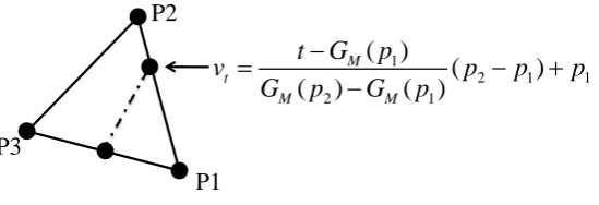
The GDF computed by fast marching algorithm is shown in Fig. 3.1 (b). Because the GDF we have is discrete, and only assumes values on vertices of a triangular mesh, we obtain an iso-curve with level C, by an approximation and interpolation. The strategy is to first obtain an edge across thet-level iso-curve, and then interpolate the edge to obtain a point. If an edge across the t-level iso-curve, it is obvious that the GDF value at one node of the edge is smaller than t, and the GDF value for the other node is greater than t. Therefore, for an edge starting from p1 and ending at

p2, the product

S(p1, p2) = (GM(p1)−t)(GM(p2)−t) (3.2)

indicates whether this edge is across the t-level iso-curve. If S(p1, p2) is negative,

(23)

P2

P3

P1

1

2 1 1

2 1

( )

( ) ( )

M t

M M

t G p

v p p p

G p G p

−

= − +

−

Figure 3.3: Linear interpolation for detecting iso-curves

iso-curves, the intersection is linearly interpolated as [36] (see Fig 3.3 for illustration).

vt =

t−GM(p1)

GM(p2)−GM(p1)

(p2−p1) +p1. (3.3)

3.2

Euclidean Invariant Evolution Angle Function

Essentially, iso-curves are level set curves defined on a manifold, with GDF as a level set function. In this section, we will discuss the evolution of these iso-curves from the perspective of differential geometry as the level valuetincreases. In Section 3.2.1, the direction of the curve evolution is analyzed and evolution vector function (EVF) is proposed to represent the curve evolution. In Section 3.2.2, by utilizing a nice property that iso-curves evolve at a constant speed, evolution angle function (EAF) is proposed to represent the 3D face in a Euclidean invariant way.

3.2.1

Evolution Vector Function

Iso-curves, as space curves, can be written as

(24)

Figure 3.4: Illustration of evolution of iso-curves.

is spanned by two orthogonal vectors. The first vector is the tangent vector of the iso-curve at the point C(s, t), denoted by T(s, t)

T(s, t) = d

dsx(s, t), d

dsy(s, t), d

dsz(s, t)

(3.5)

The other vector is orthogonal to T(s, t), denoted by B(s, t). T(s, t), B(s, t) and

N(s, t) formalize a basis of three-space, where N(s, t) denotes the normal to the surface.

The evolution speed vector E(s, t) can be decomposed into these three directions as E(s, t) = αT(s, t) +βB(s, t) +γN(s, t). Because iso-curves are constrained to the surface, the normal component γ is obviously equal to zero. The tangential component can also be set to zeros since tangential movement does not cause any change of t and it only affects the parameterization of the curve. Therefore, the evolution speed vector can simply be set to the binormal component βB(s, t), and according to the definition of an iso-curve the speed is β = 1. For simplicity, from now on, the evolution speed vector is denoted by v(s, t), and |v(s, t)|= 1.

If we extract iso-curvesci(s) = C(s, t =i∆) with a small enough ∆, the movement along directionvi(s) causes the same amount change in GDF (see Fig.3.4 for example):

(25)

approximation of evolution between the i-th iso-curve and the (i+ 1)-th one. This is an approximation because the speed vector varies in the interval ∆, and vi(s)∆ is the approximated evolution vector based on the assumption that vi(s) is a constant in the interval ∆. However, when ∆ is small enough, the approximation is quite precise and the evolution can be written as Eq.3.7. The (i+ 1)-th iso-curve has a different parameter ˆs because evolution cannot guarantee a preservation arc length parameterization.

ci(ˆs) =ci(s) +vi(s)·∆ (3.7)

3.2.2

Evolution Angle Function

Since evolution vectors are subjected to Euclidean transformations, they can hardly be used for recognition. Using the fact that the magnitude of an evolution vectors is always equal to one, we are able to represent the evolution in a Euclidean in-variant way. Because in the (T, B, N) frame, the tangential component is always zero, which means the evolution vector is in a plane that is perpendicular to the tangent vector. Because vi(s)≡ 1, the vi(s)∆ lives on a circle with radius ∆ and perpendic-ular to the tangent vector. If we are given a reference vector on this unit circle, vi(s) can be determined by an angle, which is Euclidean invariant. To generate a set of reference vectors along an iso-curve, we establish a moving frame{Ri(s), Si(s), Ti(s)} along it, whereTi(s) is the tangent vector which can be computed by the curve itself. Vectors from the nose tip to the iso-curve are denoted as qi(s), and the other two vectors are defined as:

Ri(s) =

qi(s)−qi(s) Ti(s) ||Ti(s)|| ||qi(s)−qi(s) Ti(s)

||Ti(s)||||

, Si(s) =

Ri(l)×Ti(l) ||Ri(l)×Ti(l)||

(26)

−50 0 50 −1

0 1

−50 0 50

−1 0 1

−50 0 50

−1 0 1

−50 0 50 −1

0 1

−50 0 50 −1

0 1

−100 0 100

−1 0 1

−100 0 100

−1 0 1

−100 0 100

−1 0 1

−100 0 100 −1

0 1

−100 0 100 −1

0 1

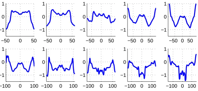
Figure 3.5: Examples of Evolution Angle Function at different level

is called an evolution angle function (EAF):

vi(s) =Ri(s) cos(θi(s)) +Si(s) sin(θi(s)) (3.8) By substituting Eq. 3.8 to Eq. 3.7, the evolution between two neighboring iso-curves is explicitly determined by EAF, which means EAFs include the necessary information needed to reconstruct the iso-curves. Given a initial Now, the problem of comparing two faces has been reduced to comparing one-dimensional functions, which is much easier because we don’t need to consider surface alignment and registration any more. A set of evolution angle functions is shown in Fig. 3.5.

3.3

Implementation

3.3.1

Face Detection and Preprocessing

(27)

of each vertex and R, G, B denote the coordinate in color space. After locating the nose tip, all vertices with distance to nose tip less than 100mm are selected to formalize a point cloud as our region of interest. Delaunay triangulation is applied to(X, Y) to generate a triangular mesh.

3.3.2

Curve Parameterization

It is obvious that Equation 3.3 only provides one point on the c-level iso-curve at a time, and we need to sort and parameterize these points to obtain a real curve. All iso-curves are arc length parameterized as α(s), s∈[a, b]. The initial point of the arc length parameterization locates on the symmetric plane of a face as shown in fig.3.1 (c), where the start points are marked as ’*’. Arc length (s) is set to be negative on the left half and position on the right half. Therefore, the absolute value |a| and |b| is the arc length of left and right half of the iso-curve, and b−a is the total arc length. Because of the diversity of arc length of iso-curves, ranges [a, b] might vary on different images and we only focus on the common range shared by all images. In simulations, iso-curves are discretized as

P[k] =P(k∆l), k= [a, b], ∆l = 2. (3.9)

3.4

Discriminant Analysis

Because of facial expressions, faces are subject to non-rigid transformation, and some part of the iso-curves are also subject to this non-rigid transformation, especially near the mouth and cheeks. Thus, only being invariant to Euclidean transform is insufficient and we need to extract features that are also robust to facial expressions. For this purpose, discriminant analysis is applied to evaluate the robustness of EAF features.

Samples of EAF is denoted as θi[k] = θi(k∆s), where i is the index of an iso-curve and ∆s the sampling interval. The within class scatter of EAF is defined as

(28)

set contains N subjects and M images for each subject, EAF of the m-th image of the n-th subject is denoted as {θ_im,n[k]}. These two scatters can be computed as

Ai[k] = 1

M

M X

m=1

(¯θ_mi [k]−θ¯i[k])2 (3.10)

Bi[k] = 1

M N

M X

m=1

(θ_m,ni [k]−θ¯i_m[k])2 (3.11) where

¯

θ_mi [k] = 1

N

N X

n=1

θ_m,ni [k], θ¯i[k] = 1

M N N X n=1 M X m=1

θ_m,ni [k] We subsequently use the same separability confidence as in [25]

Ci[k] =

Ai[k]

Bi[k]

(3.12)

It is obviously that the larger Ci[k] is, the better separability θi[k] has. After obtaining the confidence, a weighting function is defined as Eq. 3.13, which thresholds the criteria Ci_[_k_{], and only selects those features with} _C

i[k]≥γ

Wi[k] = (

0, forCi[k]< γ 1, forCi[k]≥γ

(3.13)

3.4.1

Recognition

Face recognition has two scenarios, classification and verification. In face classifi-cation, we have a face gallery withn different subjects, and given a new input image, our target is to classify this input to one of n classes in the gallery. In other words, it is a n-class classification problem. Face verification is a hypothesis test problem that given two facial images, the goal is to make decision whether they belong to the same subject. Thus, face verification is a 2-class classification problem.

(29)

˜

θi[k], is defined as Equation. 3.14:

D(θ,θ˜) =

40

X

i=1

bi X

k=ai h

(θi[k]−θ˜i[k])·wi[k]i

2

(3.14)

where, [ai, bi] is the range of the i-th iso-curve. In the next section, the Receiver Operation Characteristic (ROC) curve based on this distance measure will be shown.

3.5

Experimental Results

We collected 30 subjects as a training set from Face Recognition Grand Challenge II (FRGC2) Spring 2004 database [37]. In the training set, each subject provides 4 different expressions. Our experiment is performed on 200 images of 50 subjects. For each subject, we collected two neutral images and two non-neutral images (in-cluding smile ,surprise, inflated and frown). First, 50 neutral faces are selected as gallery templates, and 150 independent 3D scans for testing. The rank1 and rank2 recognition rate based on the matching distance is provided in Table.3.1. The match-ing distance between every pair of images (19900 in total) is computed to generate Receiver Operation Characteristic (ROC) Curve, which is shown in Fig. 3.6.

Table 3.1: Rank1 and Rank2 recognition rate Neutral faces Non-neutral faces

Rank1 100% 93.64%

(30)

10−3 10−2 10−1 100 0.6

0.7 0.8 0.9 1

False alarm

Accept Rate Non−neutral faces

Neutral faces

(31)

Chapter 4

3D Surface Segmentation

Intuitively, facial expressions only affect part of a human face, and the part re-maining invariant under expressions can be used for face recognition. In chapter 3, we extracted a set of facial curves and performed Discriminant Analysis to select expression-invariant part of these curves. In this chapter, we introduce a 3D surface segmentation scheme, which can adaptively extract identical parts between two facial images. Let’s consider two cases: the first case is that these two images are from the same subject, either of same facial expressions or different, and the second case is that the two images are from different subjects. In the first case, the extracted information is the expression-invariant part between these two facial expressions. In the second case, because it is unlikely that faces of two different subjects can share a large identical area, we have the intuition that the partial similarity between them is small. Based on this argument, the identical facial area can be used as a distance measure between two facial images.

(32)

4.1

Iterative Closest Point

A major problem of utilizing 3D data is its subjection to Euclidean transform including rotation and translation. The ICP algorithm [6][7] is a technique to register two 3D surfaces by estimating the best rigid transform between them, which minimize the mean square error (MSE). With an initial estimation of a rigid transform, the ICP algorithm iteratively chooses the corresponding point and refines the rotationR

and translation T to minimize the mean square distance.

4.1.1

Point Set Registration

A major part of ICP algorithm is the closest point registration. Given two point sets A and B, according to the closest point registration, any point in A is correspondent to the point in B with the smallest Euclidean distance to it. The mean square distance between these two point sets is defined as the average of the square Euclidean distance of all correspondent points. The Euclidean distance

d(r~1, ~r2) between two points r~1 = [x1, y1, z1]T and r~2 = [x2, y2, z2]T is d(r~1, ~r2) =

p

(x2−x1)2+ (y2−y1)2+ (z2−z1)2. For two point sets A = {a~i} and B = {b~j},

i= 1, ..., Na and j = 1, ..., Nb, the index of the correspondent point ofa∈A is

φ(i) = arg min i∈{1,...,Nb},~bi∈B

d(~a, ~bi) (4.1) Based on the closest point registration, the mean square distance between two point sets is defined as

d(A, B) = 1

Na Na X

i=1

d(a~i, ~bφ(i))2 (4.2)

(33)

4.1.2

Optimal Rigid Transformation

After registering two point sets, the ICP algorithm solves the optimal rigid trans-formation by iteratively minimizing the mean square distance as shown in Equa-tion 4.2. A well known representaEqua-tion of rotaEqua-tion in R3 _{is a 3}_×_{3 rotation matrix,}

which can be decomposed into three independent rotations in three directions,

R(θ) = 

  

1 0 0

0 cosα −sinα

0 sinα cosα

       

cosβ 0 sinβ

0 1 0

−sinβ 0 cosβ

       

cosθ −sinθ 0 sinθ cosθ 0

0 0 1



  

(4.3)

The translation is represented by a vectorT = [x, y, z]T_{. Based on the rotation matrix} and the translation vector, the Euclidean transformation of a pointxis: x0 =Rx+T. The sum of squares of distance becomes

f(R, T) = N X

i=1

||ai−Rbi−T||2 (4.4) or

f(R, T) = N X

i=1

||ai−Rbi||2−2T · N X

i=1

[ai−Rbi] +N||T||2 (4.5) The total error is obviously minimized by

T = 1

N

N X

i=1

[ai−Rbi] =µa−Rµb, (4.6) where

µa= 1

N

N X

i=1

ai, µb = 1

N

N X

i=1

bi. (4.7)

(34)

a0_i =ai−µa and b0i =bi−µb into Equation 4.4, it becomes

f(R, T) = N X

i=1

||a0_i−Rb0_i||2. (4.8) Expand the total error, we obtain

f(R, T) = N X

i=1

||a0_i||2+ 2 N X

i=1

a0_i·Rb0_i+ N X

i=1

||Rb0_i||2 (4.9) Because

||Rb0_i||2 ₌_||_b0 i||

2_, _(4.10)

minimizing the total error is equivalent to maximizing

N X

i=1

a0_i·Rb0_i. (4.11)

However, because the rotation matrix has sinusoid functions of 3 parameters, maximizing Equation 4.11 is usually very difficult. Horn et al. [38] proposed to represent the rotation by a unit quaternion ˙qR=q0+iq1+jq2+kq3, and provided a

closed form solution of Equation 4.11. His method is described as follows.

A quaternion can be thought as a complex number with three imaginary pasts, which have the following properties,

(35)

Then, the inner product of two quaternions is

˙

rq˙ = (r0qo−r1q1−r2q2−r3q3)

+i(r0q1+r1q0+r2q3−r3q2)

+j(r0q2−r1q3+r2q0+r3q1)

+k(r0q3+r1q2−r2q1+r3q0)

which can also be represented in a matrix form,

˙

rq˙ =       

r0 −r1 −r2 −r3

r1 r0 −r3 r2

r2 r3 r0 −r1

r3 −r2 r1 r0

       ˙

q =<q.˙

and

˙

qr˙ =       

r0 −r1 −r2 −r3

r1 r0 r3 −r2

r2 −r3 r0 r1

r3 r2 −r1 r0

       ˙

q = ¯<q.˙

A point (x, y, z) inR3 is represented by a quaternion ˙r=ix+jy+kz, whose real part is zero. The rotation of a point ˙r can be represented by

˙

r0 _{= ˙}_q_r_˙_q_˙_∗_{= ( ¯}_QT

Q) ˙r, (4.12)

(36)

matrix is

R(q~R) = ¯QTQ= 

  

q₀2+q₁2−q₂2−q2₃ 2(q1q2−q0q3) 2(q1q3+q0q2)

2(q1q2+q0q3) q02+q22−q21 −q32 2(q2q3−q0q1)

2(q1q3−q0q2) 2(q2q3+q0q1) q20+q32−q12−q22

    . (4.13) This representation of the rotation matrix has a polynomial form, which makes the optimization problem much easier. Now, substituting Equation 4.12 to Equation 4.11, the target function needed to be maximized becomes

N X

i=1

˙

a0_i·( ˙qb˙0_iq˙∗). (4.14) This formula cam be rewritten as

N X

i=1

( ˙qa˙0

i)·( ˙b0iq˙), (4.15) which is ˙ qT N X i=1 ¯

AT_i Bi !

˙

q, (4.16)

where Ai and Bi is the corresponding matrix of point ai and bi. Now, it is obvious that Equation 4.11 is maximized by choosing ˙q as the eigenvector corresponding to the most positive eigenvalue of the matrix

_N P i=1

¯

AT_i Bi

.

A 3×3 anti-symmetric matrix is defined as M = (P ab−

PT

ab), where P

ab = N

P i=1

a0_ib0_i, and the cyclic components of matrix M are used to form a column vector ∆ = [M23 M31 M12]T. This vector is used to compute the matrix

_N P i=1

¯

AT_i Bi . N X i=1 ¯

AT_i Bi !

=Q(P ab) =

"

tr(P

ab) ∆ T

∆ P

ab+ PT

ab−tr( P

ab)I3 #

(4.17)

(37)

eigenvec-tor q~R = [q0 q1 q2 q3]T corresponding to the maximum eigenvalue of the matrix

Q(P

ab) and the optimal translation vector is given by q~T = µ~b −R(q~R)µ~a. (For explicit proof, please see the reference [38])

4.1.3

Iterative Registration Algorithm

Given the point setA withNapoints from a data shape, and the point set B with

Nb points from a model shape, the ICP algorithm can be stated as follows. First of all, the initial registration vector p~0, named coarse alignment, is obtained by Principle

Component Analysis (PCA). For both the data shape and the model shape, three eigenvectors corresponding to three largest eigenvalues are extracted, and for each shape, there is a reference plane spanned by the first two eigenvectors. The coarse alignment is a rigid transform, which can make these two reference planes overlap, and leave the third eigenvector on the same side of the plane. After the coarse alignment, ICP algorithm is performed as follows.

1. Perform coarse alignment.

2. Obtain correspondent pairs (ai, bi) by closest point registration.

3. Estimate the registration vector by choosingq~Ras the eigenvector corresponding to the largest eigenvalue of the matrix defined in Equation 4.17, and q~T =

~

µb −R(q~R)µ~a.

4. Compute the mean square distance Dk.

5. Terminate the iteration if ||Dk−Dk−1||< λ, otherwise go back to step 2

(38)

obviously we have fk > ek+1. Therefore, the mean square distance is monotonically

decreasing as the algorithm iterates

e0 > f0 > ... > ek > fk > ek+1 > fk+1 > ... (4.18)

Thus, the ICP algorithm always converges to a local minimum.

4.2

Improvement of the ICP Algorithm

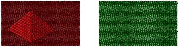
Let’s consider a very common example, which shows the limitation of the ICP algorithm. In Fig 4.1, we have two surfaces that are partially identical except for a pyramid on the red surface. Because ICP uses the mean square distance as its target function, it will definitely lead to a misalignment when there is a non-rigid deformation, as shown in Fig 4.2. However, in our face recognition applications, due to the variation of facial expressions, human faces are usually subjected to non-rigid deformation, which will severely undermine the performance of the ICP registration. In this section, an improvement of ICP is introduced to partially register non-rigid deformed surfaces.

Figure 4.1: Two surfaces with partial similarity

(39)

surface registration algorithm proposed in this section will fail. However, making ICP be able to register 3D faces under most facial expressions is also a very meaningful improvement.

Given two 3D face images of the same subject, it is the deformed areas of these two faces that undermine the ICP registration by introducing a misalignment, which cannot be canceled by a rigid transformation. Thus, the ICP algorithm will be able to provide a good surface registration if the non-rigid deformed area is removed from the surface. Intuitively, if the majority of these two triangular surface are similar, the nodes contributing the largest error belong to the deformed area. Based on this argument, we make an improvement on the the ICP algorithm by removing the most significant error contributor iteratively until the mean square distance is reduced to a pre-defined threshold λ. The improved ICP algorithm is illustrated as follows,

1. Estimate a registration vector p~= [p~R p~T]T by the ICP algorithm.

2. Compute the square error contributed by each nodebiinB,C(bi) =d(A, R(q~R)bi+

~ qT).

3. Remove bi with the largest value C(bi) from the point set B.

4. Estimate the registration vector by choosingq~Ras the eigenvector corresponding to the largest eigenvalue of the matrix defined in Equation 4.17, and q~T =

~

µb −R(q~R)µ~a.

5. Update C(bi) for each node. Compute the mean square distance as Dk = PNb

i=1C(bi).

6. Stop iteration if ||Dk−Dk−1||< µ, if not go back to step 3.

(40)

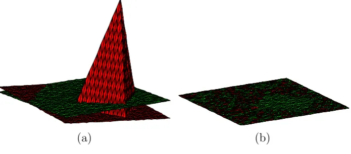
(a) (b)

Figure 4.2: (a) ICP registration (b) Improved ICP registration

4.3

Recognition and Experimental Results

The improved ICP algorithm segments identical areas between two facial images, and the area will be used for recognition. As illustrated before, it is unlikely that there are large identical areas between two different subjects, while images from the same subject usually exhibits considerably large identical areas even when they are captured under different facial expressions. Based on this observation, we simply use the size of matched area as the distance measure between facial images, and the nearest neighbor classifier is applied for classification.

(41)

(a) (b)

(c) (d)

(42)

10−3 10−2 10−1 100 0.6

0.7 0.8 0.9 1

False Alarm

Accept Rate

(43)

Chapter 5

Future Work in 3D Segmentation

by the Level Set Method

As stated before, the improved ICP algorithm is based on an assumption that the majority of a face area will remain invariant under most facial expressions. When certain extreme facial expressions violate this assumption, the improved ICP algo-rithm might fail. In this chapter, we propose to use level set method for detecting partial similarity between facial images. Given two 3D facial images, the general idea is to grow a level set curve on one given facial image, with the constrain that the facial areas inside the level set curve is identical to a subset of the other image. The initialization of the level set curve is a rectangular around the nose tip, which is expression-insensitive even under extreme facial expressions. Then the level curve evolves on the face to absorb more area, which is identical to the other image. The evolution is guided by an Eikonal partial differential equation, and solved by a fast marching method.

(44)

discussed in Section 5.3.

5.1

Background

5.1.1

Level Set Method

Level set method was first proposed by Osher and Sethian [39][35]. In this sub-section, some of the basic concepts and implementation details of level set method are introduced. A level set curve defined by a level set function φ(x, y, t) is a path (x(t), y(t)) on which the level set value must be zero. Hence,

φ(x(t), y(t), t) = 0. (5.1) By the chain rule,

φt+∇φ(x, y)·~v(x, y) = 0, (5.2) where~v(x, y) = [x0(t), y0(t)]. IfF supplies the speed in the outward normal direction, then F =~v ·~n, where~n =∇φ/|∇φ|. The evolution equation forφ is

φt+F|∇φ|= 0. (5.3)

Given an interface identified as a level set curve of the level set function φ, Equa-tion 5.3 describes the time evoluEqua-tion of the interface. Consider a special and simple case where the level set function φ(x, y) is defined as the time at which the interface crosses the point (x, y), denoted as T(x, y). In this special case, the derivative of the level set function with respect to time t is always equal to 1, thus Equation 5.3 becomes a partial differential equation,

|∇T|F = 1. (5.4)

(45)

the initialization curve.

Because usually we need to solve the eikonal equation on a image plane, where the domain is divided into grid points sampled in bothxandydirection, it’s necessary to construct an accurate approximation of the gradients ∇T. An upwind scheme given in [40] is shown to be a very efficient and precise approximation of the gradients. The level set functionT(x, y) can be expanded as a Taylor series in bothxandydirection, thus we have

T(x+ ∆, y) = T(x, y) + ∂T(x, y)

∂x ∆ +O(∆

2₎

T(x, y+ ∆) =T(x, y) + ∂T(x, y)

∂y ∆ +O(∆

2₎

After rearranging this expression, the derivative at point (x, y) can be written as

Tx(x, y) =

T(x+ ∆, y)−T(x, y)

∆ +O(∆)

Then, differential operators are defined as

D+xT = T(x+ ∆, y)−T(x, y)

∆ ,

D−xT = T(x, y)−T(x−∆, y)

∆ , (5.5)

D0xT = T(x+ ∆, y)−T(x−∆, y)

2∆ .

According to the upwind scheme, only values upwind of the direction of information propagation should be used. Therefore, the gradient is approximated by

|∇T| = [max(D−_i xj,0)2+ min(D+_i xj,0)2,

(46)

Substitute Equation 5.6 into Equation 5.4, we can obtain,

1

F2 = max(D

−x i j,0)

2 _{+ min(}_D+x i j,0)

2_,

+ max(D_i−yj,0)2+ min(D_i+yj,0)2. (5.7) A similar approximation to the gradient was introduced by Rouy and Tourin [41],

1

F2 = max max(D

−x i j,0)

2

,−min(D+_i xj,0)2,

+ max max(D−_i yj,0)2,−min(D+_i yj,0)2. (5.8)

5.1.2

Fast Marching Method

A very efficient numerical solution of the Eikonal equation, named fast marching algorithm was proposed by Sethian [35]. For this discussion, we limit ourselves to a positive speed function F(x, y), which makes the level set curve monotonically propagate off the initial line.

The key of fast marching algorithm is that the upwind different structure means the information propagates “one way”, from smaller values of T(x, y) to larger ones, which meets the assumption of a positive speed function. Because the idea of fast marching method is to update the value T(x, y) around the existing front iteratively, the selection of which grid to update around the front is the key of the whole algo-rithm. Because of the assumption that the front propagates “one way”, the smallest value around the front is always correct; other points around the front with larger

T(x, y) cannot affect it. The technique is explained algorithmically as follows, 1. Definition

(a) Alive points: points whose value of T(x, y) is known for sure. Letting (i, j) denote the index of grid, the set of alive points is represented by Ω ={(i, j)}.

(47)

(i+ 1, j), (i, j−1), (i, j+ 1)). The value ofT at the Narrow Band points are estimated by Equation 5.8.

(c) Far away points: points which are neither alive points nor narrow band points. The value of T at the Far Away points are set to be infinity. 2. Fast Marching Algorithm

(a) Begin Loop: Let (imin, jmin) be the point inNarrow Band with the smallest value for T.

(b) Add the point (imin, jmin) to the Ω, and remove it from Narrow Band. (c) Tag as neighbors any points (imin−1, jmin), (imin+1, jmin), (imin, jmin−1),

(imin, jmin + 1) that are either in Narrow Band or Far Away. All these neighbors are them moved to the Narrow Band set.

(d) Recompute the values ofT at all neighbors according to the largest possible solution to the quadratic equation (Equation 5.8).

(e) Return to the top of the loop

Because the recomputed T is selected to be that largest possible solution to the quadratic equation, whenever converting a Narrow Band point to Alive, the process of recomputing theT value of its neighbors cannot produce a value less than anyAlive value. This property guarantee that the level set curve is always marching ahead in time.

The discrete form of Equation 5.8 is given by

f_ij2 = max max(D−_i xj,0)2,−min(D_i+xj,0)2,

+ max max(D_i−yj,0)2,−min(D+_i yj,0)2, (5.9) where the inverse of speed function Fij is replaced by fij = _F12. Consider a the

matrix of grid values in Fig. 5.1 from [35]. The goal is to compute the new value of

(48)

B

A

?

C

D

Figure 5.1: Matrix of adjacent grids

generality, the value A is assumed to be the smallest value of T in the Narrow Band set. The problem can be generally divided into to cases.

case 1: C is not alive. In this case, the T value of the center grid should be computed fromA.

1. If A+f ≤min(B, D), Tcomputed= (A+f).

2. If A+f > min(B, D), with out loosing generality, we assume that B <= D. The value ofT is obtained by solving the quadratic equation (Tcomputed−A)2+ (Tcomputed−B)2 =f2

case 2: C is alive. In this case, theT value of the center grid should be computed fromC. This case defaults into the first case above.

5.2

Surface Segmentation by Solving Eikonal

Equa-tion

As discussed above, the algorithm introduced in Section 4.2 cannot cope with extreme facial expressions, as the invariance of the majority of facial area is not valid. Our future work will be focused on the surface segmentation scheme based on the level set method, which is much more robust under extreme facial expressions.

(49)

not uniform sampled. Thus, as a preprocessing procedure, (X, Y, Z) is uniformly sampled to generate depth image z[i, j] =f(i∆, j∆), wherei, j denotes the discrete

x, y coordinates.

By the depth images, the 3D segmentation can be performed by segmenting the parameter space of (x, y), which can be formalized by a level set method. The seg-mentation of the a 3D face is represented by a level set function T(x, y). Given a level value c, the surface is segmented into two parts: Sin(c) = {(x, y)|T(x, y) ≤ c} andSout(c) ={(x, y)|T(x, y)> c}, whereSin is the region inside the c-level set curve, and Sout is the region outside it. In this section, we select appropriate speed vector in order to make Sin to be the facial region which is invariant to the presented facial expression, and Sout to be the region which undergoes a non-rigid deformation.

To solve the Eikonal equation, a boundary condition is needed. As shown by Chang, K.I. et al. [42], the nose region is the most stable part of human face which remains invariant under extreme facial expressions. In other words, given two 3D facial images A and B of the same subject, a small area around the nose tip in A

(50)

as follows,

1. Detect a rectangular region near nose tip, Sin(0),as the boundary condition of the Eikonal equation. According to fast marching algorithm, Sin is the Alive set. Based on this, initialize the Narrow Band and the Far Away sets.

2. Beginning of the loop: Estimate registration vector ~p= [p~R p~T]T betweenSin and B by the ICP algorithm. Perform the rotation R(p~R) and the translation

~

pT on the surface A.

3. Compute the distance from each node {x, y, z =f(x, y)} inA toB, denoted as

D(x, y).

4. Set F(x, y) to be F(x, y) = _D₍_x,y1 ₎λ. And f(x, y) =D(x, y) λ_.

5. Let (imin, jmin) be the point inNarrow Band with the smallest value forT. Add the point (imin, jmin) to theSin, and remove it from Narrow Band.

6. Tag as neighbors any points (imin −1, jmin), (imin + 1, jmin), (imin, jmin −1), (imin, jmin+1) that are either inNarrow Band orFar Away. All these neighbors are them moved to the Narrow Band set.

7. Recompute the values of T at all neighbors according to the largest possible solution to the quadratic equation (Equation 5.8).

8. Return to the top of the loop

5.3

Discussion and Future Work

The form of the speed function F(x, y) has very a significant impact on the evo-lution result. Thus, one part of the future work is the selection of the speed function

(51)

used as a measurement of the surface similarity, and the speed functionF(x, y) is set to be a monotonically decreasing function of D(x, y). However, some more complex similarity measurements, like curvature or shape index, might be better. Thus, it is necessary to analyze the performance of these similarity measurements, as well as other forms of the speed function F(x, y).

(52)

Bibliography

[1] Andrea F. Abate, Michele Nappi, Daniel Riccio, and Gabriele Sabatino. 2d and 3d face recognition: A survey. Pattern Recognition Letters, 28(14):1885 – 1906, 2007.

[2] Xiaoguang Lu, Rein-Lien Hsu, A.K. Jain, B. Parsi, and B. Kamgar-Parsi. Face recognition with 3d model-based synthesis. In Biometric Authenti-cation. First International Conference, ICBA 2004. Proceedings (Lecture Notes in Comput. Sci. Vol.3072), pages 139–46, 2004.

[3] I. Mpiperis, S. Malassiotis, and M.G. Strintzis. 3-d face recognition with the geodesic polar representation. Information Forensics and Security, IEEE Trans-actions on, 2(3):537–547, Sept. 2007.

[4] F. Tsalakanidou, D. Tzovaras, and M. G. Strintzis. Use of depth and colour eigenfaces for face recognition.Pattern Recognition Letters, 24(9-10):1427 – 1435, 2003.

[5] Bernard Achermann, Xiaoyi Jiang, and Horst Bunke. Face recognition using range images. Virtual Systems and MultiMedia, International Conference on, 0:129, 1997.

(53)

[7] Zhengyou Zhang. Iterative point matching for registration of free-form curves and surfaces. International Journal of Computer Vision, 13(2):119 – 52, 1994.

[8] D. Colbry, G. Stockman, and Anil Jain. Detection of anchor points for 3d face veri.cation. In Computer Vision and Pattern Recognition - Workshops. IEEE Computer Society Conference on, pages 118–118, June 2005.

[9] C. Dorai and A.K. Jain. Cosmos-a representation scheme for 3d free-form objects. Pattern Analysis and Machine Intelligence, IEEE Transactions on, 19(10):1115– 1130, Oct 1997.

[10] G. Gordon. Face recognition based on depth maps and surface curvature. Geo-metric Methods in Computer Vision, SPIE, 1991.

[11] A.B. Moreno, A. S?chez, E. Fr?s-Mart?ez, and J.F. V?ez. Three-dimensional facial surface modeling applied to recognition. Engineering Applications of Ar-tificial Intelligence, 22(8):1233 – 1244, 2009.

[12] Alessandro Colombo, Claudio Cusano, and Raimondo Schettini. 3d face detec-tion using curvature analysis. Pattern Recognition, 39(3):444–455, 2006.

[13] Xiaoguang Lu and A.K. Jain. Deformation modeling for robust 3d face matching. Pattern Analysis and Machine Intelligence, IEEE Transactions on, 30(8):1346– 1357, Aug. 2008.

[14] C. Samir, A. Srivastava, and M. Daoudi. Three-dimensional face recognition using shapes of facial curves. Pattern Analysis and Machine Intelligence, IEEE Transactions on, 28(11):1858–1863, Nov. 2006.

(54)

[16] A. Srivastava, C. Samir, S. H. Joshi, and M. Daoudi. Elastic shape models for face analysis using curvilinear coordinates.Journal of Mathematical Imaging and Vision, pages 253–265, June 2008.

[17] V. Blanz and T. Vetter. Face recognition based on fitting a 3d morphable model. Pattern Analysis and Machine Intelligence, IEEE Transactions on, 25(9):1063– 1074, Sept. 2003.

[18] T.F. Cootes, G.J. Edwards, and C.J. Taylor. Active appearance models. Pattern Analysis and Machine Intelligence, IEEE Transactions on, 23(6):681–685, Jun 2001.

[19] G. Passalis, I.A. Kakadiaris, T. Theoharis, G. Toderici, and N. Murtuza. Eval-uation of 3d face recognition in the presence of facial expressions: an annotated deformable model approach. InComputer Vision and Pattern Recognition, IEEE Computer Society Conference on, pages 171–171, June 2005.

[20] S.H. Joshi, E. Klassen, A. Srivastava, and I. Jermyn. Removing shape-preserving transformations in square-root elastic (sre) framework for shape analysis of curves. InEnergy Minimization Methods in Computer Vision and Pattern Recog-nition. Proceedings 6th International Conference, pages 388–98, 2007.

[21] S.H. Joshi, E. Klassen, A. Srivastava, and I. Jermyn. A novel representation for riemannian analysis of elastic curves in rn. In Computer Vision and Pattern Recognition, IEEE Conference on, pages 1–7, June 2007.

[22] A.M. Bronstein, M.M. Bronstein, and R. Kimmel. Expression-invariant repre-sentations of faces. Image Processing, IEEE Transactions on, 16(1):188–197, Jan. 2007.

(55)

[24] Xiaoxing Li and Hao Zhang. Adapting geometric attributes for expression-invariant 3d face recognition. In Shape Modeling and Applications, IEEE In-ternational Conference on, pages 21–32, June 2007.

[25] Xiaoxing Li, Tao Jia, and Hao Zhang. Expression-insensitive 3d face recogni-tion using sparse representarecogni-tion. In Computer Vision and Pattern Recognition Workshops, 2009. CVPR Workshops 2009. IEEE Computer Society Conference on, pages 2575–2582, June 2009.

[26] Xiaoguang Lu and A.K. Jain. Deformation analysis for 3d face matching. In Application of Computer Vision, IEEE Workshops on, volume 1, pages 99–104, Jan. 2005.

[27] G.J. Edwards, T.F. Cootes, and C.J. Taylor. Face recognition using active ap-pearance models. In Computer Vision - ECCV’98. 5th European Conference on Computer Vision. Proceedings, volume vol.2, pages 581–95, 1998.

[28] J. Huang, V. Blanz, and B. Heisele. Face recognition using component-based svm classification and morphable models. InProceedings of Pattern Recognition with Support Vector Machines. First International Workshop., pages 334–41, 2002.

[29] S. Romdhani, V. Blanz, and T. Vetter. Face identification by fitting a 3d mor-phable model using linear shape and texture error functions. In 7th European Conference on Computer Vision. Proceedings, Part IV, pages 3–19, 2002.

[30] V. Blanz, S. Romdhani, and T. Vetter. Face identification across different poses and illuminations with a 3d morphable model. In Automatic Face and Gesture Recognition, IEEE International Conference on, volume 0, page 0202, 2002.

(56)

[32] J. Huang, B. Heisele, and V. Blanz. Component-based face recognition with 3d morphable models. In Audio- and Video-Based Biometric Person Authentica-tion. 4th International Conference, AVBPA 2003. Proceedings (Lecture Notes in Computer Science Vol.2688), pages 27–34, 2003.

[33] Chenghua Xu, Yunhong Wang, Tieniu Tan, and Long Quan. Automatic 3d face recognition combining global geometric features with local shape variation infor-mation. In Proceedings of Sixth IEEE International Conference on Automatic Face and Gesture Recognition, pages 308–13, 2004.

[34] I.A. Kakadiaris, G. Passalis, G. Toderici, M.N. Murtuza, Yunliang Lu, N. Karam-patziakis, and T. Theoharis. Three-dimensional face recognition in the presence of facial expressions: An annotated deformable model approach. Pattern Analy-sis and Machine Intelligence, IEEE Transactions on, 29(4):640–649, April 2007.

[35] J. A. Sethian. A fast marching level set method for monotonically advancing fronts. Proceedings of the National Academy of Sciences of the United States of America, 93(4):1591–1595, 1996.

[36] S. Feng, H. Krim, and I. A. Kogan. 3d face recognition using euclidean integral invariants signature. In Statistical Signal Processing, 2007. SSP ’07. IEEE/SP 14th Workshop on, pages 156–160, Aug. 2007.

[37] P.J. Phillips, P.J. Flynn, T. Scruggs, K.W. Bowyer, Jin Chang, K. Hoffman, J. Marques, Jaesik Min, and W. Worek. Overview of the face recognition grand challenge. In Computer Vision and Pattern Recognition, 2005. CVPR 2005. IEEE Computer Society Conference on, volume 1, pages 947–954 vol. 1, June 2005.

(57)

[39] Stanley Osher and James A Sethian. Fronts propagating with curvature-dependent speed: Algorithms based on hamilton-jacobi formulations. Journal of Computational Physics, 79(1):12 – 49, 1988.

[40] J. A. Sethian. Level set methods and fast marching methods - evolving inter-faces in computational geometry, fluid mechanics, computer vision, and materials science. In Interfaces in Computational Geometry, Fluid Mechanics, Computer Vision, and Materials Science. Cambridge University Press, 1998.

[41] Elisabeth Rouy and Agns Tourin. A viscosity solutions approach to shape-from-shading. SIAM Journal on Numerical Analysis, 29(3):867–884, 1992.