Volume 2008, Article ID 370524,15pages doi:10.1155/2008/370524
Research Article
A Method to Estimate the Horizontal Handover Decision Effect
on Indoor Wireless Conversational Video Quality
Alfonso Fernandez Duran,1Raquel Perez Leal,2and Jose I. Alonso2
1Alcatel-Lucent Spain, Ramirez de Prado 5, 28045 Madrid, Spain
2Escuela Tecnica Superior de Ingenieros de Telecomunicacion, Universidad Politecnica de Madrid, Ciudad Universitaria,
28040 Madrid, Spain
Correspondence should be addressed to Alfonso Fernandez Duran,alfonso.fernandez [email protected]
Received 1 October 2007; Revised 31 January 2008; Accepted 4 April 2008
Recommended by Jianfei Cai
One of the most interesting and valuable services considered in fixed mobile convergence is video telephony. The success of this conversational video service will depend on the conversational video quality achieved in the multicell wireless indoor scenarios. One of the essential elements in the quality is the effect of the horizontal handovers in the conversational video. This paper analyzes the handover decision based on the probability calculation of handover events in the case of relative signal strength with hysteresis threshold (RSSHT) approach, and it proposes a new handover decision mechanism, variable hysteresis, to avoid unnecessary handovers. The paper presents the impact of the number of handovers and their duration time on the video’s effective frame rate. Moreover, the effect of video stream modification during a short handover is also analyzed. Probability and handover duration approaches are combined and a new simple method for video quality evaluation is caused by the handovers in multicell indoor WLAN scenarios. Finally, the model proposed has been applied to a real office scenario.
Copyright © 2008 Alfonso Fernandez Duran et al. This is an open access article distributed under the Creative Commons Attribution License, which permits unrestricted use, distribution, and reproduction in any medium, provided the original work is properly cited.
1. INTRODUCTION
In the current context of fixed-mobile convergence, WLAN technology based on 802.11 is becoming available in common portable and mobile user terminals. This has brought about the possibility of using WLAN technology in conversational applications. Although IEEE802.11 was
originally intended to transport best-effort data traffic,
the incorporation of new standards like IEEE802.11e has brought about the opportunity of deploying delay and bandwidth sensitive services, like real-time voice and video communications. In these circumstances, WLANs combined with IP are being used as technology for limited mobility and nomadic services. The success of this scenario will depend on maintaining the communication’s continuity through networks with several wireless access points (APs) by means of horizontal handover. WLANs were not initially designed to support handover between access points, based on the fact that users will most probably remain within the networks in a rather stationary way, using nonreal-time services. The normal use of a WLAN typically supports nonreal-time
handovers between APs, provided that the users have access rights to the destination network. The handover consists of an association to a wireless AP once the network client enters the coverage area of the destination AP. The horizontal handover is therefore a break before make process. User terminals usually incorporate just one WLAN transceiver,
but in the case where two transceivers could be used, [1]
describes a mechanism to manage handovers based on the voice over IP packet transmission retries. Horizontal
handover is addressed in IEEE802.11r, [2]. The first dealing
with authorization issues between different networks, and
the second with increasing speed in the handover between access points.
The horizontal handover process could be split into two steps. The first one is to decide whether a handover is necessary and then select the destination AP. The second covers the layer 2 and layer 3 processes. The first step could take place in parallel with the communication without
affecting it, while the second takes time from the service
being conveyed. A description of the message transactions
to [1] layer 2 could take between 50 milliseconds and 400 milliseconds, while layer 3, depending on the network settings could take 300 milliseconds or more.
Several studies have analyzed the handover decision pro-cess in cellular communications. Studies of the propagation parameters and criteria followed in handover decisions in
cellular networks could be found in [4–7]. These studies are
mainly related to outdoor mobile communications. Other studies characterize the performance of the handover in
WLANs as based on measurements like [8], that characterize
the timings and data transfers between network elements,
and [9] measure the effects of handovers in voice
communi-cations. The impact of the horizontal and vertical handovers
in voice communications is studied in [10] using the E model
from ITU G.107.
Regarding video services, as a consequence of the evolution of the technologies and applications, advanced coding techniques have been introduced as a video coding
format. In this study, ITU-T Rec. H.264|ISO/IEC
14496-10 and H.264 have been considered. H.264 “represents an evolution of the existing video coding standards (H.261, H.262, and H.263) and it was developed in response to the growing need for higher compression of moving pictures for various applications such as videoconferencing, digital storage media, television broadcasting, Internet streaming,
and communication” [11].
The H.264 defines a limited subset of syntax called “pro-files” and “levels” in order to facilitate video data interchange
between different applications. A “profile” specifies a set of
coding tools or algorithms that can be used in generating a conforming bitstream, whereas a “level” imposes constraints on certain key parameters of the bitstream. The recommen-dation defines seven profiles (Baseline, Extended, Main and four High-profile types) and fifteen “levels” per “profile.” The same set of “levels” is defined for all “profiles.”
Current studies show that handovers have an impact on the quality of communications, since handovers pro-duce discontinuities in the communication data streams. A discussion on video, the packet sizes and the implications
in the PSNR are presented in [12]. The results shown
are based only on simulations, and no model is proposed to predict the system performance. A qualitative study of using an intelligent access point handover mechanism in WLAN to obtain user perception for video conferencing quality, before and after applying the intelligent access point
handover mechanism is presented in [13]. This reference
shows that some strategies could improve the handover performance when the APs are congested, however no
models are proposed to predict the effect on the video
communications performances. In the case of conversational video, it is possible to obtain a simple video quality estimator
using the effective frame rate resulting from the packet losses
due to the handover effect, as introduced in reference [14].
Therefore, it is very appropriate to analyze the impact of handover on video communications quality in order to better understand the process involved. Moreover, it is also necessary to improve the method of planning real handover scenarios while maintaining the communication quality. The conversational video degradation due to the handover
processes taking place in a wireless network can be addressed from at least two general perspectives: video processing to
minimize whatever effect is taking place in the transmission
media, and wireless processing carried out in the wireless part. With regard to the radio part, a new decision handover mechanism has been proposed (called variable hysteresis) to reduce unnecessary handovers. Moreover, in the video part, video stream modification has been introduced to minimize the handover duration impact arising from the interdependency of video frames. The following sections introduce the framework for conversational video applica-tion handover, a new and simple method of conversaapplica-tional video quality estimation based on handover time duration is also proposed. Finally, quality evaluation is shown in a real
office scenario and planning recommendation provided.
2. WLAN HANDOVER PRINCIPLES
WLANs belonging to the IEEE802.11 family were not originally conceived to support a fast handover between access points. This has become a drawback when deploying multi-AP networks that convey real-time conversational services like IP-based video and voice telephony. The issue comes from the fact that the time necessary to associate it to a new AP is neither controlled nor limited to short-time intervals. The association short-time could be of several
hundreds of milliseconds as shown in [8,15], while quality
of communications such as voice could be severely affected
by handover times of more than 50 milliseconds [10]. In
addition, the availability of resources at the destination AP is not known until the handover has taken place. To solve these issues, the IEEE802.11r workgroup was set up to define a protocol to enable a fast and reliable handover between access points. By means of this new protocol, the mobile node (MN) can establish security and QoS status before taking a transition decision.
IEEE 802.11u is another IEEE task group that was set up to allow devices to interconnect with external networks, as typically found in hotspots. The main goal of this task group is to produce an amendment to the IEEE 802.11 standard to allow a common approach to interconnecting IEEE 802.11 access networks to external networks in a generic and standardized manner. The main particular issues covered are network selection, emergency call support, authorization from subscriber network, and media independent handover support.
2.1. Signal strength
variable following a lognormal distribution as described in,
[4,5,16,17] in the following form:
fi(s)= 1
sσi
√
2πe
−(s−μ
i)
2 /2σ2
i, (1)
wheresis the received signal amplitude of the envelope,μi
are the average signal losses received at the mobile node from
the wireless access pointi, and could be expressed as
μi=k1+k2log
di
, (2)
where di represents the distances from the observation
point to the wireless access pointi, APi. Constants k1 and
k2 represent frequency dependent and fixed attenuation
factors, and the propagation constant, respectively. Finally,σi
represents the shadowing that could be reasonably averaged to express slow power variations.
Although (1) represents the fading probability
distri-bution function for the path losses as described in (2), in
complex scenarios, such as indoors, in which many obstacles make up the propagation losses, the signal strength could be expressed as
μi=Ptx−
k1+
k
λk+k2log
di
, (3)
whereλk is the attenuation of the kpassing through walls
in the path from the observation point to the wireless access
point, andPtxthe transmitted power. Moreover, to take the
attenuation into account due to different floors in indoor
propagation, one additional term could be added to (3) as
stated in [18].
Other possible choices of statistical distributions for modeling the envelope have been described and detailed studies, based on exhaustive measurements, have been carried out to characterize indoor propagation. The Weibull distribution appears to be one of the statistical models that best describes the fading amplitude and fading power indoor
scenarios, [18–21] , improving the lognormal distribution in
many cases. The Weibull distribution could be expressed as
fi(s)=ba−bsb−1e−(s/a)bI(0,∞)(s), (4)
wheresrepresents the fading amplitude envelope or the
fad-ing power, andaandbare the position and shape values of
the distribution, respectively. When the power distribution is represented in dBm, the extreme value distribution function
should be used. In fact, ifs has a Weibull distribution with
parametersaandb, log(s) has an extreme value distribution
with parametersμ=log(a) andσ=1/bas shown in [22,23].
The extreme value function for the power probability distribution function (pdf) has been seen as a good
approxi-mation. An example of fitting is shown inFigure 1. As can be
seen, the power histogram of an indoor trajectory, modeled
by the lognormal pdf function, is sufficiently represented by
the extreme value function.
This behavior has already been observed in scenarios with complex propagation conditions such as vegetation
obstacles [24].
0 0.05 0.1 0.15 0.2 0.25
Densit
y
−95 −90 −85 −80 −75 −70 −65 −60 Signal strength (dBm)
Extreme value fit Lognormal fit
Figure1: Comparison of lognormal and extreme value pdf fit for an indoor trajectory power log.
0 0.1 0.2 0.3 0.4 0.5 0.6 0.7 0.8 0.9 1
C
u
m
ulati
ve
pr
obabilit
y
−95 −90 −85 −80 −75 −70 −65 −60 Signal strength (dBm)
Sample cdf from trajectory Extreme value approximation Lognormal approximation
Figure2: Comparison of lognormal and extreme-value cumulative distribution approximation for an indoor trajectory power log.
Since most of the analysis will be probabilistic, it is
interesting to see how the histogram inFigure 1is
approx-imated in terms of cumulative distribution function (cdf).
The comparison results are shown in Figure 2.
Integrat-ing the differences between the sample data and the cdf
approximations, an overall error of 2% can be seen for the case of lognormal function, and 5.5% for the case of extreme value function. Although lognormal is better overall in this scenario, local analysis shows that the maximum
difference between sample data and lognormal cdf is 0.24,
while the maximum difference for the extreme value is 0.16.
us to derive analytical expressions for the handover factors involved.
The extreme value probability distribution function is commonly used in the modeling and analysis of phenomena with low occurrence probabilities, as in risk analysis or the study of meteorology.
The pdf of the extreme value distribution can be expressed as
fi(s)= 1
σie
(s−μi)/σie−e(s−μi)/σi, (5)
whereσiandμiare as defined above.
To analyze the strategies for the handover decision in outdoor cellular communications in the case of microcells
and macrocells, [4,6,16] base their analysis on the
estima-tion of the probability of unnecessary handovers from the statistical power distributions. For example, in the case of two base stations, what would be the probability of handover from base station 1 to 2 and then from 2 back to 1. In the case of indoor WLAN deployments, the conditions of simultaneous coverage of several access points, in which unnecessary handovers could take place between several of them, for instance from AP1 to AP2, from AP2 to AP3, and the back to AP1 are very frequent. The estimation of
handover efficiency based on unnecessary handovers then
becomes very complicated, as unnecessary handovers are
very difficult to distinguish from necessary ones using the
transition logic.
An alternative way of analyzing the handovers in outdoor communications is by means of the residence time, that is, once a handover has taken place, how long the mobile node
stays in the new base station. In [25], the residence time
statistics for handovers are analyzed. In the case of an indoor
WLAN, the size of the cells also makes it very difficult to
distinguish handovers based on the residence time, since a normal walking speed could produce a relatively high number of valid handovers with a relatively low residence time.
2.2. Handover decision techniques
As an alternative to the analysis carried out for cellular communications, the present study proposes a simple anal-ysis of the handover probability founded on the metrics used to make the handover decision in indoor WLAN communications. It is assumed that the scenario has been
properly planned to provide sufficient coverage (minimum
signal strength guaranteed at least in one of the access points). The strategy providing a lower probability of handover will present an overall better performance from the communication quality point of view. Based on these principles, several techniques could be used to implement the handover decision. In the following sections, these techniques are presented in order to introduce progressively the mathematical expressions to be used later in the method proposed.
2.2.1. Best server handover
If a mobile node sees the power levels si from each access
points APiwithin the coverage range, if no other criteria are
implemented, it will associate itself to the one with higher average power. Assuming that the mobile node is currently
at AP0, it will hand over to another APiif there is one such as
si> s0. In this case, the mobile node will carry out handovers on best server basis.
The probability of a handover taking place will be
PHO=
n
i=1
Pi
si> s0
. (6)
Since the cumulative distribution function of (5) has a
closed form
F(s)=1−e−e(s−μ)/σ
. (7)
Therefore,
Probs > s0
=1−Probs < s0
. (8)
Consequently,
Probs > s0
=1−1−e−e(s0−μ)/σ
=e−e(s0−μ)/σ . (9)
Combining (6) and (9), the probability of having a
handover will be given by
PHO=
n
i=1
e−e(s0−μi)/σi
, (10)
where the mobile node is associated to AP0 and
simultane-ously receives a signal strength above the sensitivity threshold
fromnaccess points{AP1, AP2,. . .APn}.
The main advantage of the best server approach is that it always keeps the mobile node associated to the AP giving the best signal quality, and therefore the higher bandwidth. On the other hand, the main disadvantage is that the number of handovers taking place during a mobile node moving trajectory could be very high, and therefore communications quality issues could take place, especially, in real-time conversational services.
Practical handover decision approaches usually require a reduction in the number of handovers taking place, while keeping the signal strength as high as possible.
2.2.2. Handover with fixed Hysteresis
A common approach to reduce the total number of han-dovers is to use a fixed hysteresis. The mechanism consists of carrying out a handover to a new AP, when the signal
strength has improved over certainh value. If the current
AP has a signal strengths0, the handover to the new APiwill
happen ifsi> s0+h.
Figure 3 shows the basic behavior of the hysteresis handover. While the best server approach will produce
a handover decision at point A, hysteresis approach will
−70
−65
−60
−55
−50
−45
−40
Si
gn
al
st
re
ngth
(dBm)
0 5 10 15 20 25
Distance (m) Current AP
Destination AP Hysteresis
h A
B
Figure3: Signal strength and handover with hysteresis.
point B. This approach absorbs any potential unnecessary
handover originated with improvements lower thanhon the
signal quality.
Following the same approach as in the case of the best server, the probability of having a handover will be
PHO=
n
i=1
Pi
si> s0+h
. (11)
This could be expressed in a closed form as
PHO=
n
i=1
e−e(s0 +h−μi)/σi
. (12)
In the particular case that same statistics are assumed for
then+ 1 access points in a network, and replacings0with the
expected value (μ),hcould be expressed in a closed form as
h=σln
ln
n P
. (13)
As can be seen, hdepends on the number of access points
(n), the probability of having a handover and the standard
deviation of the signal strength distribution, but it does not
depend on the average signal strength (μ). From (13), it
appears that h depends mainly on the standard deviation
of the signal strength, with influence from the number of access points. Notice that the reduction in the probability
of having a handover requires an increase ofh. Similarly, h
has to increase in networks with a larger number of access points.
The plain hysteresis approach described has the implicit drawback of producing a certain amount of unnecessary handovers, when the signal strength from the current access
point is high, and the ratiosi> s0+his still possible.
2.2.3. RSSHT handover
An improvement over the plain hysteresis handover decision approach is used to reduce the unnecessary handovers, when the signal strength of the current access point is high enough. The improved technique is known as relative signal strength with hysteresis and threshold (RSSHT). This technique is
described in [8], and it basically allows a handover of the type
si> s0+hwhens0> TCS, beingTCSthe signal threshold. The probability of handover in this case could be expressed as
PHO= ⎧ ⎪ ⎪ ⎨ ⎪ ⎪ ⎩
n
i=1
Pi
si> s0+h
∀s0≤TCS,
0 ∀s0> TCS,
(14)
or in a closed form:
PHO= ⎧ ⎪ ⎪ ⎨ ⎪ ⎪ ⎩
n
i=1
e−e(s0−μi)/σi ∀
s0≤TCS,
0 ∀s0> TCS.
(15)
The selection of the hysteresis marginhcould be carried
out in the same way as in the plain hysteresis approach. Using RSSHT, it is possible to reduce the total number of handovers. The probability of having a handover for a given signal strength in the current AP will be influenced by the
proper selection of theTCS value. A possibility of selecting
a TCS value could be to estimate the signal strength for a
given probability of crossing TCS for a given access point.
For example, assuming the same power distribution in all the access points, an estimation of the threshold could be
TCS=μ+σln
−ln1−PCS
, (16)
wherePCS (probability of crossing the threshold) could be
taken as the same value used for the probability of handover
in the estimation ofhin (13).
Since a reduction in the number of handovers is pos-sible using RSSHT, this technique is commonly used in commercial products. Nevertheless, there is still a remaining
part of handovers that are produced nearTCS and are also
unnecessary.
2.2.4. Handover with variable hysteresis
To increase the performance of conversational video in multicell wireless networks in the presence of handovers, we propose an improvement based on the use of hysteresis techniques with a variable margin. In such a way that when signal strength is high, the probability of a handover
taking place is reduced (increase in thehvalue), and when
signal strength is lower, the probability of handover increases
(decrease in the h value). This approach will minimize
the effect of having unnecessary handovers nearTCS using
RSSHT.
To obtain a variable hysteresis margin, let us define a
lower signal strength reference, calledsT, this value could be
−80
−70
−60
−50
−40
−30
−20
−10
Si
gn
al
st
re
ngth
(dBm)
0 10 20 30 40 50
Distance (m) Current AP
Target AP
Fixed hysteresis Variable hysteresis
h h C
D Variable
hysteresis
Variable hysteresis
Figure4: Variable Hysteresis behavior.
s0−sT, wheres0is the current AP0signal strength. Assuming
that APiis the handover destination mobile node candidate
andsiis the power level received from it; handover only will
take place ifsi>2s0−sT, that is, the higher the signal strength,
the higher the hysteresis margin, and therefore the lower the probability of a handover taking place will be.
The behavior of the variable hysteresis is compared to the
plain hysteresis inFigure 4, where it is noticeable that the
handovers that took place at pointC andD are no longer
necessary, since the variable hysteresis line does not cross the
power level of the target AP. This effect is possible since the
minimum signal strength of the current AP is rather high. In these conditions, the probability of a handover taking place will be
PHO=
n
i=1
Pi
si> s0+s0−sT
=
n
i=1
Pi
si>2s0−sT
. (17)
This could be expressed in a closed form as
PHO=
n
i=1
e−e(2s0−sT−μi)/σi
. (18)
Just as in the case of plain hysteresis, assuming that all signal distributions are similar, the lower reference signal strength could be estimated as
sT=μ−σln
ln
n P
. (19)
The lower bound value is also a function of the expected
value μ, therefore the selection of this value could depend
on how the actual network has been deployed, and could be
taken as sT = μ−h, using h as in the plain hysteresis or
RSSHT cases.
All of the handover techniques described could produce an abnormal behavior in conditions, where none of the access points available are received with a minimum amount of signal strength. These are typical conditions when outage conditions are produced.
2.3. Signal outage conditions
A critical situation will occur when a mobile node such as a handheld device exits, the WLAN, for instance moving outside the coverage area. In this case, the way to keep the communication continuity is whenever possible to carry out a vertical handover to a cellular network.
If sS is the signal level threshold to have acceptable
communication in the WLAN, the probability that APi is
received at the mobile node with a signal below this level will be
Psi< sS
=FsS
=1−e−e(sS−μi)/σi
. (20)
The condition for outage will be met, when all access points are below the threshold value. This condition could be expressed as
PVH=
n
i=0
Psi< sS
, (21)
or in a closed form:
PVH=
n
i=0
1−e−e(sS−μi)/σi
. (22)
In these conditions, the mobile node should have decided a vertical handover with certain anticipation. Descriptions of several techniques used for anticipating the vertical handover
decision are available in [26]. Proper WLAN deployment
designs should maintain the probability of experiencing outages and therefore vertical handovers in the coverage area in low values.
2.4. Comparison of handover decision approaches
The different handover approaches described could be
compared by making some simplifying assumptions, and evaluating the probability of experiencing a handover for a given current access point signal strength value. Provided that the minimum acceptable signal strength is achievable, the lower the probability of having a handover is, the better the performance is, and therefore the better the associated approach.
Assuming that all access points present the same signal strength statistical behavior, and being consistent with the
results of Figures 1 and 2 with μ = −70 dBm, σ = 10,
and usingh = 10 dB andsT = −92 dBm for a scenario of
four access points, the results for the different approaches are
shown inFigure 5.
As can be seen, the probability of a handover taking place for a given signal strength is higher for the case of the best server approach, while minimum for the case of variable
hysteresis. The difference between RSSHT and hysteresis
appears within the lower handover probability range, caused by the threshold, and in the others both curves are identical and appear to overlap. In these conditions, it performs better than RSSHT, the latter better than hysteresis and hysteresis
performs better than the best server. The differences are
maintained in the whole range of the power values.
Taking the same values, the probability of signal outage
0 0.1 0.2 0.3 0.4 0.5 0.6 0.7 0.8 0.9 1
HO
pr
obabilit
y
−92 −82 −72 −62 −52
Signal level at current AP (dBm) Best server
Hysteresis 10 dB
RSSHT
Variable hysteresis Model comparison for a four access point deployment
Figure5: Comparison of the different handover approaches.
3. CONVERSATIONAL VIDEO PERFORMANCE
A usual approach to estimating video quality is the peak signal-to-noise ratio (PSNR), or more recently video quality rating (VRQ) both are usually estimated from the mean square error (MSE) of the video frames after the impairments (e.g., packet loss) with respect to the original video frames
[27,28]. From these values, there is some correlation to the
video mean opinion score (MOS), unfortunately, the rela-tionship between packet loss and MSE is not straightforward, since not all packets conveyed through the wireless network have the same significance. Alternatively, a relatively simpler
quality indicator is proposed in [14]. This indicator is the
effective frame rate, which is introduced and discussed in
later sections of this paper. This paper also proposes a model
to characterize the impact of packet losses on the effective
frame rate of the video sequence.
As packet losses occur in the wireless network, video frames are damaged; making some of them unusable, and therefore the total frame rate is reduced. Video quality will be acceptable, if the expected frame rate of the video conversations is kept above certain value.
The consequence of a packet loss in a generic video sequence depends on the particular location of the erroneous packet in the compressed video sequence. The reason for this is related to how compressed video is transmitted through the IP protocol. The plain video source frames are compressed to form a new sequence of compressed video frames or slices. The new sequence could be, depending on the H.264 service profile applied, made up of three types of frames: I (Intra) that transports the content of a complete
frame with lower compression ratio, P (Predictive) that
transports basic information on an prediction of the next
frame based on movement estimators, andB(Bidirectional)
that transports the difference between the preceding and the
following frame. This sequence of slices is grouped into the so-called group of pictures (GoPs) or groups of video (GoV) objects depending on the standard. The GoV could adopt many forms and structures, but for our analysis, we assume a typical configuration of the form IPBBPBBPBBPBBPBB. This means that every 16 frames there is an Intra followed
by Predictive and Bidirectional frames. IP video packets are built from pieces of the aforementioned frame types and delivered to the network. If a packet error has been produced
in a packet belonging to an Intra frame, the result is different
from the same error produced in a packet belonging to a Predictive or Bidirectional frame.
There are some characteristics that are applicable to the case of conversational video, and in particular to portable conversational video, that are not necessarily applicable to other video services like IPTV or video streaming. The first important characteristic is the low-speed and low-resolution formats (common intermediate format, CIF, or quarter CIF, QCIF), that in turn produce a very low number of
packets per frame, especially, if protocol efficiency is taken
into account by increasing the average packet size. In these conditions, a single packet could convey a substantial part of a video frame. The second important characteristic comes from the portability and low consumption requirement at the receiving end that in turn requires a lighter processing load to save battery life. The combination of the two aforementioned characteristics makes packet losses impact greatly on the frame integrity and concealment becomes very restrictive. In conversational video, it could be better for instance to maintain a clear fixed image of the other speaker on the screen, than to try error compensation at the risk of severe image distortions and artifacts. Following these characteristics, every time that a packet is lost in a frame, the complete frame becomes unusable, and some actions could
be taken at the decoder end to mitigate the effect, such as
freezing or copying frames, but the effective frame rate has
been reduced and has to accept some form of video quality degradation.
It is possible to obtain a simple video quality estimator
based on the effective frame rate resulting from the packet
losses due to the handover effect, as introduced in [14].
Although this could not be generalized for all types of IP video, in the case of conversational video, this indicator presents advantages over the use of PSNR: allows simple relationship between the packet loss and objective quality, and intuitively represents the behavior of conversational video over a wireless network.
3.1. Handover impact on video quality
In the present analysis, it is considered that the handover
durationTsis longer than a video frame. Typical handover
durations can be found in [15]. When the handover duration
affects several slices, the video stream can only be displayed
once an I frame is received, as shown inFigure 6. IfTsis the
GoV andThis the handover duration, two cases are possible
when Th< Ts and the handover event involves slices from
two GoV or whenTh> Ts. For the rest of the analysis, it is
considered thatTh< Ts, (e.g.,Th < 1000 milliseconds) and
therefore the number of frames lost are always less than two GoVs.
B B P B B P B B I
IP B B P B B P B B P B B P B B I B B P B B P B BIIP B B P B B P B B P B B P B BIIP B B P B B P B B P B B P B BIIP B B P B B P B B P B B P B BI
B B P B B P B B I
IP B B P B B P B B P B B P B B I B B P B B P B B I
B B P B B P B B I
IP B B P B B P B B P B B P B B I IP B B P B B P B B P B B P B B I B B P B B P B BIIP B B P B B P B B P B B P B BIIP B B P B B P B B P B B P B BIIP B B P B B P B B P B B P B BI B B P B B P B BIIP B B P B B P B B P B B P B BIIP B B P B B P B B P B B P B BI
B B P B B P B BI
B B P B B P B BIIIP B B P B B P B B P B B P B BP B B P B B P B B P B B P B BIIIIP B B P B B P B B P B B P B BP B B P B B P B B P B B P B BIIIIP B B P B B P B B P B B P B BP B B P B B P B B P B B P B BII
Th< Tsand I slice involved orTh> Ts
Handover event Th: HO duration (s)
I-frame
I-frame I-frame
Ts(s) Ts(s)
As displayed
Must wait until I-frame here is received Video stream as transmitted GoV:nsslices GoV:nsslices
Figure6: Handover effect on displayed video stream.
expected number of frames lost will depend in the position of the handover initiation in the GoV, which can be expressed as
E1= 1
ns ns−1
i=0
ns−i
. (23)
Depending on the handover duration, it is possible that the handover takes place at the end of one GoV, taking the first
slices of the next, which makes GoV unusable. This effect
produces an additional expected number of lost frames, which could be expressed as
E2= 1
ns nh
j=1
ns, (24)
wherenh is the handover duration expressed in number of
slices, that could be calculated from
nh=ceil
Thf0
, (25)
whereThis the handover duration, and f0is the video frame
rate.
The expected number of frames lost in the video sequence due to a handover will be
E=E1+E2=ns
2 +nh−1. (26)
The performance of video in terms of frame rate in the presence of handovers could be expressed as follows:
f =f0
1−E·PHO
. (27)
The performance will depend on the handover technique used. If the RSSHT technique is used, the resulting frame rate
obtained bycombining (15), (26), and (27) will be
f = f0
1−
ns
2 +nh−1
n
i=1
e−e(s0−μi)/σi
∀s0≤TCS. (28)
If variable hysteresis is used, by combining (18), (26), and
(27) the resulting frame rate will come from
f = f0
1−
ns
2 +nh−1
n
i=1
e−e(2s0−sT−μi)/σi
. (29)
The previous approach is also applicable to the case of signal outage conditions, that is, none of the access points
is received above the sensitivity threshold. In this case, (27)
becomes
f =f0
1−E·PHO+PVH
. (30)
Since signal outage is produced when no handover is
possible, in the case of signal outage, (30) becomes
f = f0
1−
ns
2 +nh−1
n
i=0
1−e−e(sS−μi)/σi . (31)
Equation (31) is valid for the cases in which the signal
outage duration is longer than one video frame, which is the
typical case. This effect is mainly related to the radio network
design and could have very low impact.
In Figures 7 and 8, the case of four cells is shown.
According to the signal levels, there is certain probability of experiencing a handover, and thus undergoing a reduction in the frame rate. The example covers several handover durations. If the acceptability limit is considered to be
5 frames/second [29], quality outage can be evaluated as
a function of the signal strength coming from the radio network design.
It must be noted that in Figure 7 outage starts at
−76 dBm, while inFigure 8it appears at−79 dBm, which is
a 3 dB improvement.
3.2. Solution to improve handover impact on video quality
0 2 4 6 8 10 12 14 16 18
Exp
ect
ed
fr
ame
rat
e
−81 −79 −77 −75 −73 −71
Signal level at current AP (dBm) 70 ms
200 ms
600 ms 1000 ms
Acceptability limit
Figure7: Frame rate as a function of the signal quality according to handover probability in multicell networks in the case of RSSHT.
0 2 4 6 8 10 12 14 16 18
Exp
ect
ed
fr
ame
rat
e
−81 −79 −77 −75 −73 −71
Signal level at current AP (dBm) 70 ms
200 ms
600 ms 1000 ms
Acceptability limit
Figure8: Frame rate as a function of the signal quality according to handover probability in multicell networks in the case of variable hysteresis.
from at least two general perspectives: video processing to
mitigate whatever effect is taking place in the transmission
media, For example, degradations due to channel, han-dovers, call drops, and so forth, and wireless processing carried out in the wireless part. In the previous section, the variable hysteresis handover technique has been proposed in order to minimize the handover probability, in this section the solution proposed focuses on the video part.
In fact, a technique that could improve the video quality caused by handover will be to reduce the GoV objects lost due to frame interdependence. This will be possible by forcing
a reset of the GoV to generate an I frame, breaking off
the natural sequence of frames IPBBPBBPBBPBBPBB and reducing the time between I frames. An example is shown inFigure 9.
There are, at least, two possible techniques to implement the proposed reset. First, to take advantage of channel reci-procity for conversational video, which means that down-and uplinks channel behaviors are closely related, so the
transmitter end can detect a handover event automatically as well as generating the I frame automatically when required. Another technique will be to introduce a feedback from receiver to transmitter through a real-time control protocol.
In these conditions, the new expected value of frames lost in the process will consist of at least one frame lost to detect the event and an additional frame to reset the GoV. On top of these 2 frames, the total duration of the handover will need to be translated in a frame count.
Taking as example the RSSHT case, (28) will become
f = f0
1−nh+ 2
n
i=1
e−e(s0−μi)/σi
∀s0≤TCS. (32)
As a result, there will be a considerable statistical improvement in the case of short handovers, while this improvement is smaller in the typical case of longer handovers; in any case, it also depends on the relative distance between the handover end event and the next
Intra-frame. Figure 10 compares the different approaches
discussed in terms of expected frame rate as a function of the average signal level received at the AP. The expected
frame rate represents the effective frame rate resulting from
the packet losses due to the handover effect. Handover
duration is 1000 milliseconds in Figure 10. The shape of
the curves is strongly influenced by the handover technique used. Variable hysteresis produces softer shape, while RSSHT produces a somehow abrupt behavior. As can be seen, the greater improvement is achieved with the variable hysteresis approach although some additional improvement is also possible combining both variable hysteresis and Intra reset. Most of the gain is produced by the use of variable hysteresis, as will be confirmed by simulations.
4. SCENARIO SIMULATION
To illustrate the principles shown in the above sections,
an example has been selected as shown in Figure 11. The
scenario corresponds to an office environment of 20.2×35.5
meters covered with four access points represented with the color shapes inside the layout, each color associated to a frequency channel. The walls have been modeled to introduce attenuation in the signal propagation and edge
diffraction. The position of the access points has been
found with an automatic process to optimize the coverage and capacity simultaneously. The dashed line represents a trajectory of a mobile node at 4 Km/h in the scenario, covering a total distance of 190 m.
The handover performance could be assessed for the
different conditions described in the previous sections. The
simulations consist of the use of RSSHT and of variable
hysteresis techniques with different handover durations
through the trajectory and comparing the results. The power histograms of the four access points through the trajectory
are shown in Figure 12. Several iterations are also carried
B B P B B P B B II P B B P B B P B B P B B P B B II P B B P B B P B B P B B P B B I
B B P B B P B B I
I P B B P B B P B B P B B P B B I B B P B B P B B IIP B B P B B P B B P B I P B B P B B P B B P B B P B BI I B B P B B P B B II P B B P B B P B B P B B P B B II P B B P B B P B B P B B P B B I
B B P B B P B B I
I P B B P B B P B B P B B P B B I B B P B B P B B IIP B B P B B P B B P B I P B B P B B P B B P B B P B BI I B B P B B P B B II P B B P B B P B B P B B P B B II P B B P B B P B B P B B P B B I
B B P B B P B B I
I P B B P B B P B B P B B P B B I B B P B B P B B IIP B B P B B P B B P B I
B B P B B P B B II P B B P B B P B B P B B P B B II P B B P B B P B B P B B P B B I
B B P B B P B B I
I P B B P B B P B B P B B P B B I B B P B B P B B IIP B B P B B P B B P B I
B B P B B P B B II P B B P B B P B B P B B P B B II P B B P B B P B B P B B P B B I B B P B B P B B I
B B P B B P B B III P B B P B B P B B P B B P B BP B B P B B P B B P B B P B B IIII P B B P B B P B B P B B P B BP B B P B B P B B P B B P B B II
B B P B B P B B I B B P B B P B B I
I P B B P B B P B B P B B P B B I I P B B P B B P B B P B B P B B I B B P B B P B B I
B B P B B P B B IIP B B P B B P B B P B IIII P B B P B B P B B P B B P B BP B B P B B P B B P B B P B BP B B P B B P B B P B B P B BP B B P B B P B B P B B P B BI IIII
Handover event
Th: HO duration (s)
I-frame
“Forced”
I-frame “Natural” I-frame
L(s) L(s)
As displayed Natural video
stream GoV:nsslices GoV:nsslices
Intrareset video stream as transmitted
Figure9: Handover effect on displayed video stream with Intra reset.
0 2 4 6 8 10 12 14 16 18
Exp
ect
ed
fr
ame
rat
e
−81 −79 −77 −75 −73 −71
Signal level at current AP (dBm) Variable hysteresis
RSSHT
Variable hysteresis intra reset RSSHT intra reset
Acceptability limit
Figure10: Frame rate performance for 1 second handovers using the different techniques.
1 2
3
4 20.2 m
35.5 m
Figure11: Simulation scenario.
4.1. RSSHT handover parameter simulation
The use of a threshold above, where no handover action takes place, produces some improvement in the total number of handover events, even without using hysteresis, this is due to the simple fact that some of the best server handovers
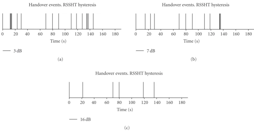
are taking place at relatively high signal strengths.Figure 13
represents handover events as a function of time to move through the trajectory by the mobile node at a pedestrian
speed. As shown inFigure 13, the total number of handovers
for the 3 dB margin is reduced from 25 to 17, and with 7 dB the reduction is from 17 to 12. An additional margin increases to 16 dB, produces a further reduction in the total handover events down to 6, but at the expense of having the lowest signal strength below the system sensitivity. Just as in the case of plain hysteresis, in this case the distribution of
handover events also depends onh, and the increase inhis
stripping handovers from the registry, and slightly changing their position.
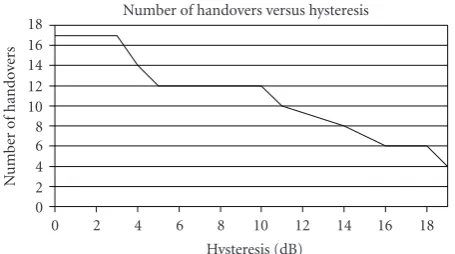
The impact of the hysteresis margin on the number of
handover events using threshold is shown inFigure 14. The
behavior is monotonic down to 19 dB where 4 handovers are produced; an additional increase in the margin produces no improvement in the handover count.
Although the number of handovers decrease monoton-ically as the hysteresis margin increases, it is essential to
analyze the impact on the minimum signal level. The effect
of the hysteresis margin on the minimum signal strength
value is shown in Figure 15. The use of a threshold has
less influence on the minimum signal strength observed. Hysteresis greater than 9 dB produces minimum signal strength in the range of the system sensitivity, therefore a
0 0.02 0.04 0.06 0.008.1 0.12 0.14 0.16 0.018.2
− 90 − 88 − 85 − 83 − 80 − 78 − 75 − 73 − 70 − 68 − 65 − 63 − 60 − 58 − 55 − 53 − 50 − 48 − 45 − 43 AP1 (a) 0 0.02 0.04 0.06 0.08 0.1 0.12 0.14 0.16
− 91 − 88 − 86 − 84 − 81 − 79 − 77 − 75 − 72 − 70 − 68 − 65 − 63 − 61 − 58 − 56 − 54 − 52 − 49 − 47 AP2 (b) 0 0.02 0.04 0.06 0.08 0.1 0.12 0.14 0.16
− 91 − 89 − 87 − 85 − 83 − 81 − 79 − 77 − 75 − 73 − 71 − 69 − 67 − 65 − 63 − 61 − 59 − 57 − 55 − 53 AP3 (c) 0 0.02 0.04 0.06 0.08 0.1 0.12 0.14 0.16
− 91 − 89 − 86 − 84 − 82 − 80 − 77 − 75 − 73 − 71 − 69 − 66 − 64 − 62 − 60 − 57 − 55 − 53 − 51 − 48 AP4 (d)
Figure12: Power histograms for the four APs through the trajectory.
0 20 40 60 80 100 120 140 160 180 Time (s)
3 dB
Handover events. RSSHT hysteresis
(a)
0 20 40 60 80 100 120 140 160 180 Time (s)
7 dB
Handover events. RSSHT hysteresis
(b)
0 20 40 60 80 100 120 140 160 180 Time (s)
16 dB
Handover events. RSSHT hysteresis
(c)
Figure13: Handover events using RSSHT.
us take 7 dB, since it is producing a minimum signal in the
range of−86 dBm.
Summarizing, thehvalue has to be as small as possible to
keep the minimum signal level as high as possible, but at the
same timehhas to be as large as possible to reduce the total
handover count. The tradeoffselected has beenh=7 dB.
4.2. Variable hysteresis simulation
One of the advantages of the variable hysteresis techniques is that there is no need for parameter tuning. The only
parameter is the lower boundary that can be the system
sensitivity threshold that is usually −92 dBm for typical
IEEE802.11 WLAN.
Figure 16 shows the results obtained using variable hysteresis in the reference scenario. As can be seen, the number of handovers has been reduced from 12 (optimal RSSHT with hysteresis of 7 dB) to 9 keeping the same value of minimum signal strength in the trajectory.
0 2 4 6 8 10 12 14 16 18
N
u
mb
er
of
hando
vers
0 2 4 6 8 10 12 14 16 18
Hysteresis (dB) Number of handovers versus hysteresis
Figure14: Handover events as a function of the hysteresis margin usingTCS= −80 dBm.
−95
−93
−91
−89
−87
−85
−83
−81
−79
−77
−75
M
inim
um
po
w
er
le
vel
(dBm)
0 2 4 6 8 10 12 14 16 18
Hysteresis (dB) Minimum signal level versus hysteresis
Figure15: Minimum signal strength as a function of the hysteresis margin forTCS= −75 dBm.
5. SCENARIO PERFORMANCE RESULTS
Taking the RSSHT handover technique with the parameter setting from the previous sections, it is possible to analyze the impact of the handovers in the conversational video quality.
The approach followed has been to simulate the video
performance for different handover durations in the scenario
shown inFigure 11.
Assuming that the total duration of the trajectory is 171 seconds, corresponding to a relative low moving speed, the average frame rate of the conversational video obtained in
different handover durations is shown inFigure 17.
The fluctuations of the frame rate are due to the frames lost in the handover process. Depending of the duration of the handovers and the frequency of the occurrence, the frame rate can be reduced down to values that are not acceptable for the user. If the generally accepted value of 5 frames/second
[29] is taken as figure of merit for video acceptability, it is
possible to see how the frame rate evolves and where it will
cross the limit.Figure 17presents this circumstances starting
at 134 seconds for all handover durations. This effect is due
to the accumulation of handovers starting at this point of the
trajectory, as can be seen inFigure 13, not allowing the video
frame rate to recover.
If the frame rate drops to 5 frames/second or below, it is considered as producing an outage, and the outage ends once
0 20 40 60 80 100 120 140 160 180 Time (s)
−92 dBm
Handover events. Variable hysteresis threshold
Figure16: Handover using variable hysteresis.
0 2 4 6 8 10 12 14 16 18
F
rame
rat
e
(fps)
0 20 40 60 80 100 120 140 160
Trajectory time (s) 70 ms
200 ms 500 ms
100 ms 300 ms 1000 ms
Figure 17: Resulting frame rate as a function of the handover duration using RSSHT.
the frame rate raises again above 5 frames/second. Using this principle, the duration of the quality outages can be estimated.
By repeating the process for different handover
dura-tions, it is possible to assess the influence of the handover duration on the quality outages.
If GoV reset is applied, the results are significantly
improved as shown inFigure 18.
Figure 19shows the effect of the handover duration on the outage in the simulation scenario for normal RSSHT and RSSHT with Intra reset. As can be seen, the quality outage grows monotonically with the handover duration as expected.
In the present simulation, it is noticeable that handover durations longer than 600 milliseconds produce a relatively flat quality outage in RSSHT, this means that above 600 milliseconds the outage of 7.5% of time is obtained no matter how long the handover is (up to the simulated value of 1000 milliseconds). To explain this behavior, it is necessary to
revisitFigure 13. It is clearly visible that an accumulation of
handovers can be seen at the end of the trajectory. These handover events are due to a sequence of abrupt signal fluctuations received from two of the access points (AP3
and AP4) in the scenario. This effect is partially mitigated
by using the GoV reset in the low range of the handover duration, as it can be expected.
0 2 4 6 8 10 12 14 16 18
F
rame
rat
e
(fps)
0 20 40 60 80 100 120 140 160
Trajectory time (s) 70 ms
200 ms 500 ms
100 ms 300 ms 1000 ms
Figure 18: Resulting frame rate as a function of the handover duration using RSSHT with GoV reset.
0 1 2 3 4 5 6 7 8
Outage
time
(%)
50 250 450 650 850
Handover duration (ms) w/o intra reset
Intra reset
RSSHT handover
Figure 19: Quality outage time as a function of the handover duration.
frames per second in all cases which is way above the acceptability limit. The average frame rate experiences rather low reductions thanks to the positions of the handover events that are rather spread along the trajectory
A final comparison has been performed simulating PSNR as indicator to validate the results obtained. To use PSNR as quality indicator, it is necessary to use a known video sequence and for that purposes the “Foreman” sequence has been used. For the simulations, the following parameters have been considered: QCIF test sequence “Foreman” (25 frames/second, 300 frames), mobile user at 4 Km/h, com-pressed bit rate at 32 Kbps and average handover duration of 1000 milliseconds. Since “Foreman” is shorter than the duration of the simulated trajectory, the video sequence has been concatenated several times. The technique used for received frame lost concealment is the frame copying, that is, an interval of lost frames is replaced by the last usable frame received.
The results obtained repeating the process for the
different techniques, and averaging between handover events
are shown in Figure 21. Average PSNR at 32 Kbps bit
rate without handover is 31 dB [30] and a 25 dB PSNR
acceptability limit is assumed.Figure 21shows similar results
as for the case of frame rate. In fact, the outage appears at
0 2 4 6 8 10 12 14 16 18
F
rame
rat
e
(fps)
0 20 40 60 80 100 120 140 160
Trajectory time (s) 70 ms
200 ms 500 ms
100 ms 300 ms 1000 ms
Figure 20: Resulting frame rate as a function of the handover duration using variable hysteresis.
0 5 10 15 20 25 30 35
PSNR
(dB)
0 20 40 60 80 100 120 140 160
Trajectory time (s) RSSHT
PSNR
Variable hysteresis RSSHT-intra reset
Acceptability limit
Figure21: Simulated PSNR using Foreman video sequence.
the end of the path with both RSSHT techniques, with and without Intra reset, however variable hysteresis solves this problem.
6. CONCLUSIONS AND FUTURE WORK
The effect of horizontal handover on the conversational
grow with the handover duration. The improvement coming from the video stream modification has been compared with those coming from variable hysteresis handover decision technique: the new technique proposed at this paper. The results show that improvements in the handover process reducing unnecessary handovers produces higher quality gain than the video transport processing.
Subsequent research steps will be, first, a more profound performance analysis and simulation of the variable hys-tereris handover decision mechanisms to further reduce the handover count in multicell deployments to increase the quality. Second, to introduce new video quality indicators that could also be applicable to video streaming and mobile TV.
ACKNOWLEDGMENTS
The authors are thankful for the support of the Spanish Min-istry of Education and Science within the framework of the TEC2005-07010-C02-01/TCM and the TSI2005-07306-C02-01/CASERTEL-NGN projects chair in Madrid Polytechnic University. The authors are also thankful for the support of CELTIC Project Easy Wireless II.
REFERENCES
[1] S. Kashihara and Y. Oie, “Handover management based on the number of retries for VoIP on WLANs,” inProceedings of the 61st IEEE Vehicular Technology Conference (VTC ’05), vol. 4, pp. 2201–2206, Stockholm, Sweden, May-June 2005.
[2] Draft Standard for Information Technology Telecommuni-cations and informationexchange between systems—Local and metropolitan area networks—Specific requirements— part 11: Wireless LAN Medium AccessControl (MAC) and Physical Layer (PHY) specifications—Amendment 2: Fast BSS Transition. Active Unapproved Draft.
[3] A. Mishra, M. Shin, and W. Arbaugh, “An empirical analysis of the IEEE 802.11 MAC layer handoffprocess,” Computer Communication Review, vol. 33, no. 2, pp. 93–102, 2003. [4] M. Zonoozi and P. Dassanayake, “Handover delay and
hys-teresis margin in microcells and macrocells,” inProceedings of the 8th IEEE International Symposium on Personal, Indoor and Mobile Radio Communications (PIMRC ’97), vol. 2, pp. 396– 400, Helsinki, Finland, September 1997.
[5] M. Gudmundson, “Analysis of handover algorithms [micro-cellular radio],” in Proceedings of the 41st IEEE Vehicular Technology Conference (VTC ’91), pp. 537–542, St. Louis, Mo, USA, May 1991.
[6] A. Murase, I. Symington, and E. Green, “Handover criterion for macro and microcellular systems,” inProceedings of the 41st IEEE Vehicular Technology Conference (VTC ’91), pp. 524–530, St. Louis, Mo, USA, May 1991.
[7] G. E. Corazza, D. Giancristofaro, and F. Santucci, “Charac-terization of handover initialization in cellular mobile radio networks,” inProceedings of the 44th IEEE Vehicular Technology Conference (VTC ’94), vol. 3, pp. 1869–1872, Stockholm, Sweden, June 1994.
[8] F. Gonz´alez, J. A. P´erez, and V. H. Z´arate, “HAMS: layer 2 handoffaccurate measurement strategy in WLANs 802.11,” inProceedings of the 1st International Workshop on Wireless Network Measurements (WiNMee ’05), pp. 1–7, Trentino, Italy, April 2005.
[9] I. Marsh and B. Gr¨onvall, “Performance evaluation of voice handovers in real 802.11 networks,” in Proceedings of the 2nd International Workshop on Wireless Network Measurements (WiNMee ’06), Boston, Mass, USA, April 2006.
[10] A. F. Duran, E. C. del Pliego, and J. I. Alonso, “Effects of handover on voice quality in wireless convergent networks,” in Proceedings of the IEEE Radio and Wireless Symposium (RWS ’07), pp. 23–26, Long Beach, Calif, USA, January 2007. [11] ITU-T Recommendation H.264, “Infrastructure of
audio-visual services—Coding of moving video. Advanced video coding for generic audiovisual services,” September 2005. [12] E. Masala, C. F. Chiasserini, M. Meo, and J. C. De Martin,
“Real-time transmission of H.264 video over 802.11-based wireless ad hoc networks,” inProceedings of the Workshop on DSP in Vehicular and Mobile Systems, pp. 193–207, Springer, Nagoya, Japan, April 2003.
[13] D. Singh, S. Hoh, A. L. Y. Low, F. L. Lim, S. L. Ng, and J. L. Tan, “Qualitative study of intelligent access point handover in WLAN systems,” inProceedings of the 10th IEEE/IFIP Network Operations and Management Symposium (NOMS ’06), pp. 1– 4, Vancouver, BC, Canada, April 2006.
[14] N. Feamster and H. Balakrishnan, “Packet loss recovery for streaming video,” in Proceedings of the 12th International Packet Video Workshop, pp. 1–11, Pittsburgh, Pa, USA, April 2002.
[15] J. Montavont, N. Montavont, and T. Noel, “Enhanced schemes for L2 handover in IEEE 802.11 networks and their evaluations,” in Proceedings of the 16th IEEE International Symposium on Personal, Indoor and Mobile Radio Communi-cations (PIMRC ’05), vol. 3, pp. 1429–1434, Berlin, Germany, September 2005.
[16] P. Dassanayake, “Dynamic adjustment of propagation depen-dant parameters in handover algorithms,” inProceedings of the 44th IEEE Vehicular Technology Conference (VTC ’94), vol. 1, pp. 73–76, Stockholm, Sweden, June 1994.
[17] N. Zhang and J. M. Holtzman, “Analysis of handoff algo-rithms using both absolute and relative measurements,” in Proceedings of the 44th IEEE Vehicular Technology Conference (VTC ’94), vol. 1, pp. 82–86, Stockholm, Sweden, June 1994. [18] T. K. Sarkar, Z. Ji, K. Kim, A. Medouri, and M.
Salazar-Palma, “A survey of various propagation models for mobile communication,”IEEE Antennas and Propagation Magazine, vol. 45, no. 3, pp. 51–82, 2003.
[19] H. Hashemi, M. McGuire, T. Vlasschaert, and D. Tholl, “Measurements and modeling of temporal variations of the indoor radio propagation channel,” IEEE Transactions on Vehicular Technology, vol. 43, no. 3, part 1-2, pp. 733–737, 1994.
[20] F. Babich and G. Lombardi, “Statistical analysis and character-ization of the indoor propagation channel,”IEEE Transactions on Communications, vol. 48, no. 3, pp. 455–464, 2000. [21] M. H. Ismail and M. M. Matalgah, “On the use of pad´e
approximation for performance evaluation of maximal ratio combining diversity over weibull fading channels,”EURASIP Journal on Wireless Communications and Networking, vol. 2006, Article ID 58501, 7 pages, 2006.
[22] C. Walck, “Handbook on statistical distributions for exper-imentalists,” Internal Report SUF-PFY/96-01, University of Stockholm, Stockholm, Sweden, November 2000.
[23] K. Krishnamoorthy,Handbook of Statistical Distributions with Applications, Chapman & Hall/CRC, Boca Raton, Fla, USA, 2006.
inProceedings of the 5th International Symposium on Wireless Personal Multimedia Communications (WPMC ’02), vol. 1, pp. 267–271, Honolulu, Hawaii, USA, October 2002.
[25] S. Kourtis and R. Tafazolli, “Evaluation of handover related statistics and the applicability of mobility modelling in their prediction,” inProceedings of the 11th IEEE International Sym-posium on Personal, Indoor and Mobile Radio Communications (PIMRC ’00), vol. 1, pp. 665–670, London, UK, September 2000.
[26] A. H. Zahran, B. Liang, and A. Saleh, “Signal threshold adaptation for vertical handoff in heterogeneous wireless networks,”Mobile Networks and Applications, vol. 11, no. 4, pp. 625–640, 2006.
[27] J. Hu, S. Choudhury, and J. D. Gibson, “PSNR. r,f: assessment of delivered AVC/H.264 video quality over 802.11a WLANs with multipath fading,” in Proceedings of the 1st Multime-dia Communications Workshop (MULTICOMM ’06), pp. 1–6, Istambul, Turkey, June 2006.
[28] S. Winkler,Digital Video Quality Vision Models and Metrics, John Wiley & Sons, New York, NY, USA, 2005.
[29] J. D. McCarthy, M. A. Sasse, and D. Miras, “Sharp or smooth? Comparing the effects of quantization vs. frame rate for streamed video,” inProceedings of the Conference on Human Factors in Computing Systems (CHI ’04), pp. 535–542, Vienna, Austria, April 2004.